Calculating Reaction Rate Derivatives in Monte Carlo
Neutron Transport
by
Sterling Harper
Submitted to the Department of Nuclear Science and Engineering in partial fulfillment of the requirements for the degrees of
Bachelor of Science in Nuclear Science and Engineering and
Master of Science in Nuclear Science and Engineering at the
MASSACHUSETTS INSTITUTE OF TECHNOLOGY June 2016
c
○ Massachusetts Institute of Technology 2016. All rights reserved.
Author . . . . Department of Nuclear Science and Engineering
May 6, 2016 Certified by. . . . Benoit Forget Associate Professor of Nuclear Science and Engineering Thesis Supervisor Certified by. . . . Kord Smith KEPCO Professor of the Practice of Nuclear Science and Engineering Thesis Reader Accepted by . . . .
Ju Li Battelle Energy Alliance Professor of Nuclear Science and Engineering Chair, Department Committee on Graduate Theses
Calculating Reaction Rate Derivatives in Monte Carlo Neutron Transport
by Sterling Harper
Submitted to the Department of Nuclear Science and Engineering on May 6, 2016, in partial fulfillment of the
requirements for the degrees of
Bachelor of Science in Nuclear Science and Engineering and
Master of Science in Nuclear Science and Engineering
Abstract
An operating nuclear power reactor is a complex system that is sensitive to many material parameters including densities, temperatures, and compositions. There is great interest in solving the neutron transport with Monte Carlo methods due to their extremely high fidelity, but Monte Carlo methods are too slow to run in an iterative brute-force search of the reactor parameter space.
This thesis discusses the derivation, implementation, and applications of differential tallying—a method which can be used to mitigate the computational cost of mapping out a reactor parameter space with Monte Carlo. With differential tallies, each calculation pro-vides derivatives of tallied quantities like reactivity and fission reaction rates with respect to material density, temperature, etc. These derivatives directly provide reactivity coefficients and they can also be used to extrapolate and predict small changes in reactor parame-ters. Notably, a novel method is presented which uses the windowed multipole cross section representation to compute temperature derivatives due to the resolved resonance Doppler broadening effect.
To demonstrate the utility of differential tallies, this thesis presents example compu-tations of moderator density and fuel Doppler feedback coefficients in pressurized water reactor pincells. With differential tallies, the moderator and fuel Doppler coefficients can be computed 40% and 50x faster, respectively, than by brute-force methods. A calculation of pin-by-pin Doppler coefficients in an assembly is also presented in order to demonstrate that differential tallies are even more efficient for assembly calculations.
Thesis Supervisor: Benoit Forget
Title: Associate Professor of Nuclear Science and Engineering
Thesis Reader: Kord Smith
Acknowledgments
This material is based upon work supported under an Integrated University Program Grad-uate Fellowship. I am truly thankful to the IUP office for offering this fellowship. The generosity of the IUP gives me the freedom to do what I love and try to make an impact.
I give my deepest thanks to Ben Forget and Kord Smith. Thanks to their knowledge, compassion, and fire, they together make the best advising team in the Institute.
I am also thankful to the OpenMC development team: Paul Romano, Will Boyd, Bryan Herman, and Adam Nelson. As a member of this team working to create a beautiful code, I have found a passion that drives me through the bad times and the good.
Thanks as well to Pablo Ducru and Colin Josey who were instrumental to many successes in this thesis.
And finally, I would like to thank Derek Gaston and Rich Martineau, for their encourage-ment, friendship, and the opportunity they gave me to be a small part of another amazing team.
Contents
1 Introduction and Background 9
1.1 Motivation . . . 9
1.2 Perturbation methods . . . 10
1.2.1 Adjoint weighting . . . 10
1.2.2 Correlated sampling . . . 15
1.2.3 Taylor series . . . 16
1.2.4 Why the Taylor series method? . . . 17
2 Differential Tallies Derivation 19 2.1 A quick note about chain rule . . . 19
2.2 Tallies and differential tallies . . . 19
2.3 Neutron transport equation . . . 20
2.4 Differential flux . . . 22
2.5 The differential Monte Carlo algorithm . . . 24
3 Density, Nuclide Density, and Temperature Derivatives 27 3.1 Collision vs. analog estimators . . . 27
3.2 Density derivatives . . . 29
3.3 Nuclide density derivatives . . . 30
3.4 Temperature derivatives . . . 33
4 Verification & Applications of Differential Tallies 41 4.1 Verification of derivatives . . . 41
4.1.1 Test problem . . . 41
4.1.3 The accuracy of differential tallies . . . 44
4.2 Improved fitting methods . . . 47
4.3 Computing the Doppler feedback effect . . . 50
4.3.1 Pincell calculation . . . 50
4.3.2 Assembly calculation . . . 54
5 Conclusion 59 5.1 Highlights . . . 59
5.2 Remaining work and potential applications . . . 60
References 62
Chapter 1
Introduction and Background
1.1 Motivation
Nuclear reactor physics is a parametric problem. As a reactor operates, fission products are born and transmuted, control rods are inserted and withdrawn, the moderator density fluctuates; these variations, and many more, change the transport of neutrons in the reactor. A neutronics solution is not complete until it can account for changes in those parameters. The brute-force approach to capturing parameter variations is to simply run a lot of independent calculations and interpolate between them. To generate 2-group fuel assembly cross sections, for example, the typical approach is to build a “case matrix” that contains a range of expected values for fuel temperature, control element insertion, moderator void, etc., and then solve the neutronics problem for every entry in that matrix [1].
The brute-force approach works well with the industry-standard neutronics solvers, and it is sufficient for the safe and economically competitive operation of the current reactor fleet. However, there is a pressure in the nuclear engineering community to use higher fidelity neutronics methods such as Monte Carlo and 3D deterministic transport methods. These high-fidelity methods offer many advantages (greater confidence in the results, applicable to a wider class of reactors, etc.), but they are more computationally expensive. This fact can make the brute-force approach prohibitively slow.
The issue of computational expense is also exacerbated by the growing interest in mul-tiphysics software. There are some problems that cannot be solved without software that incorporates models from multiple fields of physics. For example, simulation of a rod ejection accident requires coupling neutron transport with heat transfer and fluid flow. Solving a
mul-tiphysics problem requires repetitive, iterative solutions of each of the constituent physics. With high-fidelity neutronics methods, brute-force iterations can easily be computationally prohibitive.
Luckily, the brute-force approach is not the only way to capture the effects of varying reactor parameters. There are a number of faster methods which fall under the field of perturbation theory. The basic idea behind perturbation theory is that many solutions can be approximated as a small departure from some base solution, and it can be much faster to compute that small departure rather than two independent solutions.
Perturbation methods for include adjoint weighting [2], correlated sampling [3], and Taylor series [3]. The focus of this thesis is on the Taylor series method using derivatives calculated with Monte Carlo neutron transport software.
Differential tallies have been implemented in the OpenMC Monte Carlo code [4]. Results presented in this thesis will serve the dual purpose of verifying the OpenMC implementation and demonstrating the utility of the method. One result unique to this work is the evaluation of Doppler-broadening reactivity coefficients. Using differential tallies and the windowed multipole cross section representation [5] [6], the Doppler coefficient for a pincell can be calculated 50 times faster than by the brute-force method.
The first chapter of this thesis will briefly introduce the three mentioned perturbation methods and discuss their relative merits. The second chapter will derive the fundamental equations and algorithms for calculating differential tallies in Monte Carlo. Chapter 3 dis-cusses the fine details of implementing differential tallies. In Chapter 4, the accuracy and speed of differential tallies are tested on several example problems. Chapter 5 provides some concluding thoughts.
1.2 Perturbation methods
1.2.1 Adjoint weighting
One popular perturbation method is based on solving the adjoint transport equation. The adjoint method can be used for general perturbations, but only eigenvalue perturbations will be discussed here, as an example. This discussion closely mirrors another presented by Reuss [7].
The H operator will account for streaming, absorption, and scattering. It is defined as H𝜓(r, Ω, 𝐸) = Ω · ∇𝜓(r, Ω, 𝐸) + Σ𝑡(r, 𝐸)𝜓(r, Ω, 𝐸) − ∫︁ ∞ 0 ∫︁ 4𝜋 Σ𝑠(r, Ω′ → Ω, 𝐸′→ 𝐸)𝜓(r, Ω′, 𝐸′)dΩ′d𝐸′
The F operator will account for fission. It is defined as
F𝜓(r, Ω, 𝐸) = 1 4𝜋 ∫︁ ∞ 0 ∫︁ 4𝜋 𝜈Σ𝑓(r, 𝐸′ → 𝐸)𝜓(r, Ω′, 𝐸′)dΩ′d𝐸′
Using those operators and omitting the phase-space variables, the eigenvalue transport equation can be written in the form
(︂ H − 1
𝑘F )︂
𝜓 = 0
One can also declare an adjoint transport equation. Adjoint operators are defined by the reciprocity identity
⟨︀𝑥, ℒ𝑦⟩︀ = ⟨︀ℒ†𝑥, 𝑦⟩︀
where the angle brackets represent an inner product, ℒ represents any linear operator, ℒ†is
the adjoint operator and the terms 𝑥 and 𝑦 are real functions [2]. The adjoint transport operators are [2]
(︂ H − 1 𝑘F )︂† 𝜓†= (︂ H†−1 𝑘F † )︂ 𝜓† H†𝜓†(r, Ω, 𝐸) = −Ω · ∇𝜓†(r, Ω, 𝐸) + Σ𝑡(r, 𝐸)𝜓†(r, Ω, 𝐸) − ∫︁ ∞ 0 ∫︁ 4𝜋 Σ𝑠(r, Ω → Ω′, 𝐸 → 𝐸′)𝜓(r, Ω′, 𝐸′)dΩ′d𝐸′ F†𝜓†(r, Ω, 𝐸) = 1 4𝜋 ∫︁ ∞ 0 ∫︁ 4𝜋 𝜈Σ𝑓(r, 𝐸 → 𝐸′)𝜓†(r, Ω′, 𝐸′)dΩ′d𝐸′
The adjoint transport operators are very similar to the normal transport operators. The biggest difference is that the incoming energy and angle variables, 𝐸′ and Ω′, have been
adjoint operators is that they model neutron transport “backwards”. The normal transport operators indicate where a neutron will go, and the adjoint operators indicate where a neutron came from.
The adjoint operators can be used to write an adjoint transport equation
(︂ H − 1
𝑘F )︂†
𝜓†= 0
The variable 𝜓†represents the adjoint flux. Conceptually, the adjoint flux can be thought of
as an importance weighting. The precise definition is arbitrary, but as it is used in criticality perturbations, the adjoint flux will be small near absorbers and vacuum boundary conditions where neutrons are likely to disappear and produce no fissions.
Now consider two separate reactors. One reactor will be represented with the subscript 1 and another which is a perturbed reactor will be given the subscript 2. To derive the perturbation relationship, start with two independent transport equations and one adjoint transport equation: (︂ H1− 1 𝑘1 F1 )︂ 𝜓1 = 0 (︂ H2− 1 𝑘2 F2 )︂ 𝜓2 = 0 (︂ H1− 1 𝑘1 F1 )︂† 𝜓1†= 0
The difference between the two transport equations can be written
(︂ ∆H − 1 𝑘1 ∆F )︂ 𝜓2+ (︂ H1− 1 𝑘1 F1 )︂ (𝜓2− 𝜓1) + (︂ 1 𝑘1 − 1 𝑘2 )︂ F2𝜓2 = 0 where ∆H = H2− H1 and ∆F = F2− F1.
If the perturbation is small, then the difference term 𝜓2− 𝜓1 will be small and difficult to
resolve, especially in a Monte Carlo calculation. However, that term can be removed using the adjoint transport equation.
The above equation is multiplied by the adjoint flux 𝜓†
1 and integrated to find
⟨ 𝜓1†, (︂ ∆H − 1 𝑘1 ∆F )︂ 𝜓2 ⟩ + ⟨ 𝜓1†, (︂ H1− 1 𝑘1 F1 )︂ (𝜓2− 𝜓1) ⟩ +(︂ 1 𝑘1 − 1 𝑘2 )︂ ⟨ 𝜓1†, F2𝜓2 ⟩ = 0 By reciprocity, the second inner product can be rewritten as
⟨ 𝜓1†, (︂ ∆H − 1 𝑘1 ∆F )︂ 𝜓2 ⟩ + ⟨ (︂ H1− 1 𝑘1 F1 )︂† 𝜓1†, (𝜓2− 𝜓1) ⟩ +(︂ 1 𝑘1 − 1 𝑘2 )︂ ⟨ 𝜓1†, F2𝜓2 ⟩ = 0
The first term inside the second inner product is zero by definition of the adjoint transport equation. After removing that term and solving for the perturbed eigenvalue, the equation becomes 1 𝑘2 = 1 𝑘1 + ⟨ 𝜓1†,(︁∆H −𝑘1 1∆F )︁ 𝜓2 ⟩ ⟨ 𝜓†1, F2𝜓2 ⟩
If the perturbation is small, then we can apply the first order approximations
𝜓2 ≈ 𝜓1 F2𝜓2 ≈ F1𝜓1 1 𝑘2 ≈ 1 𝑘1 + ⟨ 𝜓1†,(︁∆H −𝑘1 1∆F )︁ 𝜓1 ⟩ ⟨ 𝜓†1, F1𝜓1 ⟩
For many problems of interest, the terms ∆H and ∆F are simple-to-evaluate functions of cross sections. Calculating the adjoint flux, 𝜓†
1, is not so trivial.
A popular method for computing the adjoint flux in Monte Carlo is by the “iterated fission probability” [8]. In this method, particles are assigned an importance based on the asymptotic number of progeny they will eventually produce. Proving that iterated fission probability method computes adjoint quantities is outside of the present scope, but it is useful to describe the method for the purpose of comparison.
In a Monte Carlo eigenvalue calculation, every simulated particle has a well-defined lineage. Each child particle in some generation 𝑔 originates from a fission site created by a parent particle in generation 𝑔 − 1, which in turn comes from a fission site created in generation 𝑔 − 2, and so on. With iterated fission probability, the tally contributions 𝑡𝑝 for each particle 𝑝 in some “original generation” 𝑔 are computed and saved for later.
The calculation continues for some arbitrary number of “latent generations”. Then, in the “asymptotic generation” 𝑔′, the number of progeny 𝑁
𝑝 for each particle 𝑝 is computed
𝑁𝑝 = ∑︁ 𝑝′∈𝑔′ ⎧ ⎪ ⎨ ⎪ ⎩ 1 if 𝑝′ is a child of 𝑝 0 otherwise
and the adjoint-weighted tally, 𝑇 , can be computed by
𝑇 =∑︁
𝑝∈𝑔
𝑁𝑝𝑡𝑝
For a concrete example, consider a collision-estimated fission production tally. The individual contributions are
𝑡𝑝 = ∑︁ collisions of 𝑝 𝑤𝑝 𝑊 𝜈Σ𝑓 Σ𝑡
where 𝑤𝑝 is the weight of the particle, and 𝑊 is the total weight in the system.
Summing up all of the individual contributions would give a flux-weighted estimate of fission production. ∑︁ 𝑔 ∑︁ 𝑝∈𝑔 𝑡𝑝 = ⟨𝜈Σ𝑓𝜓⟩ = ⟨F𝜓⟩
If we instead use the iterated fission weighting, then we get an adjoint-flux-weighted quantity. ∑︁ 𝑔 ∑︁ 𝑝∈𝑔 𝑁𝑝𝑡𝑝 = ⟨ 𝜓†, F𝜓⟩
Kiedrowski et al. have implemented this methodology in MCNP, and have produced impressive results for realistic problems [8]. For example, Figure 1-1 is a plot from their paper verifying the method for density perturbations in the outer 0.1 cm of a Godiva experiment. The figure shows 1 pcm accuracy even when the density is doubled or reduced to zero.
Adjoint methods are powerful, but there are several disadvantages. Like all the pertur-bation methods discussed in this thesis, it relies on the perturpertur-bation being small, but there is no clear way to quantify how small the perturbation must be. Another disadvantage particular to Monte Carlo iterated fission probability is that the user must determine how many generations must pass before the probability can be considered “asymptotic”. Iterated fission probability is also very computationally expensive. As implemented in [8], the tally contribution for each particle in the original generations must be stored until the number of progeny is known. For some problems with many tallied quantities and many particles in each generation, that data can easily exceed available memory. To reduce the memory cost, one might imagine saving the tally contributions to disk or saving the original generation’s source sites and “replaying” that generation when 𝑁𝑝 is known, but each of these tactics
1.2.2 Correlated sampling
Correlated sampling is another perturbation method discussed in prior works. This method essentially allows for the simultaneous computation of two separate problems using one set of Monte Carlo tracks.
Given a source 𝑆0and a transport kernel 𝐾(x → x′)that gives the probability of neutrons
moving from the phase-space coordinate x to x′ after one collision, the fixed-source neutron
transport equation can be written (see Chapter 2 for a more explicit derivation of this equation) 𝜓(x) = ∞ ∑︁ 𝑗=0 ∫︁ . . . ∫︁ 𝐾(x𝑗−1→ x) . . . 𝐾(x0 → x1)𝑆0(𝑥0)dx0. . . x
The Monte Carlo algorithm computes those integrals stochastically by picking particular phase-space coordinates x0,ℎ, x1,ℎ, etc. for each history ℎ. If there are 𝐻 total histories
Figure 1-1: Example of a perturbation calculation using MCNP’s adjoint weighting feature, from [8]. Effect of density perturbations in the outer 0.1 cm of a Godiva critical experiment. MCNP first order adjoint weighting is compared to two Partisn calculations (a reference without approximation and a first-order approximation).
simulated, then the equation becomes 𝜓(x) ≈ 1 𝐻 𝐻 ∑︁ ℎ=1 𝑛ℎ ∑︁ 𝑗=0 𝛿(x − x𝑗,ℎ)𝐾(x𝑗−1,ℎ→ x𝑗,ℎ) . . . 𝐾(x0,ℎ → x1,ℎ)𝑆0(𝑥0)
Note the addition of the 𝑛ℎ variable which gives each history a finite number of collisions
and the 𝛿 function which is necessary because Monte Carlo has no continuous representation of the neutron flux.
The method of correlated sampling is quite simple: the unperturbed transport kernel, 𝐾, is replaced with a perturbed one, 𝐾*, but the tracks, x
𝑗,ℎ remain unchanged. 𝜓*(x) ≈ 1 𝐻 𝐻 ∑︁ ℎ=1 𝑛ℎ ∑︁ 𝑗=0 𝛿(x − x𝑗,ℎ)𝐾*(x𝑗−1,ℎ→ x𝑗,ℎ) . . . 𝐾*(x0,ℎ→ x1,ℎ)𝑆0(𝑥0)
Conceptually, one can think of Monte Carlo correlated sampling as keeping count of two different particle weights—one unperturbed and one perturbed. Unlike the adjoint and Taylor series approaches, correlated sampling does not rely on any approximations. Its results are exact. However, it is still limited to small perturbations because the variance of the perturbed tallies grow as the size of the perturbations grow. If the perturbation is large enough, the variance can even be unbounded [3].
1.2.3 Taylor series
Perturbations can also be calculated using a Taylor series. If the perturbed parameter is 𝑝 (could be moderator density, fuel cross section, etc.) then perturbed reactor variables (e.g. flux) can be expressed in this Taylor series form:
𝜓2= 𝜓1+ 𝜕𝜓 𝜕𝑝(𝑝2− 𝑝1) + 1 2 𝜕2𝜓 𝜕𝑝2(𝑝2− 𝑝1) 2+ . . .
If the perturbation is small then the high-order terms become less significant, and the series can be truncated to create a first-order approximation.
𝜓2 ≈ 𝜓1+
𝜕𝜓
𝜕𝑝(𝑝2− 𝑝1) For some parameters, the derivative quantity 𝜕𝜓
𝜕𝑝 can be tallied in a Monte Carlo
paper by Hall [9]. Hall tallied the derivatives of experimental detector responses with re-spect to uncertain iron cross sections. Those derivatives showed the sensitivity of a physical experiment to the iron cross sections, and the sensitivities could be used to adjust the cross sections.
The theory of calculating derivatives via Monte Carlo was later formalized and general-ized by Rief [3]. Rief’s contributions include deriving second-order methods (which will not be discussed in this thesis), rigorously analyzing the variance, and implementing the meth-ods in KENO-IV and TIMOC. The derivation presented here in Chapter 2 closely matches the one he published in [3].
The Taylor series approach has been implemented in MCNP, and it can be accessed by the PERT card. MCNP uses first- and second-order derivatives with respect to material density, isotopic composition, and cross sections. Published works which use MCNP’s PERT capability for sensitivity analysis and perturbation studies are too numerous to list.
One side note to prevent confusion: Rief refers to the method of calculating derivatives as differential sampling. Authors associated with MCNP often say they are applying a differential operator. This thesis will refer to the tallied derivatives as differential tallies. All of these terms refer to the same method.
1.2.4 Why the Taylor series method?
This thesis is focused on the Taylor series method and the differential tallying capability it requires. This subsection explains the reasoning behind that choice.
First, adjoint-methods are largely ruled out because of their computational expense. The problem motivating this author is simulation of a power reactor—a problem which requires a lot of tallied quantities. For example, accurate modeling of a 4-loop Westinghouse PWR might require tallying reaction rates for 100 nuclides in 1000 subdivisions of each of the 50 thousand fuel pins which brings the number of tallied quantities into the billions [10]. As implemented in [8], the adjoint method would require storing those billions of tallies times the number of neutrons per generation (a number probably also in the billions, certainly in the millions) times the number of perturbations. With only one million neutrons per generation and one perturbation, the memory requirement would be 10 PB. Granted, most of those values are zero so sparse data storage will reduce the memory requirement by orders of magnitude, but this adds additional complexity to the implementation.
The choice between correlated sampling and differential tallying is more subtle. The biggest deciding factor considered was the requirement with correlated sampling of picking the size of the perturbation. Correlated sampling (and also adjoint weighting) requires tal-lying 𝐾*, the perturbed kernel, or ∆𝐾, the difference between perturbed and unperturbed,
so the user must decide what perturbation size is appropriate and specify it as an input to the software. The task of picking an optimal perturbation size is a difficult one, and one that will only become more difficult as the number of tallies and perturbations in a problem increases, and it is therefore a disadvantage of the method.
There is another small reason to prefer differential tallying over correlated sampling. When considering temperature perturbations, correlated sampling requires evaluating cross sections at two different temperatures and differential tallying requires evaluating cross sec-tions and their derivatives at one temperature. With the windowed multipole method for representing cross section resonances, it could be much cheaper to evaluate a cross section and a derivative rather than evaluate two cross sections. See Chapter 4 for more details.
Chapter 2
Differential Tallies Derivation
This chapter presents a derivation of the fundamental differential tally formulas. Similar but different derivations can be found in [3] and [11].
2.1 A quick note about chain rule
The following derivations will make extensive use of the chain rule. In particular, they will make use of the form of the chain rule that uses logarithmic derivatives:
𝜕 𝜕𝑥(𝑓 𝑔) = 𝜕𝑓 𝜕𝑥𝑔 + 𝑓 𝜕𝑔 𝜕𝑥 =𝑓 𝑔(︂ 1 𝑓 𝜕𝑓 𝜕𝑥 + 1 𝑔 𝜕𝑔 𝜕𝑥 )︂ if 𝑓 ̸= 0 and 𝑔 ̸= 0
The following derivations will not explicitly state the conditions that 𝑓 and 𝑔 must be non-zero, but anyone aiming to reproduce this work should keep that condition in mind. In the course of implementing differential tallies, I routinely forgot about that small caveat, and my results always suffered because of it.
2.2 Tallies and differential tallies
Most tallied quantities, 𝑋, can be expressed in terms of a flux-weighted integral
𝑋 = ∫︁ ∫︁ ∫︁
𝑅
where 𝑅 represents the region of phase space in which the tally is accumulated and 𝑐(r, Ω, 𝐸) is a contribution function unique to each type of tally.
For example, the contribution function for a fission tally would simply be the fission cross section, e.g.
𝑐(r, Ω, 𝐸) = Σ𝑓(r, 𝐸)
The derivative of tally 𝑋 with respect to some parameter 𝑝 is
𝜕𝑋 𝜕𝑝 = 𝜕 𝜕𝑝 ∫︁ ∫︁ ∫︁ 𝑐𝜓d𝐸dΩdr 𝜕𝑋 𝜕𝑝 = ∫︁ ∫︁ ∫︁ 𝑅 𝑐𝜓(︂ 1 𝑐 𝜕𝑐 𝜕𝑝+ 1 𝜓 𝜕𝜓 𝜕𝑝 )︂ d𝐸dΩdr (2.2)
Notice that Equation 2.2 is quite similar to the non-differential form, Equation 2.1. To make the similarities more apparent, a new contribution function can be defined
𝑐′ = 𝑐(︂ 1 𝑐 𝜕𝑐 𝜕𝑝+ 1 𝜓 𝜕𝜓 𝜕𝑝 )︂
Equation 2.2 then becomes
𝑋 = ∫︁ ∫︁ ∫︁
𝑅
𝑐′𝜓d𝐸dΩdr
The similarity between Equations 2.2 and 2.1 is what makes it possible to compute differential tallies with Monte Carlo. If a tally can be expressed in the form of Equation 2.1 and the derivatives 1
𝑐 𝜕𝑐 𝜕𝑝 and 1 𝜓 𝜕𝜓
𝜕𝑝 can be computed, then a differential tally is possible.
Of the two derivative terms, 1 𝑐 𝜕𝑐 𝜕𝑝 and 1 𝜓 𝜕𝜓
𝜕𝑝, the flux derivative term is the more difficult
one to derive. Evaluating that term in Monte Carlo is the subject of the following two sections.
2.3 Neutron transport equation
Let there be an initial source,𝑆0(r, Ω, 𝐸)
which describes the density of source neutrons located at r and traveling in direction Ω with energy 𝐸. The neutrons from this source will be transported elsewhere, and they will collide
and produce a new source of neutrons. Let the source resulting from 𝑖 collisions be given by the distribution 𝑆𝑖(r, Ω, 𝐸).
The uncollided angular flux resulting from the 𝑖-th source can be expressed using the integral form of the neutron transport equation:
𝜓𝑖(r, Ω, 𝐸) =
∫︁ ∞
0
𝑆𝑖(r − 𝑠Ω, Ω, 𝐸) exp(−Σ𝑡(r − 𝑠Ω, 𝐸)𝑠)d𝑠
Some neutrons from the flux 𝜓𝑖 will collide and scatter to new velocities. The neutrons
emerging from those scattering reactions can be thought of as the source term for the next uncollided flux, 𝜓𝑖+1 𝑆𝑖+1(r, Ω, 𝐸) = ∫︁ 4𝜋 ∫︁ ∞ 0 Σ𝑠(r, Ω′ → Ω, 𝐸′ → 𝐸)𝜓𝑖(r, Ω′, 𝐸′)d𝐸′dΩ′
Substituting in the value of 𝑆𝑖 results in a recursive relationship of flux
𝜓𝑖(r, Ω, 𝐸) = ∫︁ ∞ 0 ∫︁ 4𝜋 ∫︁ ∞ 0 Σ𝑠(r, Ω′→ Ω, 𝐸′ → 𝐸)𝜓𝑖−1(r, Ω′, 𝐸′) exp(−Σ𝑡(r − 𝑠Ω, 𝐸)𝑠)d𝐸′dΩ′d𝑠
At this point, it is useful to simplify the notation. The phase-space variables and the limits of integration will be omitted. Two new variables, 𝐶𝑖 and 𝑇𝑖, will represent the
“collision” and “transport” kernels in the above equation. They are defined as
𝐶𝑖 = Σ𝑠(r, Ω′→ Ω, 𝐸′ → 𝐸)
𝑇𝑖= exp(−Σ𝑡(r − 𝑠Ω, 𝐸)𝑠)
With those shorthand modifications, the recursive flux formula becomes
𝜓𝑖=
∫︁ ∫︁ ∫︁
𝑇𝑖𝐶𝑖𝜓𝑖−1d𝐸′dΩ′d𝑠
Next, the equation can be substituted into itself to remove the recursion:
𝜓𝑗 = ∫︁ · · · ∫︁ ⏟ ⏞ 3𝑗+1 𝑗 ∏︁ 𝑖=1 [𝑇𝑖𝐶𝑖]𝑇0𝑆0d𝑠0· · · d𝑠𝑗 ⏟ ⏞ 3𝑗+1 (2.3)
To find the final form for neutron flux, note that the total flux in the system is the sum of all the 𝑗-th collided fluxes:
𝜓 = ∞ ∑︁ 𝑗=0 𝜓𝑗 (2.4) 𝜓 = ∞ ∑︁ 𝑗=0 [︃ ∫︁ · · · ∫︁ ⏟ ⏞ 3𝑗+1 𝑗 ∏︁ 𝑖=1 [𝑇𝑖𝐶𝑖]𝑇0𝑆0d𝑠0· · · d𝑠𝑗 ⏟ ⏞ 3𝑗+1 ]︃
2.4 Differential flux
This subsection will focus on calculating the derivative of the neutron flux in Monte Carlo. The starting point is Equation 2.4, decomposing the flux into the 𝑗-th collided fluxes.
𝜓 =
∞
∑︁
𝑗=0
𝜓𝑗
The derivative of the total flux is simply the sum of the derivative of the 𝑗-th collided fluxes. 𝜕𝜓 𝜕𝑝 = 𝜕 𝜕𝑝 ∞ ∑︁ 𝑗=0 𝜓𝑗 = ∞ ∑︁ 𝑗=0 𝜕𝜓𝑗 𝜕𝑝
With Equation 2.3 the derivative of each of the 𝑗-th collided flux then decomposes into the logarithmic derivatives of the transport, collision, and source terms.
𝜕𝜓𝑗 𝜕𝑝 = 𝜕 𝜕𝑝 ∫︁ · · · ∫︁ 𝑗 ∏︁ 𝑖=1 [𝑇𝑖𝐶𝑖]𝑇0𝑆0d𝑠0· · · d𝑠𝑗 = ∫︁ · · · ∫︁ 𝜕 𝜕𝑝 (︃ 𝑗 ∏︁ 𝑖=1 [𝑇𝑖𝐶𝑖]𝑇0𝑆0 )︃ d𝑠0· · · d𝑠𝑗 = ∫︁ · · · ∫︁ (︃ 𝑗 ∏︁ 𝑖=1 [𝑇𝑖𝐶𝑖]𝑇0𝑆0 )︃ (︃ 𝑗 ∑︁ 𝑖=0 [︂ 1 𝑇𝑖 𝜕𝑇𝑖 𝜕𝑝 ]︂ + 𝑗 ∑︁ 𝑖=1 [︂ 1 𝐶𝑖 𝜕𝐶𝑖 𝜕𝑝 ]︂ + 1 𝑆0 𝜕𝑆0 𝜕𝑝 )︃ d𝑠0· · · d𝑠𝑗
The logarithmic derivative of the collision kernel is
1 𝐶𝑖 𝜕𝐶𝑖 𝜕𝑝 = 1 Σ𝑠 𝜕Σ𝑠 𝜕𝑝
The logarithmic derivative of the transport kernel is 1 𝑇𝑖 𝜕𝑇𝑖 𝜕𝑝 = 1 exp(−Σ𝑡𝑠) 𝜕 𝜕𝑝[exp(−Σ𝑡𝑠)] =exp(−Σ𝑡𝑠) exp(−Σ𝑡𝑠) 𝜕 𝜕𝑝(−Σ𝑡𝑠) = − Σ𝑡𝑠 (︂ 1 Σ𝑡 𝜕Σ𝑡 𝜕𝑝 + 1 𝑠 𝜕𝑠 𝜕𝑝 )︂
A word of warning: it is tempting to calculate the 𝜕𝑠
𝜕𝑝 term by taking a derivative of the
Monte Carlo distance-to-collision calculation, i.e.
𝑑collision= − 1 Σ𝑡
ln(𝜉)
where 𝑑 is the distance to the next collision and 𝜉 is a random number uniformly sampled between 0 and 1. However, this will provide incorrect results. The variable 𝑠 is not really a distance between neutron collisions; it is the distance between two points at which we are measuring the flux. In Monte Carlo, it is useful to consider the neutron mean free path when picking 𝑠, but in the transport equation it is a variable completely independent of material properties.
For the derivatives considered in this thesis, changes in characteristic length will always be zero.
𝜕𝑠 𝜕𝑝 = 0
There may be some applications where that constraint is not true. For example, maybe the effect of changing a fuel pin radius or a control rod insertion length could be modeled using a nonzero 𝜕𝑠
𝜕𝑝 term. Those cases will not be considered here.
I will also make the approximation that the derivative of the initial source is zero.
𝜕𝑆0
𝜕𝑝 ≈ 0
In an eigenvalue simulation, the initial source in any generation (after the first) will be a function of the transport in the previous generation. This means that in general, the derivative of the source will not be zero. However, results obtained using this approximation will still have some value. The approximation amounts to assuming that any perturbations in parameter 𝑝 will be small enough that the distribution of fission sources will not be
significantly changed. This approximation is similar to the one made for adjoint methods that F2𝜓2 ≈ F1𝜓1.
There may be viable methods for computing the 1 𝑆0
𝜕𝑆0
𝜕𝑝 term in Monte Carlo, but they
will significantly increase the complexity of the software. See [3] for a discussion of this topic.
Given the stated assumptions and approximations, the equations for the flux derivative are: 𝜕𝜓𝑗 𝜕𝑝 = ∫︁ · · · ∫︁ (︃ 𝑗 ∏︁ 𝑖=1 [𝑇𝑖𝐶𝑖]𝑇0𝑆0 )︃ (︃ 𝑗 ∑︁ 𝑖=0 [︂ 1 𝑇𝑖 𝜕𝑇𝑖 𝜕𝑝 ]︂ + 𝑗 ∑︁ 𝑖=1 [︂ 1 𝐶𝑖 𝜕𝐶𝑖 𝜕𝑝 ]︂)︃ d𝑠0· · · d𝑠𝑗 (2.5) 1 𝐶𝑖 𝜕𝐶𝑖 𝜕𝑝 = 1 Σ𝑠 𝜕Σ𝑠 𝜕𝑝 (2.6) 1 𝑇𝑖 𝜕𝑇𝑖 𝜕𝑝 = −Σ𝑡𝑠 1 Σ𝑡 𝜕Σ𝑡 𝜕𝑝 (2.7)
2.5 The differential Monte Carlo algorithm
The main loop of a typical Monte Carlo (MC) calculation scheme is presented in a pseudo-code format in Algorithm 1. With the MC method, individual neutron “histories” are sim-ulated, and measured quantities (like reaction rates and currents) are tallied up with every simulated event. The simulated neutron tracks can be thought of as stochastic characteristics along which MC integrates to compute fluxes.
Algorithm 1 includes a single collision-estimated reaction rate tally. Every time a particle collides, a flux, 𝜓, is calculated (line 8, 𝑤 is the particle weight), and the tally contribution, 𝑐𝜓, is added to the total tally, 𝑋, (line 9).
The algorithm for differential tallies is similar, but now a flux derivative is accumulated as the particle is tracked. The differential algorithm is shown in Algorithm 2. The added lines are colored red. Recall that if a tallied quantity, 𝑋, can be expressed in the form
𝑋 = ∫︁ ∫︁ ∫︁
𝑅
then a tallied derivative is given by 𝜕𝑋 𝜕𝑝 = ∫︁ ∫︁ ∫︁ 𝑅 𝑐𝜓(︂ 1 𝑐 𝜕𝑐 𝜕𝑝+ 1 𝜓 𝜕𝜓 𝜕𝑝 )︂ d𝐸dΩdr (2.2, revisited)
Line 12 of Algorithm 2 implements Equation 2.2. That computation requires the flux derivative which is accumulated after tracking events at line 6 (1
𝑇 𝜕𝑇 𝜕𝑝 = −𝑠
𝜕Σ𝑡
𝜕𝑝) and after
collision events at line 13 (1 𝐶 𝜕𝐶 𝜕𝑝 = 1 Σ𝑠 𝜕Σ𝑠
𝜕𝑝 ). Note that the tally must be scored before the
flux derivative is updated by the collision. Also note that the flux derivative is independent for each particle, so it should be initialized to zero at the start of each history (line 3).
Algorithm 1 The standard Monte Carlo algorithm with a collision-estimated tally. 1: for History ℎ do
2: Initialize history from source bank 3: for Track 𝑖 do
4: Translate the particle 5: if particle collides then 6: Determine reaction
7: Adjust particle weight, energy, and direction 8: 𝜓 ← Σ𝑤 𝑡 9: 𝑋 ← 𝑋 + 𝑐𝜓 10: end if 11: end for 12: end for
Algorithm 2 The Monte Carlo algorithm with a collision-estimated differential tally. 1: for History ℎ do
2: Initialize history from source bank 3: 1
𝜓 𝜕𝜓 𝜕𝑝 ← 0
4: for Track 𝑖 do
5: Translate the particle
6: 1 𝜓 𝜕𝜓 𝜕𝑝 ← 1 𝜓 𝜕𝜓 𝜕𝑝 − 𝑠 𝜕Σ𝑡 𝜕𝑝
7: if particle collides then 8: Determine reaction
9: Adjust particle weight, energy, and direction 10: 𝜓 ← Σ𝑤 𝑡 11: 𝑋 ← 𝑋 + 𝑐𝜓 12: 𝜕𝑋 𝜕𝑝 ← 𝜕𝑋 𝜕𝑝 + 𝑐𝜓 (︁ 1 𝑐 𝜕𝑐 𝜕𝑝+ 1 𝜓 𝜕𝜓 𝜕𝑝 )︁ 13: 1 𝜓 𝜕𝜓 𝜕𝑝 ← 1 𝜓 𝜕𝜓 𝜕𝑝 + 1 Σ𝑠 𝜕Σ𝑠 𝜕𝑝 14: end if 15: end for 16: end for
Chapter 3
Density, Nuclide Density, and
Temperature Derivatives
Until this point, all derivations have considered a general perturbed parameter, 𝑝. In this chapter, 𝑝 will be specified and the specific variations of differential formulas and algorithms will be presented. The considered perturbations are material density, 𝜌, number density of a particular nuclide within a material, 𝑁, and Doppler temperature, 𝑇𝐷.
3.1 Collision vs. analog estimators
The exact form of the algorithms depends on the type of estimator used. Only analog and collision estimators are considered here.
The focus in this chapter is additionally restricted to flux and reaction rate tallies. Recall Equation 2.1, the expression of tallied quantities as flux-weighted integrals
𝑋 = ∫︁ ∫︁ ∫︁
𝑅
𝑐𝜓d𝐸dΩdr (2.1, revisited)
For a reaction rate tally, the contribution function 𝑐 is the macroscopic cross section of the reaction of interest, ΣMT, (MT is an identifier used in the ENDF format to specify a reaction
type). 𝑐 = ΣMT 𝑋 = ∫︁ ∫︁ ∫︁ 𝑅 ΣMT𝜓d𝐸dΩdr
In Monte Carlo algorithms, the integral is not computed explicitly but is instead ap-proximated by summing over many stochastic events. A collision estimated tally can be expressed mathematically as 𝑋 ≈ 1 𝑊 ∑︁ collisions ∈𝑅 ΣMT 𝑤 Σ𝑇
where the summation term represents an accumulation over all simulated collisions that occur in the 𝑅 phase-space region, 𝑊 is the net initial weight of all particles, and 𝑤 is the weight of the particle undergoing a collision.
An analog estimator simplifies the computation by only summing over events where the reaction of interest, MT, occurs
𝑋 ≈ 1 𝑊
∑︁
MT reactions ∈𝑅
𝑤
For differential tallies, Equation 2.2
𝜕𝑋 𝜕𝑝 = ∫︁ ∫︁ ∫︁ 𝑅𝑇 𝑐𝜓(︂ 1 𝑐 𝜕𝑐 𝜕𝑝+ 1 𝜓 𝜕𝜓 𝜕𝑝 )︂ d𝐸dΩdr (2.2, revisited) 𝜕𝑋 𝜕𝑝 = ∫︁ ∫︁ ∫︁ 𝑅𝑇 ΣMT𝜓 (︂ 1 ΣMT 𝜕ΣMT 𝜕𝑝 + 1 𝜓 𝜕𝜓 𝜕𝑝 )︂ d𝐸dΩdr
can be compared to Equation 2.1 to see that a 1 𝑐 𝜕𝑐 𝜕𝑝 + 1 𝜓 𝜕𝜓
𝜕𝑝 term must be added to the
estimators. With this modification, analog estimated differential tallies are given by
𝜕𝑋 𝜕𝑝 ≈ 1 𝑊 ∑︁ MT reactions ∈𝑅 𝑤 (︂ 1 ΣMT 𝜕ΣMT 𝜕𝑝 + 1 𝜓 𝜕𝜓 𝜕𝑝 )︂
and collision estimated ones by
𝜕𝑋 𝜕𝑝 ≈ 1 𝑊 ∑︁ collisions ∈𝑅 ΣMT 𝑤 Σ𝑇 (︂ 1 ΣMT 𝜕ΣMT 𝜕𝑝 + 1 𝜓 𝜕𝜓 𝜕𝑝 )︂
Note that flux tallies have a contribution function equal to unity
which makes a simplified form of Equation 2.2 𝜕𝑋 𝜕𝑝 = ∫︁ ∫︁ ∫︁ 𝑅𝑇 𝜓1 𝜓 𝜕𝜓 𝜕𝑝d𝐸dΩdr for which the analog and collision estimators are identical
𝜕𝑋 𝜕𝑝 ≈ 1 𝑊 ∑︁ collisions ∈𝑅 𝑤1 𝜓 𝜕𝜓 𝜕𝑝
3.2 Density derivatives
One perturbation of interest is material density. Example applications of density derivatives include calculating cross sections, reactivity coefficients, and sensitivity coefficients that account for the
∙ thermal expansion of single-phase reactor coolants,
∙ moderator void fraction in boiling water reactors, and
∙ manufacturing variations in fuel density.
Let the cross section for a particular nuclide 𝑛 be given by the variable ΣMT,𝑛. A material
cross section is the sum of the cross sections of its constituent nuclides,
ΣMT=∑︁
𝑛
ΣMT,𝑛 =∑︁
𝑛
𝑁𝑛𝜎MT,𝑛
where 𝑁𝑛 is the number density of nuclide 𝑛.
If the density of a material is 𝜌 then nuclide number density is given by
𝑁𝑛= 𝑁𝐴
𝜌 𝑀𝑛
where 𝑁𝐴 is Avogadro’s number and 𝑀𝑛 is the molar mass of the nuclide. Substituting
that into the previous equation gives an equation for material cross section as a function of material density ΣMT= 𝜌𝑁𝐴 ∑︁ 𝑛 𝜎MT,𝑛 𝑀𝑛
From there, it is simple to compute the logarithmic derivative of the cross section. 1 ΣMT 𝜕ΣMT 𝜕𝜌 = 1 𝜌
Substituting that derivative into the transport and collision kernels gives
1 𝑇 𝜕𝑇 𝜕𝜌 = −𝑠 𝜕Σ𝑡 𝜕𝜌 = − Σ𝑡𝑠 𝜌 1 𝐶 𝜕𝐶 𝜕𝜌 = 1 Σ𝑠 𝜕Σ𝑠 𝜕𝜌 = − 1 𝜌 For reaction rates, the contribution term is
1 𝑐 𝜕𝑐 𝜕𝜌 = 1 ΣMT 𝜕ΣMT 𝜕𝜌 = 1 𝜌
Nuclide-specific reaction rates have the same contribution term
1 𝑐 𝜕𝑐 𝜕𝜌 = 1 ΣMT,𝑛 𝜕ΣMT,𝑛 𝜕𝜌 = 1 𝜌
Algorithms 3 and 4 show the pseudo-code implementation of density derivatives for analog and collision estimators, respectively.
To be rigorous, one must specify the special case when the cross section is zero.
1 𝑐 𝜕𝑐 𝜕𝜌 = ⎧ ⎪ ⎨ ⎪ ⎩ 1 𝜌 when ΣMT̸= 0 0 when ΣMT= 0 However, 1 𝑐 𝜕𝑐
𝜕𝜌 is always multiplied by 𝑐 which is also zero for zero cross sections so the code
does not need to explicitly account for this case.
3.3 Nuclide density derivatives
Another useful perturbation is on the number density of individual nuclides within a mate-rial. Example problems where these derivatives are useful include
∙ moderator boron concentration in a pressurized water reactor, ∙ fuel235U enrichment, and
Algorithm 3 An analog estimated reaction rate tally and its density derivative 1: for History ℎ do
2: Initialize history from source bank 3: 1
𝜓 𝜕𝜓 𝜕𝜌 ← 0
4: for Track 𝑖 do
5: Translate the particle
6: 1 𝜓 𝜕𝜓 𝜕𝜌 ← 1 𝜓 𝜕𝜓 𝜕𝜌 − 𝑠Σ𝑡 𝜌
7: if particle collides then 8: Determine reaction
9: Adjust particle weight, energy, and direction 10: if reaction = MT then 11: 𝑐𝜓 ← 𝑤 12: 𝑋 ← 𝑋 + 𝑐𝜓 13: 𝜕𝑋 𝜕𝜌 ← 𝜕𝑋 𝜕𝜌 + 𝑐𝜓 (︁ 1 𝜌+ 1 𝜓 𝜕𝜓 𝜕𝜌 )︁ 14: end if 15: 1 𝜓 𝜕𝜓 𝜕𝜌 ← 1 𝜓 𝜕𝜓 𝜕𝜌 + 1 𝜌 16: end if 17: end for 18: end for
Algorithm 4 A collision estimated reaction rate tally and its density derivative 1: for History ℎ do
2: Initialize history from source bank 3: 1
𝜓 𝜕𝜓 𝜕𝜌 ← 0
4: for Track 𝑖 do
5: Translate the particle
6: 1 𝜓 𝜕𝜓 𝜕𝜌 ← 1 𝜓 𝜕𝜓 𝜕𝜌 − 𝑠Σ𝑡 𝜌
7: if particle collides then 8: Determine reaction
9: Adjust particle weight, energy, and direction 10: if 𝑋 is nuclide-specific then 11: 𝑐𝜓 ← 𝑤ΣMT,𝑛 12: else 13: 𝑐𝜓 ← 𝑤ΣMT 14: end if 15: 𝑋 ← 𝑋 + 𝑐𝜓 16: 𝜕𝑋 𝜕𝜌 ← 𝜕𝑋 𝜕𝜌 + 𝑐𝜓 (︁ 1 𝜌+ 1 𝜓 𝜕𝜓 𝜕𝜌 )︁ 17: 1 𝜓 𝜕𝜓 𝜕𝑝 ← 1 𝜓 𝜕𝜓 𝜕𝑝 + 1 𝜌 18: end if 19: end for 20: end for
∙ fission product concentration.
The transport term will depend only on the characteristic distance and the microscopic total cross section of the perturbed nuclide
1 𝑇 𝜕𝑇 𝜕𝑁𝑛 = −𝑠𝜕Σ𝑡 𝜕𝑁𝑛 = −𝑠𝜎𝑡,𝑛
Evaluating the collision term requires attention to a subtlety.
1 𝐶 𝜕𝐶 𝜕𝑁𝑛 = 1 Σ𝑠 𝜕Σ𝑠 𝜕𝑁𝑛
Remember that there are phase-space variables which have been omitted.
Σ𝑠= Σ𝑠(r, Ω′→ Ω, 𝐸′ → 𝐸)
In most cases, the 𝐸 and Ω variables are not independent. If 𝐸 is known, then Ω · Ω′ can
only be one value and vice versa. The relationship between energy and angle depends on the target nuclide mass so for any given values of 𝐸, 𝐸′, and Ω · Ω′, there is usually only
one nuclide 𝑛𝑐 with a non-zero Σ𝑠,𝑛′
∃𝑛𝑐[︀Σ𝑠(r, Ω′ → Ω, 𝐸′→ 𝐸) = Σ𝑠,𝑛𝑐(r, Ω
′ → Ω, 𝐸′ → 𝐸)]︀
Therefore, the collision term is limited to the cross section of one particular nuclide. Its value is 1 𝐶 𝜕𝐶 𝜕𝑁𝑛 = 1 Σ𝑠,𝑛𝑐 𝜕Σ𝑠,𝑛𝑐 𝜕𝑁𝑛 = ⎧ ⎪ ⎨ ⎪ ⎩ 1 𝑁𝑛 if 𝑛 = 𝑛𝑐 0 otherwise where 𝑛𝑐 is the nuclide that the particle collided with.
The contribution term for material reaction rates is
1 𝑐 𝜕𝑐 𝜕𝑁𝑛 = 1 ΣMT 𝜕ΣMT 𝜕𝑁𝑛 = 𝜎MT,𝑛 ΣMT
OpenMC does not allow collision estimated tallies for quantities with an outgoing energy or angle dependence. Only cross sections integrated over the outgoing energy and angle will be encountered in a collision estimator. This allows for the above contribution term to be
used directly in collision estimators: 𝜕𝑋 𝜕𝑁𝑛 ≈ 1 𝑊 ∑︁ collisions ∈𝑅 ΣMT 𝑤 Σ𝑇 (︂ 𝜎MT,𝑛 ΣMT + 1 𝜓 𝜕𝜓 𝜕𝑁𝑛 )︂
The contribution term for nuclide reaction rates is
1 𝑐 𝜕𝑐 𝜕𝑁𝑛 = 1 ΣMT,𝑛′ 𝜕ΣMT,𝑛′ 𝜕𝑁𝑛 = 1 𝑁𝑛 𝛿(𝑛 − 𝑛′)
The corresponding collision estimator is
𝜕𝑋 𝜕𝑁𝑛 ≈ 1 𝑊 ∑︁ collisions ∈𝑅 ΣMT 𝑤 Σ𝑇 (︂ 1 𝑁𝑛 𝛿(𝑛 − 𝑛′) + 1 𝜓 𝜕𝜓 𝜕𝑁𝑛 )︂
The analog estimator for material reaction rates is
𝜕𝑋 𝜕𝑁𝑛 ≈ 1 𝑊 ∑︁ MT reactions ∈𝑅 𝑤(︂ 𝜎MT,𝑛 ΣMT + 1 𝜓 𝜕𝜓 𝜕𝑁𝑛 )︂
Note that analog estimators allow outgoing energy and angle dependence, and the cross sections 𝜎MT,𝑛 and ΣMT are not easy to evaluate with outgoing energy and angle. Without
some fast way of evaluating those cross sections differential material reaction rates of perturbed materials cannot be computed with outgoing energy or outgoing angle dependence.
Nuclide-specific reaction rates, however, can be computed with an analog estimator of the form 𝜕𝑋 𝜕𝑁𝑛 ≈ 1 𝑊 ∑︁ MT reactions ∈𝑅 𝑤 (︂ 1 𝑁𝑛 𝛿(𝑛 − 𝑛𝑐) + 1 𝜓 𝜕𝜓 𝜕𝑁𝑛 )︂
The respective analog and collision estimated algorithms are presented in Algorithms 5 and 6
3.4 Temperature derivatives
This section will present a novel method for computing the temperature derivatives of res-onant isotopes using the windowed multipole method. This technique is experimental and has some limitations, but it is nevertheless promising.
Algorithm 5 An analog estimated reaction rate tally and its nuclide density derivative 1: for History ℎ do
2: Initialize history from source bank 3: 1
𝜓 𝜕𝜓 𝜕𝑁𝑛 ← 0
4: for Track 𝑖 do
5: Translate the particle
6: 1 𝜓 𝜕𝜓 𝜕𝑁𝑛 ← 1 𝜓 𝜕𝜓 𝜕𝑁𝑛 − 𝑠𝜎𝑡,𝑛
7: if particle collides then 8: Determine reaction
9: Adjust particle weight, energy, and direction 10: if reaction = MT then
11: 𝑐𝜓 ← 𝑤
12: 𝑋 ← 𝑋 + 𝑐𝜓
13: if 𝑋 is nuclide-specific then
14: if collision target = 𝑛 then
15: 𝜕𝑋 𝜕𝑁𝑛 ← 𝜕𝑋 𝜕𝑁𝑛 + 𝑐𝜓 (︁ 1 𝑁𝑛 + 1 𝜓 𝜕𝜓 𝜕𝑁𝑛 )︁ 16: else 17: 𝜕𝑋 𝜕𝑁𝑛 ← 𝜕𝑋 𝜕𝑁𝑛 + 𝑐𝜓 1 𝜓 𝜕𝜓 𝜕𝑁𝑛 18: end if 19: else
20: if collision target = 𝑛 then
21: Raise an error 22: else 23: 𝜕𝑋 𝜕𝑁𝑛 ← 𝜕𝑋 𝜕𝑁𝑛 + 𝑐𝜓 1 𝜓 𝜕𝜓 𝜕𝑁𝑛 24: end if 25: end if 26: end if
27: if collision target = 𝑛 then
28: 1 𝜓 𝜕𝜓 𝜕𝑁𝑛 ← 1 𝜓 𝜕𝜓 𝜕𝑁𝑛 + 1 𝑁𝑛 29: end if 30: end if 31: end for 32: end for
Algorithm 6 A collision estimated reaction rate tally and its nuclide density derivative 1: for History ℎ do
2: Initialize history from source bank 3: 1
𝜓 𝜕𝜓 𝜕𝑁𝑛 ← 0
4: for Track 𝑖 do
5: Translate the particle
6: 1 𝜓 𝜕𝜓 𝜕𝑁𝑛 ← 1 𝜓 𝜕𝜓 𝜕𝑁𝑛 − 𝑠𝜎𝑡,𝑛
7: if particle collides then 8: Determine reaction
9: Adjust particle weight, energy, and direction 10: if 𝑋 is nuclide-specific then 11: 𝑐𝜓 ← 𝑤ΣMT,𝑛 12: else 13: 𝑐𝜓 ← 𝑤ΣMT 14: end if 15: 𝑋 ← 𝑋 + 𝑐𝜓 16: if 𝑋 is nuclide-specific then 17: if collision target = 𝑛 then
18: 𝜕𝑋 𝜕𝑁𝑛 ← 𝜕𝑋 𝜕𝑁𝑛 + 𝑐𝜓 (︁ 1 𝑁𝑛 + 1 𝜓 𝜕𝜓 𝜕𝑁𝑛 )︁ 19: else 20: 𝜕𝑋 𝜕𝑁𝑛 ← 𝜕𝑋 𝜕𝑁𝑛 + 𝑐𝜓 1 𝜓 𝜕𝜓 𝜕𝑁𝑛 21: end if 22: else 23: 𝜕𝑋 𝜕𝑁𝑛 ← 𝜕𝑋 𝜕𝑁𝑛 + 𝑐𝜓 (︁𝜎 MT,𝑛 ΣMT + 1 𝜓 𝜕𝜓 𝜕𝑁𝑛 )︁ 24: end if
25: if collision target = 𝑛 then
26: 1 𝜓 𝜕𝜓 𝜕𝑝 ← 1 𝜓 𝜕𝜓 𝜕𝑝 + 1 𝑁𝑛 27: end if 28: end if 29: end for 30: end for
temperature from the transport kernel, 𝑇 , and emphasize that the method only accounts for Doppler broadening (not thermal expansion, scattering kinematics, etc.)
Since thermal expansion is neglected, nuclide number density does not depend on tem-perature and can be pulled out of the derivative of macroscopic cross sections
𝜕ΣMT,𝑛 𝜕𝑇𝐷
= 𝑁𝑛
𝜕𝜎MT,𝑛 𝜕𝑇𝐷
Evaluating the temperature derivatives of microscopic cross sections is a non-trivial task. The most straight-forward method is probably to approximate the derivative by calculating a difference quotient from two sets of pointwise cross sections evaluated at nearby tempera-tures. In other words, calculate the cross section at two temperatures, take their difference, and divide by the temperature difference to approximate the derivative.
However, the accuracy of a difference quotient will vary with the size of the temperature difference. Furthermore, storing the cross sections for many nuclides at many temperatures is memory-intensive. For those reasons, the approach presented here will use the windowed multipole method for analytic, on-the-fly derivatives.
The multipole representation was proposed by Hwang as an alternative representation of the resonance parameters with the added benefit of allowing for analytical evaluation of the Doppler broadening convolution integrals. [12]. In the multipole format, 0 K cross sections are represented as a sum of complex poles, 𝑝𝑗, and residues, 𝑟𝑗
𝜎(𝐸, 𝑇𝐷 = 0K) = 1 𝐸 ∑︁ 𝑗 Re [︃ 𝑖𝑟𝑗 √ 𝐸 − 𝑝𝑗 ]︃
To account for the thermal motion of target nuclei (i.e. 𝑇𝐷 ̸= 0), the 0 K cross section
is convolved with the Maxwell-Boltzmann distribution (assuming free-gas motion) to arrive at 𝜎(𝐸, 𝑇𝐷) = 1 2𝐸√𝜉 ∑︁ 𝑗 Re [︀𝑖𝑟𝑗 √ 𝜋𝑊 (𝑧)]︀ 𝑧 = √ 𝐸 − 𝑝𝑗 2√𝜉 𝜉 = 𝑘𝐵𝑇𝐷 4𝐴
function
𝑊 (𝑧) = 𝑒−𝑧2erfc(−𝑖𝑧)
Temperature derivatives can be calculated analytically from the multipole format. Pablo Ducru and Colin Josey performed the derivation and shared this solution in private corre-spondence [13] 𝜕 𝜕𝑇𝐷 (︂ 𝜎(𝐸, 𝑇𝐷) )︂ =1 𝐸 ∑︁ 𝑗 Re [︂ 𝑖𝑟𝑗 √ 𝜋 𝜕 𝜕𝑇𝐷 (︂ 𝑊 (𝑧) 2√𝜉 )︂]︂ =1 𝐸 ∑︁ 𝑗 Re [︃ 𝑖𝑟𝑗 √ 𝜋 (︃ 1 2√𝜉 𝜕𝑊 (𝑧) 𝜕𝑇𝐷 + 𝑊 (𝑧) 𝜕2√1 𝜉 𝜕𝑇𝐷 )︃]︃ =1 𝐸 ∑︁ 𝑗 Re [︃ 𝑖𝑟𝑗 √ 𝜋 (︃ 1 2√𝜉 𝜕𝑊 (𝑧) 𝜕𝑧 𝜕𝑧 𝜕𝑇𝐷 + 𝑊 (𝑧) 𝜕2√1 𝜉 𝜕𝑇𝐷 )︃]︃ =1 𝐸 ∑︁ 𝑗 Re [︃ 𝑖𝑟𝑗 √ 𝜋 (︃ 1 2√𝜉 𝜕𝑊 (𝑧) 𝜕𝑧 (︁√ 𝐸 − 𝑝𝑗 )︁ 𝜕 1 2√𝜉 𝜕𝑇𝐷 + 𝑊 (𝑧) 𝜕2√1 𝜉 𝜕𝑇𝐷 )︃]︃ =1 𝐸 ∑︁ 𝑗 Re [︃ 𝑖𝑟𝑗 √ 𝜋 (︂ 1 2√𝜉 𝜕𝑊 (𝑧) 𝜕𝑧 (︁√ 𝐸 − 𝑝𝑗 )︁ + 𝑊 (𝑧) )︂𝜕 1 2√𝜉 𝜕𝑇𝐷 ]︃ =1 𝐸 ∑︁ 𝑗 Re [︃ 𝑖𝑟𝑗 √ 𝜋 (︂ 𝑧𝜕𝑊 (𝑧) 𝜕𝑧 + 𝑊 (𝑧) )︂𝜕 1 2√𝜉 𝜕𝑇𝐷 ]︃
The derivative of the Faddeeva function is given by
𝜕𝑊 (𝑧)
𝜕𝑧 = −2𝑧𝑊 (𝑧) + 2𝑖 √
𝜋 and the other derivative term is given by
𝜕2√1 𝜉 𝜕𝑇𝐷 = − 1 (2√𝜉)2 𝜕 𝜕𝑇𝐷 (︁ 2√︀𝜉 )︁ = − 1 (2√𝜉)2 𝜕 𝜕𝑇𝐷 (︃ 2 √︂ 𝑘𝐵𝑇𝐷 4𝐴 )︃ = − 1 (2√𝜉)22 √︂ 𝑘𝐵 4𝐴 𝜕√𝑇𝐷 𝜕𝑇𝐷 = − 1 (2√𝜉)22 √︂ 𝑘𝐵 4𝐴 1 2 1 √ 𝑇𝐷 = − 1 2 1 (2√𝜉)2 √︂ 𝑘𝐵 𝐴𝑇
Substituting those two terms back in, the final form of the temperature derivative of a microscopic cross section is
𝜕 𝜕𝑇𝐷 (︂ 𝜎(𝐸, 𝑇𝐷) )︂ = −1 𝐸 ∑︁ 𝑗 Re [︃ 𝑖𝑟𝑗 √ 𝜋 (︂ 𝑧 (︂ −2𝑧𝑊 (𝑧) + √2𝑖 𝜋 )︂ + 𝑊 (𝑧))︂ 1 2 1 (2√𝜉)2 √︂ 𝑘𝐵 𝐴𝑇𝐷 ]︃
The method implemented in OpenMC is a modification of the multipole method known as the windowed multipole method [5] [6]. It is computationally prohibitive to evaluate the Faddeeva function for every pole every time a cross section is needed in a Monte Carlo code. To reduce the performance penalty, the windowed method takes advantage of the fact that the Doppler broadening of a resonance has a very small effect on the cross section at energies far away from that resonance. In windowed multipole, the Faddeeva function is only evaluated for poles within a certain window around the incident neutron energy. The effect of poles outside of the window can be accounted for with a polynomial fit. The polynomial fit only needs to be broadened at very low neutron energies (< 10−3 eV). It was found that
the polynomial derivatives had an immeasurably small effect on real reactor calculations so they are ignored in this thesis and the OpenMC implementation.
Given the above microscopic cross section derivatives, the transport kernel can be written
1 𝑇 𝜕𝑇 𝜕𝑇𝐷 = −𝑠𝜕Σ𝑡 𝜕𝑇𝐷 = −𝑠∑︁ 𝑛 𝑁𝑛 𝜕𝜎𝑡,𝑛 𝜕𝑇𝐷
where 𝑛 are nuclides in the material that the neutron is traveling through.
An approximation is used for the collision term. The collision term uses a scattering cross section with outgoing energy and angle dependence.
𝐶 = Σ𝑠(𝐸′→ 𝐸, Ω′ → Ω)
We can alternatively write the cross section in a form that separates the collision probability from the outgoing velocity distribution.
𝐶 = Σ𝑠(𝐸′)𝑓 (𝐸, Ω′ → Ω|𝐸′)
The first term, Σ𝑠(𝐸′), is the scattering cross section integrated over all outgoing velocities.
velocity, given that a scattering event occurs at energy 𝐸′. With this factorization, the
logarithmic temperature derivative of the collision term is
1 𝐶 𝜕𝐶 𝜕𝑇𝐷 = 1 Σ𝑠(𝐸′) 𝜕Σ𝑠(𝐸′) 𝜕𝑇𝐷 + 1 𝑓 (𝐸, Ω′ → Ω|𝐸′) 𝜕𝑓 (𝐸, Ω′→ Ω|𝐸′) 𝜕𝑇𝐷
For this study, the effect of temperature on the outgoing velocity distribution is neglected.
1 𝐶 𝜕𝐶 𝜕𝑇𝐷 ≈ 1 Σ𝑠(𝐸′) 𝜕Σ𝑠(𝐸′) 𝜕𝑇𝐷
The outgoing velocity distribution is only sensitive to temperature near low energy (roughly less than 100 eV) resonances [14]. For this reason, the 1
𝑓 𝜕𝑓
𝜕𝑇𝐷 approximation is
similar to the constant cross section approximation commonly used in resonant scattering treatment.
The material and nuclide-specific reaction rate contribution terms are
1 𝑐 𝜕𝑐 𝜕𝑇𝐷 = 1 ΣMT 𝜕ΣMT 𝜕𝑇𝐷 = 1 ΣMT ∑︁ 𝑛 𝑁𝑛 𝜕𝜎MT,𝑛 𝜕𝑇𝐷 1 𝑐 𝜕𝑐 𝜕𝑇𝐷 = 1 ΣMT,𝑛 𝜕ΣMT,𝑛 𝜕𝑇𝐷 = 1 𝜎MT,𝑛 𝜕𝜎MT,𝑛 𝜕𝑇𝐷
The collision estimators for material and nuclide-specific reaction rates are
𝜕𝑋 𝜕𝑇𝐷 ≈ 1 𝑊 ∑︁ collisions ∈𝑅 ΣMT 𝑤 Σ𝑇 (︃ 1 ΣMT ∑︁ 𝑛 𝑁𝑛 𝜕𝜎MT,𝑛 𝜕𝑇𝐷 + 1 𝜓 𝜕𝜓 𝜕𝑇𝐷 )︃ 𝜕𝑋 𝜕𝑇𝐷 ≈ 1 𝑊 ∑︁ collisions ∈𝑅 ΣMT,𝑛 𝑤 Σ𝑇 (︂ 1 𝜎MT,𝑛 𝜕𝜎MT,𝑛 𝜕𝑇𝐷 + 1 𝜓 𝜕𝜓 𝜕𝑇𝐷 )︂
And the analog estimators are
𝜕𝑋 𝜕𝑇𝐷 ≈ 1 𝑊 ∑︁ MT reactions ∈𝑅 𝑤 (︃ 1 ΣMT ∑︁ 𝑛 𝑁𝑛 𝜕𝜎MT,𝑛 𝜕𝑇𝐷 + 1 𝜓 𝜕𝜓 𝜕𝑇𝐷 )︃ 𝜕𝑋 𝜕𝑇𝐷 ≈ 1 𝑊 ∑︁ MT reactions ∈𝑅 𝑤 (︂ 1 𝜎MT,𝑛 𝜕𝜎MT,𝑛 𝜕𝑇𝐷 + 1 𝜓 𝜕𝜓 𝜕𝑇𝐷 )︂
Temperature derivatives are also subject to the caveat that material reaction rates in the perturbed material cannot be computed with outgoing energy or angle filters.
Notice that the transport, collision, and contribution terms all require calculation of cross section derivatives which in turn require many expensive Faddeeva function evaluations. However, they all require the same Faddeeva function values that are used to compute the cross sections. A performance-sensitive code could compute cross sections and their deriva-tives simultaneously to avoid many redundant calculations. This performance enhancement was not implemented in OpenMC because the added software complexity is not worth the relatively small speedup for these preliminary studies. The runtime speedup this method can provide will depend highly on the number of perturbations and tallies, but the worst performance penalty seen for one perturbation with hundreds of tallies was a 25% increased runtime.
Chapter 4
Verification & Applications of
Differential Tallies
4.1 Verification of derivatives
4.1.1 Test problem
Differential tallies can be tricky to implement because there are many different code paths to be considered. To verify correct implementation, a test suite with many tallies is required. The test suite should include:
∙ Both collision and analog estimated tallies.
∙ Tallies specific to the perturbed material.
∙ Tallies specific to non-perturbed materials. The software needs to correctly identify the tally score as 𝑐𝜓1
𝜓 𝜕𝜓 𝜕𝑝 rather than 𝑐𝜓 (︁ 1 𝑐 𝜕𝑐 𝜕𝑝 + 1 𝜓 𝜕𝜓 𝜕𝑝)︁ in this case.
∙ Tallies specific to nuclides in the perturbed material.
∙ Tallies specific to nuclides in non-perturbed materials.
∙ Tallies specific to perturbed and non-perturbed nuclides (for nuclide density deriva-tives).
∙ Perturbations on both fissile and non-fissile materials. This test will show NaN results if the implementation does not properly account for cross sections with zero values.
The OpenMC implementation was tested against such a suite. The chosen geometry is a 2D pressurized water reactor (PWR) pincell. The materials and dimensions are taken from the 2.4% enriched fuel pin of the BEAVRS benchmark [15]. The basic dimensions and material properties are listed in Table 4.1, and a diagram of the geometry is shown in Figure 4-1. Note that the fuel has been divided into two equal-area radial subdivisions. Only the inner fuel region and the moderator will be perturbed in this test problem.
Table 4.1: Important dimensions and material properties for the verification problem Dimension/Property Value
Pin pitch 1.25984 cm Cladding outer radius 0.45720 cm Cladding inner radius 0.40005 cm Fuel outer radius 0.39218 cm Fuel subdivision radius 0.27731 cm
Moderator density 0.74050 g/cm3
Moderator boron 975 ppm Fuel enrichment 2.4 %
Fuel density 10.297 g/cm3
Fuel temperature 900 K
Figure 4-1: Diagram of the 2D PWR verification pincell problem. The two red inner regions are subdivisions of the fuel. Surrounding the fuel is a gap, cladding, and moderator.
The tallied quantities are 𝑘eff, 𝜑 (scalar flux), 𝜑Σ𝑡, 𝜑Σ𝑠, 𝜑Σ𝑎, 𝜑Σ𝑓, and 𝜑𝜈Σ𝑓. For each
of those quantities except 𝑘eff, a separate tally is accumulated for the moderator, inner fuel,
and outer fuel regions (using OpenMC’s terminology, there is a material filter for each of those regions). The fuel reaction rates are accumulated with a total material tallies, 235
U-specific tallies, and 135Xe-specific tallies. The moderator reaction rates are filtered to total
material and 1H- specific rates. All tallies except 𝑘eff are also subject to a 2-group energy
filter (thermal and fast groups separated by a boundary at 0.625 eV).
All of those tallies use a collision estimator. To test analog estimators, 𝜑𝜈Σ𝑓 and 𝜑Σ𝑠
tallies were added with 2-group outgoing energy filters. Note that 𝜑𝜈Σ𝑓 values are nearly
zero for outgoing thermal neutrons so the outgoing filter is essentially useless for real reactor calculations. But it nevertheless forces the use of an analog tally so it has value in this context.
Differential tallies were accumulated with respect to four separate derivatives: moderator density, inner fuel density, inner fuel135Xe concentration, and inner fuel temperature.
The total number of tallies in the test problem is 684.
4.1.2 Calculating reference solutions
Reference solutions are needed to verify the accuracy of the implementation. Reference derivatives are computed by brute force—running independent Monte Carlo calculations with different material properties and then fitting regression lines to their results.
A total of nine independent Monte Carlo calculations are needed. One base case, four “low” perturbations, and four “high” perturbations. The values for each of the parameter perturbations are shown in Table 4.2. Each Monte Carlo simulation was run with 400 million active neutrons.
A stochastic post-processing procedure is used to generate reference derivatives with
Table 4.2: Parameter perturbations used to compute reference derivatives
Parameter Low Middle High
Moderator density [g/cm3] 0.6905 0.74050 0.79050
Fuel density [g/cm3] 8.297 10.297 12.297 135Xe concentration [atom/b/cm] 10−14 2.5 × 10⁻⁹ 5 × 10⁻⁹
quantifiable uncertainty. The procedure is presented in Algorithm 7. Each independent Monte Carlo calculation, 𝑗, gives a mean, 𝑋𝑗, and a standard deviation, 𝜎(𝑋𝑗). A new
“realization” of that tally mean, 𝑋*
𝑗, can be generated by sampling from a Gaussian
dis-tribution. One 𝑋*
𝑗 from each of the three Monte Carlo simulations can be used with the
parameter values, 𝑝𝑖, to fit a linear regression line of the form 𝑋 = 𝑚𝑝+𝑏. The slope of that
regression, 𝑚, is an estimate of the first-order derivative 𝜕𝑋
𝜕𝑝. This process of fitting a random
realization can be repeated many times to get an array of derivative estimates(︁𝜕𝑋 𝜕𝑝
)︁
𝑖. The
mean and standard deviation of that array gives the reference derivative and its uncertainty. It was found by trial-and-error that 2000 tally realizations provides well-converged values.
4.1.3 The accuracy of differential tallies
The test suite produced a set of 668 derivatives, each calculated with both the brute-force and differential tally methods. Some of the derivatives are exactly zero for reactions which are impossible (e.g. 135Xe fission) or extremely unlikely (e.g. nu-fission with outgoing thermal
neutrons). These quantities were tallied and checked to ensure that differential tallies do not provide non-physical answers, but they are removed from the subsequent analysis so that the statistics are not unfairly biased. In total, 97 tallies are removed because they are exactly zero.
Algorithm 7 Stochastic technique for estimating the value and uncertainty of the reference derivatives. 1: p ← [𝑝1, 𝑝2, 𝑝3]𝑇 ◁Parameter vector 2: for 𝑖 in [1, 2, . . . 2000] do 3: for 𝑗 in [1, 2, 3] do 4: 𝑋𝑗* ←GaussianSample(𝑋𝑗, 𝜎(𝑋𝑗)) 5: end for
6: X* ← [𝑋1*, 𝑋2*, 𝑋3*]𝑇 ◁Tally realization vector 7: (︁𝜕𝑋
𝜕𝑝
)︁
𝑖 ←LinearRegression (X
*, p) ◁Derivative estimate for this realization
8: end for 9: 𝜕X 𝜕p ← [︁(︁ 𝜕𝑋 𝜕𝑝 )︁ 1, (︁ 𝜕𝑋 𝜕𝑝 )︁ 2, . . . , (︁ 𝜕𝑋 𝜕𝑝 )︁ 2000 ]︁𝑇
◁ Derivative realization vector 10: Derivative estimate = Mean(︁𝜕X
𝜕p
)︁ 11: Uncertainty = StandardDeviation(︁𝜕X
𝜕p
For the remaining 571 derivatives, a relative error was calculated using the formula
RE = 𝐷diff− 𝐷ref 𝐷ref =
𝐷diff 𝐷ref − 1
where 𝐷diffis the value calculated by differential tallies and 𝐷ref is the brute-force reference.
The uncertainty of the relative error is calculated using the formula
𝜎(RE) = √︃ 𝜎(𝐷ref)2 𝐷2 ref +𝜎(𝐷diff) 2𝐷2 diff 𝐷4 ref
Many of the results have very large uncertainty values. Most of the large uncertainties come from the 135Xe and temperature perturbations. Xe is a primarily thermal absorber
with a very small effect in the fast range so it is unsurprising that many fast group tallies were highly uncertain. The temperature perturbation is uniformly small and very difficult to resolve via the brute-force method. An attempt was made to reduce the reference un-certainties by increasing the size of the temperature perturbation, but it was found that larger perturbations created noticeable non-linearties. A few large uncertainties also come from upscatter reactions and nu-fission reactions with outgoing thermal neutrons. Those are small reaction rates so their uncertainty is unsurprising.
The verification dataset is too large to read and analyze in its entirety so some statis-tical analysis is required. The most interesting tallies to study are the ones with large and significant errors (large RE and small 𝜎(RE) values) because they will indicate possible inac-curacies in the methodology or implementation. For this analysis, large error is arbitrarily defined to be RE > 0.05 and significant is defined 𝜎(RE) < 0.025. In other words, the results are filtered for errors that are two standard deviations away from zero and greater than 5%.
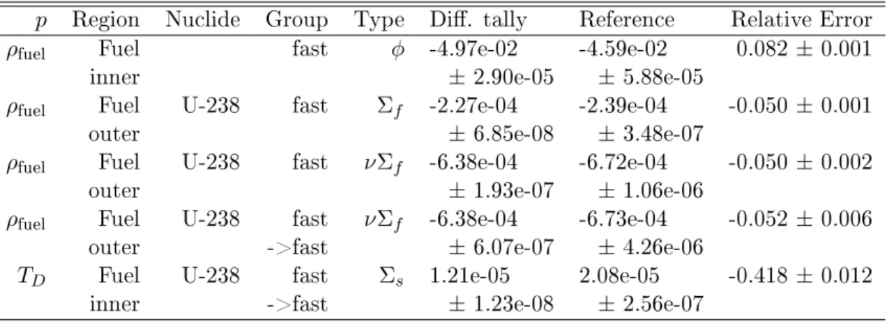
Of the 571 tallies, 328 have acceptably small variance. Of those 328, 323 have relative errors below 0.05. The remaining tallies—derivatives with a large and statistically significant error—are shown in Table 4.3.
The last entry in Table 4.3 shows a clear error in one type of temperature derivative. A typo in the source code has been identified for analog-estimated nuclide-specific tempera-ture derivatives in perturbed materials, but the verification calculations have not yet been repeated. This error is rather specific, and it highlights the importance of a large test suite
with many diverse tallies.
The remaining errors in Table 4.3 are probably due to the 1 𝑆0
𝜕𝑆0
𝜕𝑝 ≈ 0 approximation.
The middle three quantities in the table are 238U fission derivatives in the unperturbed
region of fuel. Because this is an unperturbed region, the contribution derivative is zero,
1 𝑐
𝜕𝑐
𝜕𝑝 = 0, and only the flux derivative is relevant, 𝑋 = ∫︀∫︀∫︀ 𝑐𝜓 1 𝜓
𝜕𝜓
𝜕𝑝. Furthermore, the 238U
fission cross section is only significant at very high energies where neutrons have undergone few collisions. These high energy neutrons have not accumulated many 1
𝑇 𝜕𝑇 𝜕𝑝 or 1 𝐶 𝜕𝐶 𝜕𝑝 terms so the 1 𝑆0 𝜕𝑆0
𝜕𝑝 term presumably has a larger effect. One implication of this discovery is that
the 1 𝑆0
𝜕𝑆0
𝜕𝑝 ≈ 0 approximation might cause poor predictions in fast reactors.
To see more verification results, refer to Tables A.1, A.2, A.3, and A.4 in the appendix. Those tables show a representative sample of the dataset with 264 tallies.
Table 4.3: Tallies from the verification test with large and significant errors. The first column indicates the perturbed variable. The next four columns identify the tallied quantity. The next two columns show the derivatives and the ±𝜎 uncertainty computed with differential tallies and brute-force. The final column shows the relative error.
𝑝 Region Nuclide Group Type Diff. tally Reference Relative Error
𝜌fuel Fuel fast 𝜑 -4.97e-02 -4.59e-02 0.082 ± 0.001
inner ±2.90e-05 ±5.88e-05
𝜌fuel Fuel U-238 fast Σ𝑓 -2.27e-04 -2.39e-04 -0.050 ± 0.001
outer ±6.85e-08 ±3.48e-07
𝜌fuel Fuel U-238 fast 𝜈Σ𝑓 -6.38e-04 -6.72e-04 -0.050 ± 0.002
outer ±1.93e-07 ±1.06e-06
𝜌fuel Fuel U-238 fast 𝜈Σ𝑓 -6.38e-04 -6.73e-04 -0.052 ± 0.006
outer ->fast ±6.07e-07 ±4.26e-06
𝑇𝐷 Fuel U-238 fast Σ𝑠 1.21e-05 2.08e-05 -0.418 ± 0.012
4.2 Improved fitting methods
Differential tallies can potentially be used to improve fitted data models by fitting the derivatives in addition to the zero-order data. This section presents an example application of this technique: fitting the 𝑘eff of a PWR pincell as a function of moderator density.
The same base geometry and material properties from verification problem are used here. The moderator density is varied between 0.6 and 1.0 g / cm3. A reference solution
is calculated by running a simulation with 100 million active neutrons at 10 equally spaced density points. This reference solution is plotted in Figure 4-2.
This discussion will use the weighted linear least squares approach to fitting. Given a set of 𝑛 density points, [𝜌1, . . . , 𝜌𝑛], eigenvalues, [𝑘1, . . . , 𝑘𝑛], and their uncertainties,
Figure 4-2: PWR pincell 𝑘eff as a function of moderator density. Errorbars are omitted
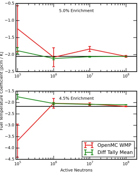
![Figure 1-1: Example of a perturbation calculation using MCNP’s adjoint weighting feature, from [8]](https://thumb-eu.123doks.com/thumbv2/123doknet/14194372.478756/15.918.192.729.593.965/figure-example-perturbation-calculation-using-adjoint-weighting-feature.webp)


![Figure 4-4: The fuel temperature coefficient calculated with OpenMC using three different levels of approximation, compared with results from [16].](https://thumb-eu.123doks.com/thumbv2/123doknet/14194372.478756/52.918.197.683.527.1011/figure-temperature-coefficient-calculated-openmc-different-approximation-compared.webp)