Discovering physics and design trends from visual temporal structures

Discovering Physics and Design Trends from Visual Temporal

Structures

by Donglai Wei

B.S., Mathematics, Brown University, 2011

S.M., Electrical Engineering and Computer Science, M.I.T., 2013

Submitted to the Department of Electrical Engineering and Computer Science in partial fulfillment of the requirements for the degree of

Doctor of Philosophy

in Electrical Engineering and Computer Science at the Massachusetts Institute of Technology

September 2017

Signature of Autho

Certified by:

@

____Signature redacted

Department of ElectricaYEngineering and Computer Science August 31, 2017

Signature redacted,

William T. Freeman Thomas and Gerd Perkins Professor of Electrical Engineering and Computer Science Thesis Supervisor

ccepted by:

Signature redacted

I I ~/ \~'

Leslie A. Kolodziejski Professor of Electrical Engineering and Computer Science Chair, Department Committee on Graduate Students A MASSACHUSETTS INSTITUTE

QF

OCT

2

6 2017

LIBRARIES

ARCHIVES

Discovering Physics and Design Trends from Visual Temporal Structures

by Donglai Wei

Submitted to the Department of Electrical Engineering and Computer Science in partial fulfillment of the requirements for the degree of

Doctor of Philosophy

Abstract

Living in a constantly changing world, we cannot help but notice the temporal regulari-ties of visual changes around us. These changes can be irreversible governed by physical laws, such as glass bottles broken into pieces, or influenced by design trends, such as web pages adopting templates with larger background images. In this dissertation, we build computational models to discover and apply the knowledge of the physics for arrow of time, and the design trends for web pages from image sequences.

In the first part of the thesis, I train models to learn the visual cues that are indicative of the arrow of time from large real world video datasets. In the second part of the thesis, I investigate the evolution of visual cues and layout in web page design through screenshots over time. The knowledge of these visual temporal structures are not only of scientific interest by themselves, but also of practical uses demonstrated in this thesis.

Thesis Supervisor: William T. Freeman

Title: Thomas and Gerd Perkins Professor of Electrical Engineering and Computer Science, M.I.T.

Acknowledgments

I'd first like to thank my thesis advisor, Prof. William T. Freeman. From problem for-mulation to presentation skills, Bill has been a great mentor to guide me throughout my graduate school experience with patience and wisdom. Especially, I deeply appreciate Bill's superb taste in research problems, which pushes me to think more critically and creatively. Beyond teaching me the disciplines of doing research, Bill shows me through his example how to be a researcher with humility, integrity and generosity.

My deep gratitude also goes to my other thesis committee members, Prof. Andrew Zisserman and Prof. Justin Solomon. Andrew has always been a source of great ideas and encouragement during the two projects we collaborated on. Despite his exceptional achievement in the computer vision community, Andrew's passion and detail-oriented attitude towards research teaches me to enjoy the process of pursuing truth. It has always been a fun experience to discuss research questions with Justin, who is quick to decipher the mathematical structure behind the problem and draw connections with other seemingly unrelated topics. Also, I'm thankful to Justin for giving me many insightful and thorough comments on my thesis.

I want to thank other professors and researchers with whom I worked together during my graduate school: Dr. John W. Fisher III, Prof. Fredo Durand, Dr. Ce Liu, Prof. Antonio Torralba, Prof. Bernhard Sch6lkopf, Prof. Changshui Zhang, Prof. Joseph Lim, Prof. Dahua Lin, Dr. Lindsay Pickup, Dr. Zheng Pan, Dr. Yichang Shih, Dr. Jason Chang, Dr. Ali Jahanian, Dr. Phillip Isola, Dr. Neal Wadhwa, Dr. Tali Dekel, Dr. Mikhail Bessmeltsev, Bolei Zhou, and Aric Bartle.

I'm thankful to share an office with Hyun Sung Chang, Roger Grosse, Daniel Zo-ran, Dilip Krishnan, Phillip Isola, Joseph Lim, Neal Wadhwa, Andrew Owens, Tianfan Xue, Jiajun Wu, Zhoutong Zhang and Xiuming Zhang. I will never forget the happy

6

memories and the intensive discussions.

Thank you to my academic advisor Prof. Charles Leiserson, who persuaded me to keep taking courses every year to explore new directions and shared with me his wisdom on academic growth and development. I am also thankful to my other lab-mates and friends in vision and graphics at CSAIL: Biliana Kaneva, Miki Rubinstein, Katie Bouman, Abe Davis, Ronnachai Jaroensri, Michael Gharbi, Guha Balakrishnan, Sebastian Claici and Yu Wang.

Lastly, this thesis is impossible without my parents love and support. Thank you, for everything.

Contents

2 Physics from Temporal Structure: Visual Arrow of Time 23 2.1 Seeing the Arrow of Time . . . . 25

2.1.1 Related Work . . . . 26

2.1.2 D ataset . . . . 26

2.1.3 M odel . . . . 29

2.1.4 Experimental results . . . . 36

2.1.5 D iscussion . . . . 41

2.2 Learning the Arrow of Time . . . . 41

2.2.1 Related Work . . . . 43

2.2.2 ConvNet Architecture . . . . 43

2.2.3 Learning from Simulation Videos . . . . 45

2.2.4 Avoiding Artificial Cues from Real World Videos . . . . 47

8 CONTENTS 2.2.5 Learning from Real World Videos . . . . 2.2.6 Applications . . . . 2.2.7 Discussion . . . . 2.3 Conclusion . . . . 3 Trends from Temporal Structure: Visual Evolution of Web Design

3.1 Related Work ... ... 3.2 WebTrend2l Database . . . . 3.2.1 Database Construction . . . . 3.2.2 Database Pruning . . . . 3.2.3 Database Statistics . . . . 3.2.4 Benchmark Construction . . . . 3.3 Method Overview . . . . 3.4 Trend Visualization for Design Inspiration . . . . 3.4.1 Data and Model . . . . 3.4.2 Analysis . . . . 3.4.3 Application . . . . 3.5 Trend Colorization for Design Prototyping . . . . 3.5.1 Data and Model . . . . 3.5.2 Analysis . . . . 3.5.3 Application . . . . 3.6 Trend Classification for Design Evaluation . . . . 3.6.1 Data and Model . . . . 3.6.2 Analysis . . . . 3.6.3 Application . . . . 3.7 Conclusions . . . . 4 Conclusion Bibliography 53 56 64 64 65 66 67 67 68 73 74 75 76 76 78 81 85 86 86 88 89 89 90 93 94 97 99 8 CONTENTS

List of Figures

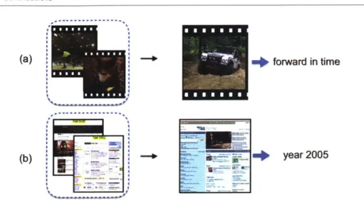
1.1 Discoveries from visual changes. This thesis aim to answer the following two questions: (a) Physics: what visual cues indicate its arrow of time? (Chapter 2) (b) Trends: what makes a 2005 web page look like 2005? (C hapter 3) . . . . 21 2.1 Arrow of Time Challenge: given five frames from each video, can you tell

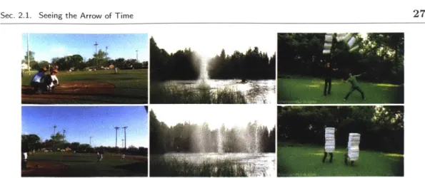
if the frames are ordered in the forward direction of time or the reversed? (answer key belowl) . . . . 24 2.2 Three examples of videos from our TA180 YouTube dataset, including

one reverse-time example (right-most frames). The sampled frames are shown following the video frame order from top to bottom. . . . . 27 2.3 Overview of the motion consistency (MC) method. We show three frames

from a sequence in the TennisBall13 dataset, where a ball is rolled into a stack of static balls. Bottom row: regions of motion, identified using only the frames at t and t - 1. Notice that the two rolling balls are identified as separate regions of motion and colored separately in the bottom right-most plot. The fact that one rolling ball (first frame) causes two balls to end up rolling (last frame) is what the motion-consistency method aims to detect and use.. . . .. . . . . 30

2.4 Overview of the auto-regressive (AR) method. Top: tracked points from a se-quence, and an example track. Bottom: Forward-time (left) and backward-time (right) vertical trajectory components, and the corresponding model residuals. Trajectories should be independent from model residuals (noise) in the forward-time direction only. For the example track shown, p-values for the forward and backward directions are 0.5237 and 0.0159 respectively, indicating that forward

tim e is m ore likely. . . . . 32

2.5 Overview of the bag-of-words (BoW) method. Top: pair of frames at

times t - 1 and t +1, warped into the coordinate frame of the intervening

image. Left: vertical component of optical flow between this pair of frames; lower copy shows the same with the small SIFT-like descriptor grids overlaid. Right: expanded view of the SIFT-like descriptors shown left. Not shown: horizontal components of optical flow which are also

required in constructing the descriptors. . . . . 34

2.6 Left: construction of the divergence operator by summing contributions along

straight-edge segments of a square superimposed on the flow word grid. Center

& right: positive and negative elements of the div operator, respectively. . . . 36

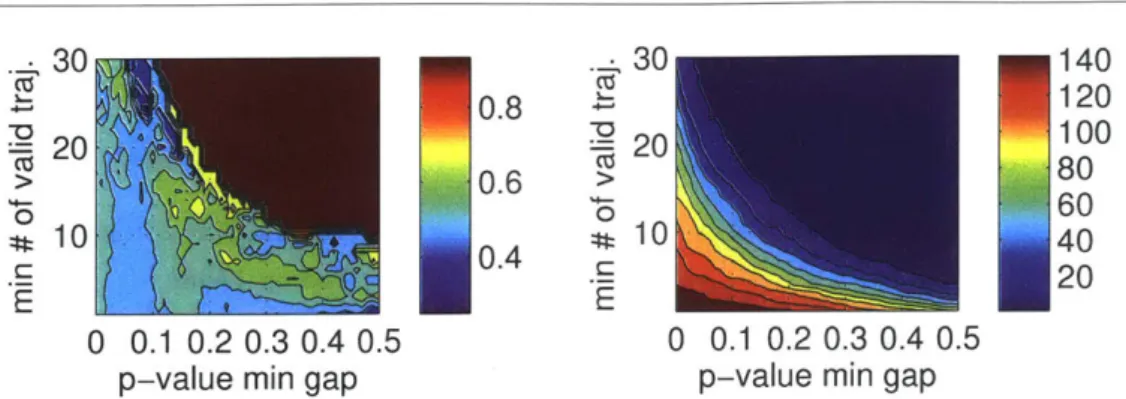
2.7 Left: Accuracy of AR model classifications over the 2D parameter space. Right:

number of videos accepted. The AR model is particularly effective for small numbers of videos; as we force it to classify more, the performance falls to near

chance level. . . . . 38

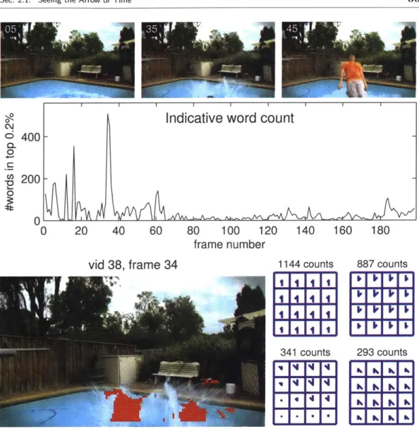
2.8 Video from the test set, correctly classified as being backwards in time. The

most informative point in the video is the few frames around 34 (shown), where there is an inverse splash of water. Red dots here mark the locations of all strongly-backwards flow words. This type of motion (shown in the four flow

word grids) was learned to be strongly indicative of a backwards time direction. 39

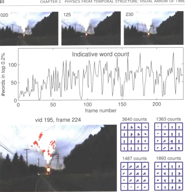
2.9 Video from the test set, correctly classified as being forwards in time. The most

informative forwards-time words refer to the motion of the billowing steam, and occur periodically as the steam train puffs. Red dots marked on frame 224 show

the locations of the most-forwards 10 flow words in this frame. . . . . 40

LIST OF FIGURES

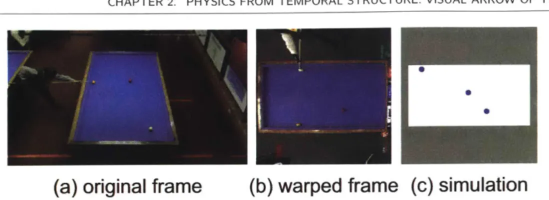
2.10 Illustration of the temporal class activation map network (T-CAM) for arrow of time (AoT) classification. Compared to the traditional VGG architecture for image recognition, (b) we first concatenate the conv5 features from the shared convolutional layers, (c) and then replace the fully-connected layer with convolution layers and global average pooling layer (GAP) [37,57,58,73] for better localization. . . . . 44 2.11 The 3-cushion billiard dataset. (a) Original frame from a 3-cushion video;

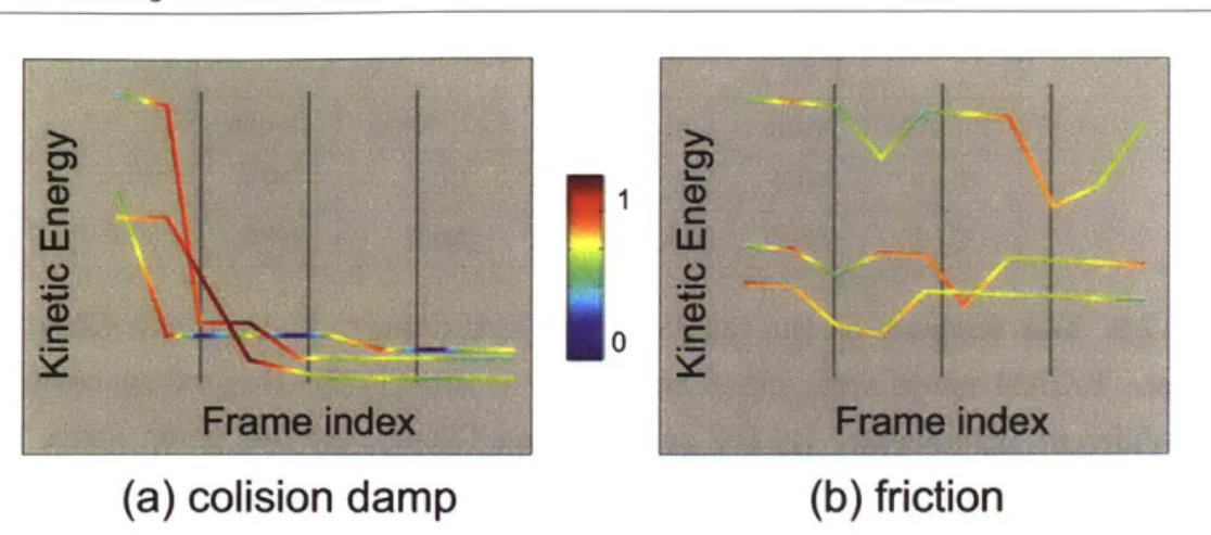
(b) the frame warped (with a homography transformation) to an over-head view of the billiard table; and, (c) a simulated frame to match the real one in terms of size and number of balls. . . . . 46 2.12 Visualization of test accuracy for sampled billiard ball videos. (a) For

the system with only collision damping as the arrow of time signal, the model learns to detect the time of sudden drop of energy and becomes unconfident otherwise; (b) For the friction signal, however, the model is barely confident most of the time due to the weak signal. . . . . 47 2.13 Illustration of artificial signals from videos in UCF101 dataset. (a) The

black framing of the clip has small non-zero intensity value, and a vertical slice over time displays asymmetric temporal pattern. (b) After training on the UCF101 test data, there are clusters corresponding to camera zoom -in. . . . . 48 2.14 The MJPEG Arrow of Time dataset. It consists of around 16.9k videos

without inter-frame video coding from Vimeo. The dataset mostly con-tains human actions, and the rest are of various contents (e.g. water, anim als, vehicle). . . . . 50

2.15 Heatmaps of correct predictions from the Flickr-AoT dataset. We use the "jet colomap" to indicate the probability of being forward (red, close to 1) or backward (blue, close to 0) and we only overlay the region where T-CAM is confident. We compute the flow for two consecutive frames in the middle of the clip. The black arrows indicate the direction and the magnitude (normalized by the largest value) of the flow on the sparse grid, and they are only shown for the colored regions. Our network learns to focus on the regions that inform about the AoT in both (a) general and (b) human scenes. (a) The network utlizes basic physics (e.g., water falling due to gravity) and video biases (e.g., people film trains coming towards them more often than trains leaving from them) to correctly decide the AoT. (b) When there is a human in the scene, the network decides the AoT by observing human actions. . . . . 55 2.16 Browser interface for our Amazon Mechanical Turk study to obtain

hu-man perforhu-mance on the arrow of time prediction. . . . . 56 2.17 Heatmap results on the Hollywood-AoT dataset. (a) In these successful

cases, our model utilizes basic physics (i.e., gravity) and human expres-sions to correctly decide the AoT, whereas (b) in some cases, the model fails to discriminate that the video is played backwards. Although the model fails overall in the train sequence, it extracts the correct AoT from the train steam . . . . . 59 2.19 Common cues for reverse film detection (cont. next page). For each

reversely-played clip, we show its first, middle and last frame and its heatmap (blue for backward and red for forward) with normalized flow vector on the middle frame. Ideally, the heatmap should be blue, indi-cating the clip is played in the backward direction . . . . 60 2.19 The T-CAM model consistently focuses on regions with (a) head motion,

(b) motion against gravity, and (c) human body motion. The blue regions indicate that (a) global head motion and eye movement and (b) upward motion patterns of water and snow can be correctly recognized by the T-CAM model for backward AoT. For (c), the T-CAM model can be fooled by professional backward-acting (second row) and subtle motion (third row) where red regions are around performers. . . . . 61

2.20 Test accuracy on the lip reading dataset. (a) input motion of mouth region and (b) distribution of test accuracy over different words. ... . 63 3.1 Tag cloud visualization of top-100 web domains in our WebTrend2l

database. The size of the web domain name is in proportion to the number of web page screenshots. . . . .

68

3.2 Examples of bad web pages to prune. We remove web pages with ren-dering errors, either happened at the server-side during (a) capture and (b) retrieval, or at the browser-side during (c) loading. To remove web pages with disqualified content, we filter out (d) web pages that are no longer functional. . . . . 69 3.3 Histogram of the mean intensity of our web page dataset. We find that (a)

the histogram has several sporadic peaks, (b) especially in the intensity range between 200 and 255. In the main text and Figure 3.4, we identify the cause of each of the four groups of peaks. After pruning, (c) the histogram varies smoothly with the mean intensity value. . . . . 69 3.4 Examples of web pages identified through mean intensity histogram method.

(a) white pages, (b) google pages, (c) browser-side error, (d) server-side error. . . . . ... . . .. . . . . 70 3.5 Examples of web pages identified through geometry-based method. (a)

pages that are under construction tend to have big page margins, and (b) pages that are rendered without proper CSS files tend to have big page height. . . . . 71 3.6 Examples of web pages identified from their html source code. (a) If

the html source code does not have any body text, errors like "page not found" or "unfinished loading" can happen. Two common errors can be found through matching the keyword of (b) "Index of' and (c) "sorry." 72 3.7 Distribution of data over years and distribution of colors over years.

Magnitudes are in a logarithmic scale. The color space is a discretized

version of sRGB with 4 bins per channel, and sorted based on hue. . . . 73

13

3.8 Benchmark preprocessing. In height, we crop out the top 729 pixels for the first impression, avoiding over-compressing (a) long scrolled-down pages. In width, we crop out (b) one-sided margin due to the html layout not adapting to the browser window width and keep (c) two-sided m argin by design. . . . . 74 3.9 Variational autoencoder model. Given input images, the model learns to

compress them into more compact representation with the encoder mod-ule, which can well recover the original input with the decoder module. We only use the encoded mean vector p for our latent code. . . . . 76 3.10 Comparison of VAE trained with different dimensions of latent variable.

(a) we plot the reconstruction error over epoch number (the error does not go to zero partly due to the noise injected in the sampling module to avoid overfitting); (b) we show qualitative comparisons for three sampled images; (c) covariance matrix of 20 axes of latent representations with largest variance. With #z > 100, the learned representation becomes distributed, not concentrating on certain dimensions. . . . . 77 3.11 Variational autoencoder model. Given input images, the model learns

to compress them into more compact representation with the encoder module, which can well recover the original input with the decoder module. 78 3.12 Visualization for the first ten eigenvectors. For the first two year groups,

blue and yellow are main colors. . . . . 80 3.13 Visualization for the first ten eigenvectors. For the first two year groups,

blue and yellow are main colors. . . . . 81 3.14 2D representation from t-SNE. We first bin the t-SNE code into 40x40

grid cells and average over images whose codes belong to each cell. This 2D map is purely based on the appearance of web pages without any year labels, where each region correspond to one trend of design. Later, with year labels, we visualize how the design trends change over time. 82 3.15 For each year, we show the heatmap of the ratio of images at each rounded

grid position. . . . . 83

3.16 Visualization of the nonlinear manifold learned by VAE. (a) We use t-SNE to project the latent code onto the 2D plane and round up the posi-tion to regular grid point; (b) for each group year, we show the heatmap of the ratio of images at each rounded grid position. The heatmaps change continuously over time, showing the design trend shift. For example, late 1990s web pages often have white margins or colorful background color, while 2010s web pages mostly have wide images at the top of the page. 84 3.17 Top 20 most frequent colors in each year. Magnitudes are in logarithmic

scale. The color space is a discretized version of sRGB with 4 bins per channel, sorted based on hue. Through this analysis, we observe that the Internet is getting duller (less saturated) and a wider, more evenly spread, range of colors is being used as time progresses (distribution over colors is becoming higher entropy). . . . . 85 3.18 Conditional Generative Adversarial Network model. Given input gray

scale images, the generator model outputs a color image, and the dis-criminator model classify if the input-output pair is fake or real. . . .. 85 3.19 Qualitative results for web page re-colorization by models trained on

different groups of years. (a-d) input web pages are from 1996-2000, 2001-2005, 2006-2010, 2011-2016 respectively. . . . . 87 3.20 Illustration of the bricolage colorization application. Given (b) manually

stitched web pages from (a) input templates, pix2pix models trained on web pages from different periods generate (c) diversified and self-consistent colorization from the gray-scale image of (b). . . . . 88 3.21 Illustration of our convolutional neural network, VGG-CAM [73]. Given

an input web page, the model predicts its year label. The first five groups of convolutional layers (blue) are the same as VGG-16. Then there are three 1 x 1 convolutional layers (yellow) to replace the fully-connected layers in VGG-16. In the end, after a global-average-pooling layer (orange) and a softmax layer, we obtain the probability of the year label for the input web page. . . . . 90

15

3.22 Test results for VGG-CAM model. (a) confusion matrix for the ex-act year classification, (b) confusion matrix for the prediction to be within one year range of the ground truth, (c) example web pages from "brown.edu", where the design trend can last for several years which makes it hard to predict the exact year of a web page. . . . . 91 3.23 Here we show, for each predicted year, the top four web pages our model

is most confident belong to that year, revealing designs that are highly characteristic for each year, such as simple textual web pages in the 1990s, and more image-heavy designs of the 2010s. . . . . 92 3.24 Visualization of VGG-CAM neurons at different layers. We show all

64 filters for conv1 units and four sample filters for conv3 and pool5. Noticeably, the VGG-CAM learns mostly horizontal and vertical edges (conv1), simple shapes (conv3), and more complex visual patterns like logos and faces (pool5). . . . . 94 3.25 Heatmap of predicted years for web pages. We show (a) four input web

pages ranging from 1996 to 2016 and (b) the predicted 14x 14 heatmap of predicted years, scaled to the image size. Our model learns to find the logo region in the example from 1996 and the text region in the example from 2016 out of date. . . . . 95 3.26 These two web pages might seem generic, but each reflects the design

trend of its own era. Can you tell what makes the 2016 web page look like 2016? Over each example web page above, we show regions our algorithm thinks are diagnostic of that web page's year. On each row, one patch from the web page is shown, followed by four patches, from other pages, that the algorithm considers to have a similar visual pattern. Noticeably, the old design (1996) mainly uses simple text and textual links for communicating the content, and a modern design (2016) applies more diverse graphical elements such as special fonts for text, graphic logos, and natural images. . . . . 96

List of Tables

2.1 Arrow of time classification results on the TennisBall13 and TA180 dataset. (a) the accuracy on TennisBall13 is high due to its small number of videos (b) we compare all four methods with 3-fold cross-validation on TA180: spatial-temporal orientated energy (SoE), motion consistency (MC), auto-regressive (AR), bag-of-words (BoW) . . . ..37 2.2 Test accuracy on the simulated 3-billiard datasets and the real video. We

compare T-CAM model with either one (T=1) or two (T=2) temporal segments for three different experiments. (1) For no signal case (None), the test performance is at the chance level; (2) Both models perform well when there is only collision damping in the system (Col.), but temporal fusion on conv5 helps to learn weak signals like friction (Fric.). (3) the simulation Col.+Fric. is made with a similar system configuration to the real videos (3-cush.), where the collision damping signal dominates. Thus, both models have similar performance. . . . . 48 2.3 An examination of the artificial cues for arrow of time prediction. We

show results of controlled experiments on the effect of black framing and camera motion on UCF1Ol. . . . . 51 2.4 Effect of temporal codec on MJPEG-AoT dataset. We train and test

on three versions of the MJPEG-AoT dataset and our model has similar performance. Thus, the added codec signal doesn't introduce significant artificial signals for our model to capture for the arrow of time. .... 52

2.5 Test accuracy of the T-CAM model trained on the Flickr-AoT train dataset. (a) we first compare different parameters of the T-CAM model on the Flickr-AoT test dataset.(b) Other datasets: the MJPEG-AoT and the TA180 of [43]. T-CAM (raw) is trained on a larger set of videos from Flickr without pre-processing. . . . . 54 2.6 Feature learning results for action recognition on UCF-101 split-1. We

list out important factors besides the network initialization methods: input, architecture and layers to fine-tune. For the flow input, our ini-tialization from arrow of time prediction is consistently better than the previous state-of-the-art ImageNet initialization [65] when only the fc layers are fine-tuned. . . . . 58 3.1 Colorization errors on different groups of years. We test four models

trained on different years of web pages and a model trained on all years. We compute the L2 distance between the ground truth ab color channel and that from output. The model trained on each year group performs the best when tested on the same year group. . . . . 88 3.2 Test accuracy for year label prediction on WebTrend2lColorization errors

on different groups of years. To show that the . . . . 91

Chapter 1

Introduction

"No man ever steps in the same river twice, for it's not the same river and he's not the same man."

Heraclitus, "Heraclitus : 139 Fragments" trans. John Burnet

W

different levels. For atoms in

iso-lated physical systems, the Second Law of Thermodynamics dictates their uni-directional change to reach higher levels of randomness. Not to mention design trends which are born and died equally fast.

Growing up in this dynamic environment, we unconsciously learn about statistical regularities from these diverse visual changes. For example, we will be more surprised if we see water drops to come together than to splatter, as it is against our statistical

knowledge of how things should change. Given a web page, we can often tell if its

design looks out of fashion by finding statistical commonalities with web pages we visited before. Can we build computers to have the similar intelligence to discover these temporal structures?

Beyond scientific understanding, the knowledge of temporal statistical structures can have a wide range of applications. For example, in video forensics, i.e. identifying if a video is manipulated, such temporal knowledge can tell if some frames have been deleted or added to fake a persons presence in a surveillance video. In web page design, understanding the trend of each era can help designers to come up with layout and color schemes that are either in fashion or out of date and give feedback on which part of the web page looks outdated.

However, compared to the extensive work on statistical structures for single im-ages [7, 16, 29, 45, 52], there has been far less investigation for temporal structures for image sequences [17]. Recently, the temporal ordering of image sequences, a specific statistical property of temporal structures, is learned to reorder a collection of images

CHAPTER 1. INTRODUCTION

from different cameras chronologically [5, 10] and to learn useful visual features for other vision tasks [14, 15, 41, 46] , e.g. action recognition. In this promising direction, we not only need deeper scientific understanding of the temporal structures, e.g. what visual cues do the models capture, but also new statistical properties of temporal structures with broader applications.

In this thesis, we investigate two different statistical properties of temporal struc-tures: direction and trend (Figure 1.1). We work on image sequences from different research communities: real world videos in computer vision, and web designs in the hu-man computation interfaces. By exploiting the statistical structure of visual changes, we develop novel applications which can be used for video forensics and give interactive feedback during different stages of web page design process. Below, we give a high-level overview of my thesis, along with contributions and other works done during my doctoral program.

* 1.1 Overview

First, we address the question: "what visual cues are indicative of the arrow of time, i.e. the one-way direction of changes?" We train convolutional neural networks (CNN) to classify whether input videos are playing in the forward or backward direction. A

model that can perform this task well can be used for video forensics and abnormal event detection, and its learned features are useful for other tasks, such as action recognition. However, CNNs can "cheat" and learn artificial signals from video production instead of the real signal. We design controlled experiments to systematically identify superfluous signals. After controlling these confounding factors, we analyze the visual cues learned on the large-scale Flickr video dataset, revealing both semantic and non-semantic cues for arrow of time and the photographer bias during video capture.

Next, we answer the question: "what makes 2016 web pages look like designed in 2016?" We first collect a large-scale dataset containing screenshots for top 11,000 popular web domains over 21 years (1996-2016). Trained on this database, our models investigate the design trend through visualization, colorization and evaluation. For visu-alization, we train variational autoencoder models to learn interpretable representations for design exploration on a 2D plane intuitively. For colorization, we use conditional generative adversarial networks to learn to re-colorize input web pages with different 20

Sec. 1.2. Contributions

(a)

Figure 1.1: Discoveries from visual changes. This thesis aim to answer the following two questions: (a) Physics: what visual cues indicate its arrow of time? (Chapter 2)

(b) Trends: what makes a 2005 web page look like 2005? (Chapter 3)

color palettes based on their content and year labels. Finally, we train a CNN to predict the years in which input web pages were created and identify visual elements that are ahead of or lagging behind the trend.

* 1.2 Contributions

In this thesis, we expand the frontier of statistical understanding of temporal structures in the following three ways:

1. Building large-scale databases. To extract reliable and generalizable statistics for temporal structures, we need a massive amount of image sequence data. We collect two real world video databases for the arrow of time work and a database for web design screenshots over 21 years, all publicly available for the community. 2. Analyzing learned representations. Besides the competitive performance of the learned representations, we use methods to interpret the learned by the algo-rithm.

3. Exploring new applications. We propose novel applications to exploit the obtained knowledge of temporal statistical structures.

CHAPTER 1. INTRODUCTION * 1.3 My Other Work

In this thesis, motion is used as input to shed light on videos' statistical temporal struc-tures, revealing high-level knowledge of physics, trend and style. During my doctoral program, I also studied motion perception from four different perspectives: estimation, representation, segmentation and visualization.

Under the supervision of Dr. Ce Liu and Prof. William T. Freeman, I applied the data-driven matching framework, commonly used for high-level vision problems like semantic parsing, to improve the traditionally physics-based motion estimation in stereo and flow [69]. With Prof. Dahua Lin and Dr. John W. Fisher III, I studied the manifold of object deformations with Lie algebra representation and parallel transport technique [68]. With Dr. Jason Chang and Dr. John W. Fisher III, I co-developed a video motion segmentation method based on Dirichlet process models with Gaussian random field models on top [8]. I also participated in deviation magnification [63] with Dr. Neal Wadhwa, Dr. Tali Dekel and Prof. William T. Freeman. Interested readers can refer to these publications for details.

Chapter 2

Physics from Temporal Structure:

Visual Arrow of Time

"Let us draw an arrow arbitrarily. If as we follow the arrow we find more and more of the random element in the state of the world, then the arrow is pointing towards the future; if the random element decreases the arrow points towards the past.

That is the only distinction known to physics."

- Arthur Eddington, The Nature of the Physical World

H

be time-reversed without us noticing that something is amiss (Figure 2.1)? At a small scale, the physics of the world is reversible. Most fundamental equations look the same in both forward and backward directions of time. The collision of two particles looks the same if time is reversed. Yet at a macroscopic scale, time is not reversible and the world behaves differently whether time is playing forwards or backwards. For example, for a cow eating grass or a dog shaking water from its coat, we do not automatically accept that a complicated system (chewed food or the spatter pattern of water drops) will re-compose into a simpler one.

This seemingly innocent question is deeply-connected with fundamental properties of time. In physics, such asymmetric nature of temporal structures in our world is called the "arrow of time" (AoT), which has been studied in the context of thermodynamics and cosmology [44,47]. While physics addresses whether the world is the same forwards and backwards, our goal is to assess whether and how the direction of time manifests itself visually. Can we train a machine to make that same judgment? What is it that lets us see that time is going the wrong way in reversed videos?

Apart from the fundamental science, the arrow of time plays important roles in

CHAPTER 2. PHYSICS FROM TEMPORAL STRUCTURE: VISUAL ARROW OF TIME

Figure 2.1: Arrow of Time Challenge: given five frames from each video, can you tell if the frames are ordered in the forward direction of time or the reversed? (answer key belowl)

different areas of artificial intelligence. First, the arrow of time is a natural supervision signal for videos, i.e. we can trivially obtain supervision labels (i.e. the direction in OForwards: (a), (c), (e); backwards: (b), (d). Though in (c) the motion is too small to be visible to the eye.

Sec. 2.1. Seeing the Arrow of Time

which the video is played) for massive amount of data to train large-scale classifiers. Besides the prediction task, these arrow of time labels can be used to learn visual representations for other video classification tasks, e.g. action recognition [15,41]. Second, and more generally, temporal asymmetry priors have implications for methods for video processing, e.g. video decompression, optical flow estimation, and photo-sequencing [5]. Also, causal inference, of which the arrow of time is a special case, has been connected to machine learning topics, such as transfer learning and covariate shift adaptation [51].

In this chapter, we address the following questions for the direction of visual changes: 1. Can computers learn from human knowledge of physics to see the arrow of time

in videos?

2. Can computers instead learn by themselves simply through watching real world videos? Further, what visual cues will they learn to use?

* 2.1 Seeing the Arrow of Time

Through our daily experience, we have unconsciously learned to "see" the arrow of time in videos, i.e. we can perceive if videos are playing in the forward or backward direction. In this section, we address the question: How can we teach computers?

Specifically, we formulate our approach within the framework of video classification, where we train classifiers to predict the direction in which the input video is played, i.e. forward or backward. For each video, we want to know not only how strong is its signal indicating the arrow of time, but also in which regions can we predict it reliably. We seek to use low-level visual information - closer to the underlying physics - to see the arrow of time, not object-level visual cues. We are not interested in learning that cars tend to drive forward, but rather in studying the common temporal structure of videos. We expect that such regularities will make the problem amenable to a learning-based approach. Some videos will be difficult or impossible; others may be straightforward.

In the sequel, we first curate two video datasets as common test beds for the arrow of time classification in Section 2.1.2. Then in Section 2.1.3, we propose four different ways to incorporate our knowledge of physics into machine learning algorithms to classify the direction of videos. We compare and analyze classification results of our models above in Section 2.1.4.

CHAPTER 2. PHYSICS FROM TEMPORAL STRUCTURE: VISUAL ARROW OF TIME

* 2.1.1 Related Work

Learning and representing statistical structures of visual input are crucial for a variety of computer vision tasks. These structures can capture both the spatial properties of images and temporal properties of image sequences.

For the spatial structure, many algorithms [16] are developed to exploit different aspects of the spatial regularity. For example, the now widely-used multi-resolution spatial pyramid architectures and convolutional neural networks[7, 34] are evolved from the statistical question, "Are images invariant over scale?" Many more statistical ques-tions are asked to learn properties of human visual processing: "Can we recognize faces upside down?" [52], or about tonescale processing by asking, "Can we recognize faces if the tonescale is inverted?" [29]. Especially, to our interest, both symmetry and asym-metry properties of spatial structures are useful for visual inference. The assumption that light comes from above is asymmetric and helps us disambiguate convex and con-cave shapes [45]. Spatial translation invariance, on the other hand, allows us to train object detection or recognition systems without requiring training data at all possible spatial locations.

For the temporal structure [17], there has been far less investigation. Several recent papers have used temporal ordering. Basha et al. [5, 10] consider the task of photo-sequencing - determining the temporal order of a collection of images from different cameras. Others have used the temporal ordering of frames as a supervisory signal: for learning an embedding in [46]; for self-supervision training of a ConvNet [15, 41]; and to construct a representation for action recognition [14]. We here focus on a simple property of the temporal structure, i.e. temporal direction, asking: "Are video temporal statistics symmetric in time?"

* 2.1.2 Dataset

We collect two video datasets for the arrow of time classification task. The first Ten-nisBall13 dataset, consisted of videos shot by ourselves with simple content, serves as a controlled environment to illustrate our new algorithms. The second TA180 dataset, containing general videos downloaded from Youtube, represents the complex visual world.

___________________ -j

Sec. 2.1. Seeing the Arrow of Time 27

Figure 2.2: Three examples of videos from our TA180 YouTube dataset, including one reverse-time example (right-most frames). The sampled frames are shown following the video frame order from top to bottom.

TennisBaII13 dataset We film a small number of video clips using a camera with the Motion-JPEG codec [49], which compresses each frame independently without artifacts holding any time-direction information. This dataset comprises 13 HD videos of tennis balls being rolled along a floor and colliding with other rolling or static balls. An example of one of these sequences is used later in Figure 2.3.

EVALUATION PROCEDURE. Tests on the TennisBall13 dataset are run in a leave-one-out manner, because of the small size of the dataset. Specifically, classification models will be trained on 12 videos (and their various flips), and then tested on the withheld video, and all 13 possible arrangements are run.

YouTube dataset (TA180) This dataset consists of 180 video clips from YouTube, which are obtained manually using more than 50 keywords. Our goal is to retrieve a diverse set of videos from which we might learn low-level motion-type cues that indicate the direction of time. Keywords include "dance," "steam train," and "demolition," among

other terms. The dataset is available at http: //www. robots. ox. ac. uk/data/arrow/.

SELECTION CRITERIA. Video clips are selected to be 6-10 seconds long, giving at

least 100 frames on which to run computations. Thus, we discard clips from many professionally-produced videos where each shot's duration is too short, since each clip is required to be a single shot. We restrict the selections to HD videos, allowing us to subsample extensively to avoid block artifacts and minimize interactions with any given

CHAPTER 2. PHYSICS FROM TEMPORAL STRUCTURE: VISUAL ARROW OF TIME

compression method.

Videos with poor focus or lighting are discarded, as are videos with excessive camera motion or motion blur due to hand shake. Videos with special effects and computer-generated graphics are avoided, since the underlying physics describing these may not match exactly with the real-world physics underpinning our exploration of the arrow of time. Similarly, split-screen views, cartoons and computer games are all discarded. Also, videos are required to be in landscape format and minimal interlacing artifacts. In a few cases, the dataset still contains frames in which small amounts of text or television channel badges have been overlaid, though we try to minimize this effect as well.

Intentionally, the dataset contains clips from "backwards" videos on YouTube; these are videos where the authors or uploaders have performed the time-flip before submit-ting the video to YouTube, so any time-related artifacts that might have been introduced by YouTube's subsequent compression will also be reversed in these cases relative to the forward portions of our data. In these cases, because relatively few clips meeting all of our criteria exist, multiple shots of different scenes are taken from the same source video in a few cases. In all other cases, only one short clip from each YouTube video is used.

In total, there are 180 videos in the dataset and 25 of them are reversed intentionally by youtube uploaders to achieve special effects. Two frames from each of three example videos are shown from top to bottom in Figure 2.2. The first two are forwards-time examples (baseball game, water spray), and the right-most pair of frames is from a backwards-time example where pillows are "un-thrown." During learning, we feed the algorithms both the original video and their reversed versions, to avoid the unbalanced label distribution of the downloaded videos.

EVALUATION PROCEDURE. For evaluating the methods described below, the dataset is divided into 60 testing videos and 120 training videos, in three different ways such that each video appeared as a testing video exactly once and training exactly twice. For parameter selection, the 120 videos of the training set are further sub-divided into 70 training and 50 validation videos. The three train/test splits are labeled A, B and C, and are the same for each of the methods we report. The backwards-to-forwards video ratios for the three test sets are 9:51, 8:52 and 8:52 respectively.

The evaluation measure for each method is the proportion of the testing videos on 28

Sec. 2.1. Seeing the Arrow of Time 29

which it could correctly predict the time direction.

U 2.1.3 Model

There are many underlying physical reasons why the forward and reverse time directions may look different on average. Below we probe how the arrow of time can be determined from video sequences in four distinct ways, drawing intuitions from energy, entropy, causality and statistical patterns.

Energy-based: Spatio-temporal oriented energy (SoE) In classical mechanics, the kine-matic energy of a system changes in certain patterns. The energy may decrease in time due to its dissipation, and may fluctuate while in equilibrium. We use the "Spatio-temporal oriented energy" (SOE) [11] as an off-the-shelf method to describe how the kinematic energy changes from the video motion.

SOE is a filter-based feature for video classification, which is sensitive to differ-ent space-time textures. Our implemdiffer-entation is faithful to that laid out in [11], and comprises third-derivative-of-Gaussian filters in eight uniformly-distributed spatial di-rections, with three different temporal scales. As in the prior work, we split each video into 2 x 2 spatial sub-regions, and concatenate the SOE responses for each sub-region for form a final feature.

Entropy-based: motion consistency (MC) Stated by the second law of thermodynamics, the total entropy of an isolate system can only increase. Thus, it is far more common for one motion to evolve into multiple motions than for multiple motions to collapse into one consistent motion. For instance, the cue ball during a snooker break-off hits the pack of red balls and scatters them, but in a reverse-time direction, it is statistically highly unlikely that the initial conditions of the red balls (position, velocity, spin etc.) can be set up exactly right, so that they come together, stop perfectly, and shoot the cue ball back towards the cue.

To exploit this observation of motion consistency, we first find pixels in the video where frame intensity differences are above a threshold. Then, we grow these pixels into consistent regions and compare them with those in the previous frame. These regions are illustrated in Figure 2.3. Broadly speaking, we expect more occurrences of one region splitting in two than of two regions joining to become one, in the forwards-time direction.

30 CHAPTER 2. PHYSICS FROM TEMPORAL STRUCTURE: VISUAL ARROW OF TIME

frame 104 frame 114 m e 3-3

Figure 2.3: Overview of the motion consistency (MC) method. We show three frames from a sequence in the TennisBall13 dataset, where a ball is rolled into a stack of static balls. Bottom row: regions of motion, identified using only the frames at t and t - 1. Notice that the two rolling balls are identified as separate regions of motion and colored separately in the bottom right-most plot. The fact that one rolling ball (first frame) causes two balls to end up rolling (last frame) is what the motion-consistency method aims to detect and use.

IMPLEMENTATION DETAILS. Given the image at current time t (It), we warp the next

frame (It+,) to it with estimated homography, which yields a warped image Wt+1.

The difference bewteen the current frames and the warped frame, I(It - Wt+1) , now

highlights moving areas. A smooth-edged binary mask of image motion is made by summing this difference over color channels, resizing down to 400 pixels, convolving with a disk function and then thresholding. The different regions in the motion mask are enumerated. Where one or more regions at time t intersect more than one region

each at time t - 1, a violation is counted for that frame pair, since this implies motion

merging. We count the violations for each time direction of a sequence separately, with a variety of parameter settings. We use three different threshold-radius pairs: radii of 5, 6.6 and 8.7 pixels, and corresponding thresholds of 0.1, 0.01 and 0.056, where image intensities lie between 0 and 1. Finally, we train a standard linear SVM using the violation counts as 6d features (two time-directions; three parameterizations).

Causality-based: auto-regressive (AR) Researchers have recently studied the question of measuring the direction of time as a special case of the problem of inferring causal direction in cause-effect models. Peters et al. [42] shows that, for non-Gaussian additive noise and dynamics obeying a linear ARMA (auto-regressive moving average) model, the noise added at some point of time is independent of the past values of the time series, but not of the future values. This allows us to determine the direction of time by independence testing, and Peters et al. [42] uses it to successfully analyze the direction of time for EEG data. Intuitively, this insight formalizes our intuition that changes (noise) added to a process at some point of time influences the future, but not the past. Here we consider the AR model, a special case of ARMA without the moving average part. However, we deal with vector-valued time series, which strictly speaking goes beyond the validity of the theoretical analysis of Peters et al. [42]. We find that a second order AR model works well in our setting. In a nutshell, we model the time series' next value as a linear function of the past two values plus additive independent noise.

The assumption that some image motions will be modeled as AR models with additive non-Gaussian noise leads to a simple algorithm for measuring the direction of time in a video: track the velocities of moving points, fit those velocities with an AR. model and perform an independence test between the velocities and model residuals

(errors). This process is illustrated in Figure 2.4.

The independence testing follows the work of [42], and is based on an estimate of the Hilbert-Schmidt norm of the cross-covariance operator between two reproducing kernel Hilbert spaces associated with the two variables whose independence we are testing. The norm provides us with a test statistic, and this in turn allows us to estimate a p-value for the null hypothesis of independence. If the p-value is small, the observed value of the norm is very unlikely under the null hypothesis and the latter should be rejected. Ideally, we would hope that the p-value should be small (i.e. close to 0) in the backward direction, and large (i.e. significantly bigger than 0) in the forward direction.

IMPLEMENTATION DETAILS. We analyze the motion of a set of feature points extracted

by KLT trackers [39,60], running tracking in both forward and backward directions.

For each tracked point, velocities are extracted, and a 2D AR model is fitted. We then test the independence between the noise and velocity to determine the arrow of time

31 Sec. 2.1. Seeing the Arrow of Time

32 CHAPTER 2. PHYSICS FROM TEMPORAL STRUCTURE: VISUAL ARROW OF TIME 0.5 1 - backward velocity -- backward noise 0 0.5 -0.5 0 forward velocity -foward noise -1 -0.5 0 50 100 150 200 0 50 100 150 200 Frame Frame

Figure 2.4: Overview of the auto-regressive (AR) method. Top: tracked points from a se-quence, and an example track. Bottom: Forward-time (left) and backward-time (right) vertical trajectory components, and the corresponding model residuals. Trajectories should be indepen-dent from model residuals (noise) in the forward-time direction only. For the example track shown, p-values for the forward and backward directions are 0.5237 and 0.0159 respectively, indicating that forward time is more likely.

at the trajectory level.

Inferring causal direction of AR. process is only possible when the noise is non-Gaussian, and when noise in only one temporal direction is independent. We define a valid trajectory to be one which spans at least 50 frames, for which noise in at least one direction is non-Gaussian as determined by a normality test, and for which the p-value test in one time-direction gives p < 0.05 whereas in the other it gives p > 0.05 + 6 for some minimal gap 6 (i.e. exactly one direction fails the null hypothesis test).

All valid trajectories are classified as forward or backward according to their p-value scores. Ideally, all valid trajectories for one video should imply the same direction of time, but in practice, tracking can be noisy in a way that violates the time-series model assumption. For this, we reject the videos with fewer than N valid trajectories, where

N > 1. We classify the accepted videos by a majority vote among the valid trajectories. We thus get a binary classifier (with the possibility of rejection) at video level. While

hypothesis testing is used to classify single trajectories, the overall procedure is not a hypothesis test, and thus issues of multiple testing do not arise. The hypothesis testing based trajectory classifiers can be seen as weak classifiers for video and the voting makes a strong classifier.

Statistics-based: Bag-of-Word (BoW) In the above three methods, we manually design the visual features from videos to capture known physical quantities, i.e. energy, entropy and causality. Besides physics, statistics-based perceptual priors are also indicative of the arrow of time. For example, it is physically possible for a man to walk backward while facing front, but we may think it more natural for the reverse which has higher probability to happen in our daily experience. Here we design visual features to capture such statistical regularity of the input. Inspired by the "bag-of-words" method for object recognition [36], we apply it to our optical flow input to discover motion clusters, referred to as flow words, exhibiting temporal asymmetries.

Each flow word is based on a SIFT-like descriptor of motion occurring in small patches of a video. We first register the frames of a video in order to compensate for hand-shake and intentional camera motion (panning and zooming etc.), and then we assume that any residual motion is due to objects moving in the scene. Rather than computing a SIFT based on image edge gradients, motion gradients from an optical flow computation are substituted, giving a descriptor which represents local histograms of image motion. An example of the descriptors used to build these flow words is shown

in Figure 2.5.

These object-motion descriptors are then quantized to form a discrete set of flow words, and a bag-of-words descriptor representing the entire video sequence is thus computed. With sufficient forward and reverse-time examples, a classifier can be trained to discriminate between the two classes.

IMPLEMENTATION DETAILS. In a similar manner to [64], computation starts from dense trajectories. However, instead of only representing the histogram of optical flow over a region, as in the HOF features of [33], we also represent its spatial layout in a local patch in a manner similar to a local SIFT descriptor.

In detail, frames are downsized to 983 pixels wide in a bid to remove block-level artifacts and to provide a consistent image size for the rest of the pipeline. Images at time t - 1 and t + 1 are registered to the image at time t, and an optical flow

33 Sec. 2.1. Seeing the Arrow of Time

CHAPTER 2. PHYSICS FROM TEMPORAL STRUCTURE: VISUAL ARROW OF TIME N1 '1 '4 'N 'I I I '7 /

Figure 2.5: Overview of the bag-of-words (BoW) method. Top: pair of frames at times t - 1 and t

+1

computation is carried out [6]. This is repeated over the video sequence in a temporal sliding window, i.e. giving T - 2 optical flow outputs for a sequence of length T. These outputs take the form of motion images in the horizontal and vertical directions. A normal VLFeat dense SIFT descriptor [61] uses intensity gradient images in the x-and y-directions internally in its computations, so to describe the flow maps instead of

iI

Sec. 2.1. Seeing the Arrow of Time 35 the image structure, we simply operate on the vertical and horizontal motion images instead of the intensity gradients. This yields motion-patch descriptors whose elements represented the magnitudes of motion in various directions passing through the tth frame, on a small 4 x 4 grid (bin size 6 pixels) sampled once every 3 pixels in the horizontal and vertical directions.

We suppress static trajectories, because we are only interested in dynamic behaviour for this work. This is achieved by setting the motion-gradient images to zero where the magnitude is below a threshold, and not including motion-patch descriptors from such areas in further processing. This excises large areas, as can be seen in the constant background color in Figure 2.5.

DIVERGENCE OPERATOR FOR FLOW WORDS:. In analyzing the results, it will be useful

to quantify the divergence or other motion-field properties of a given flow word descrip-tor. Using the divergence theorem, we make an approximation to the integral of the divergence over a descriptor by considering the net outward and inward motion fluxes across a square that joins the centers of the four corner cells on the descriptor grid, assuming that motion at every point within a grid cell is drawn independently from the histogram which is represented at the centre of that cell. The resulting divergence operator for flow words is shown in the central and right parts of figure 2.6, with the negative and positive flux contributions separated for visualization.

LEARNING. _{A dictionary of 4000 words is learnt from a random subset of the training} data (O(10) examples) using K-means clustering, and each descriptor is assigned to its closest word. A video sequence is then described by a normalized histogram of visual flow words across the entire time-span of the video. Empirically, performance is improved if the square roots of the descriptor values are taken prior to clustering, rather than the raw values themselves.

For each video in the training/validation set, we extracted four descriptor his-tograms: (A): the native direction of the video; (B): this video mirrored in the left-right direction; (C): the original video time-flipped; and (D): the time-flipped left-right-mirrored version. An SVM is trained using four histograms A-D extracted from each video of a training set, 280 (4 x 70) videos in total. Similarly, the 50 videos of the validation set generate 200 histograms A-D in total, and each is classified with

36 CHAPTER 2. PHYSICS FROM TEMPORAL STRUCTURE: VISUAL ARROW OF TIME

Construction Pos Div Neg Div

*4

1

Figure 2.6: Left: construction of the divergence operator by summing contributions along straight-edge segments of a square superimposed on the flow word grid. Center & right: positive

and negative elements of the div operator, respectively.

the trained SVM. For a valid classification, A and B must have one sign, and C and

D another. We combine the SVM scores as A

+

positive score for forwards clips, a negative score for backwards clips, and some chance to self-correct if not all of the component scores are correct.

The C parameter for the SVM is chosen to be the value that maximizes the classi-fication accuracy on the validation set over all three train/test splits. Once this C pa-rameter is fixed, the whole set of 120 training videos, including the previously-withheld validation set, is used to learn a final SVM for each train/test split.

Testing proceeds in a similar manner to that used for the validation set: the SVM scores for the four bag-of-words representations for each testing video are combined as

A

+

N 2.1.4 Experimental results

We first show how well our models can predict the arrow of time on two video datasets. Then, for the bag-of-words model, we visualize its confident prediction regions and the motion clusters that the model learns to use.

Classification accuracy On the TennisBall13 dataset, we only train and test motion consistency method and bag-of-words method. Due to the strong arrow of time signal in the dataset, both methods predict correctly 12 out of 13 times. Note that the

7/

/

F

/T\

/T\