Magnetic storm-induced enhancement in neutral composition at low latitudes as inferred by O(¹D) dayglow measurements from Chile

HAL Id: hal-00317645

https://hal.archives-ouvertes.fr/hal-00317645

Submitted on 23 Sep 2004

HAL is a multi-disciplinary open access

archive for the deposit and dissemination of

sci-entific research documents, whether they are

pub-lished or not. The documents may come from

teaching and research institutions in France or

abroad, or from public or private research centers.

L’archive ouverte pluridisciplinaire HAL, est

destinée au dépôt et à la diffusion de documents

scientifiques de niveau recherche, publiés ou non,

émanant des établissements d’enseignement et de

recherche français ou étrangers, des laboratoires

publics ou privés.

composition at low latitudes as inferred by O(1D)

dayglow measurements from Chile

D. Pallamraju, S. Chakrabarti, C. E. Valladares

To cite this version:

D. Pallamraju, S. Chakrabarti, C. E. Valladares. Magnetic storm-induced enhancement in neutral

composition at low latitudes as inferred by O(1D) dayglow measurements from Chile. Annales

Geo-physicae, European Geosciences Union, 2004, 22 (9), pp.3241-3250. �hal-00317645�

Annales Geophysicae (2004) 22: 3241–3250 SRef-ID: 1432-0576/ag/2004-22-3241 © European Geosciences Union 2004

Annales

Geophysicae

Magnetic storm-induced enhancement in neutral composition at low

latitudes as inferred by O(

1

D) dayglow measurements from Chile

D. Pallamraju1, S. Chakrabarti1, and C. E. Valladares2

1_{Center for Space Physics, Boston University, 725 Commonwealth Avenue, Boston, MA, 02215, USA} 2_{Boston College, Institute of Space Research, 140 Commonwealth Avenue, Chestnut Hill, MA, 02467, USA}

Received: 3 October 2003 – Revised: 3 March 2004 – Accepted: 8 March 2004 – Published: 23 September 2004 Part of Special Issue “Equatorial and low latitude aeronomy”

Abstract. We describe the effect of the 6 November 2001

magnetic storm on the low latitude thermospheric composi-tion. Daytime red line (OI 630.0 nm) emissions from Car-men Alto, Chile showed anomalous 2–3 times larger emis-sions in the morning (05:30–08:30 Local Time; LT) on the disturbed day compared to the quiet days. We interpret these emission enhancements to be caused due to the increase in neutral densities over low latitudes, as a direct effect of the geomagnetic storm. As an aftereffect of the geomagnetic storm, the dayglow emissions on the following day show gravity wave features that gradually increase in periodicities from around 30 min in the morning to around 100 min by the evening. The integrated dayglow emissions on quiet days show day-to-day variabilities in spatial structures in terms of their movement away from the magnetic equator in response to the Equatorial Ionization Anomaly (EIA) development in the daytime. The EIA signatures in the daytime OI 630.0 nm column-integrated dayglow emission brightness show differ-ent behavior on days with and without the post-sunset Equa-torial Spread F (ESF) occurrence.

Key words. Atmospheric composition and structure

(Air-glow and aurora; Thermosphere-composition and chemistry; Instruments and techniques)

1 Introduction

The Earth’s upper atmosphere receives different inputs of en-ergy from the Sun at different latitudes. During magnetically quiet periods the high latitudes receive most of the energy from particle precipitation, which is nearly equal in magni-tude with that of the solar extreme ultraviolet (EUV)

radia-Correspondence to: D. Pallamraju

(dpraju@bu.edu)

tion over the equatorial and low latitudes. However, during geomagnetic disturbances the particle energy inputs over the high latitudes can be larger by a factor of more than an order of magnitude (Mayr et al., 1978). Mayr et al. (1978) pro-posed a circulation mechanism by which the neutrals from the high latitudes are transported to the lower latitudes during storm time. Intense Joule heating takes place over the high latitudes during geomagnetic storms which causes both hor-izontal and vertical winds, that redistributes the neutral den-sities. This heating also causes an upwelling of the neutral species over the auroral oval, which generates a large wave that is capable of propagating to the magnetic equator in a few hours (Mayr et al., 1978; Prolss, 1993). There are ample evidences of an increase in the neutral temperature and winds at low latitudes during magnetic storms (Mayr and Volland, 1973; Meriwether et al., 1973; Mayr et al., 1978; Prolss, 1980; Burrage et al., 1992; Prolss, 1993; Burns et al., 1995; Fuller-Rowell et al., 1996; Pant and Sridharan, 1998; Fuji-wara et al., 1996; Emmert et al., 2001). The thermospheric winds and composition changes are intimately coupled and as a consequence, the F-region electron densities also change accordingly. These changes in the temperature and dynam-ics affect changes in the composition at all latitudes. Satellite data have indicated that the densities of all species increase at low latitudes during geomagnetic storms (Hedin et al., 1977; Mayr et al., 1978). Simulation results show that the Trav-eling Atmospheric Dynamics (TADs) launched in northern and southern polar regions during magnetic storms propa-gate towards low latitudes at high speeds (about 670 ms−1at 260 km), causing thermospheric density increase at low lat-itudes due to compression and compressional heating of the thermospheric gas (Fujiwara et al., 1996). Wind Imaging In-terferometer (WINDII) on board the Upper Atmospheric Re-search Satellite (UARS) measured winds of around 650 ms−1 at 200 km for a storm whose Kp value was 7.7 (Zhang and

0 12 24 12 24 12 24 0 2 4 6 8 10 Kp Index 19:20 7:20 19:20Local Time (Hrs.)7:20 19:20 7:20 19:20 Kp Ap

5 November 2001 6 November 2001 7 November 2001

0 75 150 225 300 Ap Index 0 12 24 12 24 12 24 Universal Time (Hrs.) -300 -200 -100 0 100 DST Index (nT) 19:20 7:20 19:20 7:20 19:20 7:20 19:20

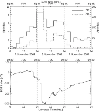
Fig. 1. (Top): Kp and Apindices for three days 5–7 November

2001. The scales for Kpand Ap are shown on the left and right

axes, respectively. Kp index shows a value of more than 4

dur-ing the late afternoon hours on 5 November. 6 November is a dis-turbed day with both Kp and Ap indices of 9− and 300

respec-tively. The magnetic disturbance effect is not seen over low lat-itudes on 5 and and 7 November, as can be seen by the low Ap

indices on these days. (Bottom): Dst variation for the three days

under study is shown. The vertical dashed line in both the panels show the 00:00 UT time for the 6 and 7 November data. Storm sudden commencement occurred on the early hours of 6 November and the Dst reached a value of −300 nT, indicating a severe storm

occurrence. Local time is indicated in the topside of the plot.

Shepherd, 2000). As discussed above, such winds are known to redistribute the molecular rich gas brought up due to up-welling at high latitudes.

In this study, we report on the daytime OI 630.0 nm red line airglow emission enhancements generated by the geomagnetic-storm-induced changes in composition over low latitudes. The daytime measurements were carried out with the High-Resolution Imaging Spectrograph, using an Echelle grating (HIRISE) instrument (Pallamraju et al., 2002) from Carmen Alto in Chile. Unusual emission en-hancements were obtained in the morning hours when the equatorial electrodynamics is not expected to show appre-ciable variations. Simultaneous GPS-derived Total Electron Content (TEC) measurements do not show any TEC increase, clearly implying no role of electron densities in the observed emission enhancement. Using this information and with the understanding of the storm time behavior of the low-latitude upper atmosphere, we interpret that the neutral density en-hancements are responsible for the observed dayglow emis-sion enhancements. Our measurements also show wave

pe-riodicities of 45 to 90 min in the dayglow emissions. In particular, the day following the geomagnetic storm shows wave periodicities increasing from 30 min in the morning to 100 min by the evening, most probably indicating the after-effects of the magnetic storm on the neutral dynamics (i.e. winds and tides). Moreover, the latitudinal variations in the dayglow emissions on quiet days show different features in terms of the EIA development. The day with a stronger EIA development, seen as early as around 14:00 LT, in the day-glow emissions is followed by the post-sunset ESF onset.

2 Instrumentation

Optical measurements of the airglow emissions are an impor-tant means to understanding upper atmospheric phenomena. While ground-based nighttime optical airglow measurements at various wavelengths have been carried out for several decades, systematic daytime optical airglow measurements have started only recently (see review by Chakrabarti, 1998). The main challenge for the daytime optical measurements is the strong solar background continuum, which is approxi-mately three orders of magnitude brighter than the daytime airglow emissions. At Boston University we have developed a high-resolution (0.12 ˚A at 630.0 nm) imaging echelle spec-trograph called the HIRISE (Pallamraju et al., 2002), which has been used to understand the Ring effect variation in the sky spectrum as opposed to the Fraunhofer spectrum (Pal-lamraju et al., 2000), observations of the sunlit auroral arcs (Pallamraju et al., 2001), and the daytime magnetospheric cusps (Pallamraju et al., 2004) in the OI 630.0 nm emissions. It is necessary to take the Ring effect (filling in of Fraun-hofer lines by the scattering due to molecules in the Earth’s atmosphere) into account while making spectrographic day-glow measurements. The details on the Ring effect variation and the procedure employed for the data reduction to obtain the daytime emissions using HIRISE have been described in detail elsewhere (Pallamraju et al., 2000; 2002). In this study we discuss the behavior of observed emission rates on dif-ferent days, both with and without geomagnetic storm occur-rence.

3 Data description and analysis

We present a case study of the effect of the 6 November 2001 geomagnetic storm on the OI 630.0 nm dayglow emis-sions. Clear sky conditions prevailed for a stretch of 10 days centered on the day of the magnetic storm at Car-men Alto (23.16◦S, 70.66◦W; 10.6◦magnetic latitude), Chile, from where the HIRISE was operated. For the present inves-tigation, we present data from 5–7 November 2001.

Figure 1 shows the Kp, Ap and Dst variations for three

days 5–7 November 2001. Kpindex indicates that the high

latitude disturbance effects started during the second half of 5 November. By the beginning of 6 November, the Kpindex

and Dst value showed sudden changes from around 4 to 9−

D. Pallamraju et al.: Magnetic storm-induced enhancement in neutral composition 3243 was a disturbed day with severe disturbances of Kp=9−for

six hours and Kp=7 for another three hours in the beginning

of the day (corresponding to a Dst of around −300 nT for

4–5 h and an Ap index of 300 for six hours). 7 November

shows a gradual recovery with Kp=2. The Apindex, which

most closely describes the effect of magnetic disturbances at low and equatorial latitudes, shows only 6 November to be a severely disturbed day with a peak index of 300 (compared to 5 and 7 November with peak Ap around 50). The daily

average values, <Ap>, for the three days were 21, 142 and

19, respectively. The solar F10.7 cm fluxes for the three days were similar (230.6, 230.2, and 263.9, respectively).

To appreciate the behavior of the red line dayglow emissions during storm time, one needs to understand its excitation mechanisms. The upper state of the red line is O (1D), which is a metastable state with an associated energy of 1.96 eV, and has a lifetime of around 110 s. The red line emission is a doublet with transitions at 630.0 and 636.4 nm having a branching ratio of 3:1. The production mechanisms for this emission are (see reviews by Hays et al., 1978; Solomon and Abreu, 1989):

– (P1) Photoelectron Impact: O(3P) + e∗−(−−−−−−E>1.96 eV)→O(1D) + e – (P2) Photo-Dissociation: O2+hν λ=(135−175 nm) −−−−−−−−−→(1D) + O(3P) and, – (P3) Dissociative Recombination: O+₂ +e −→O(1D) + O(3P) .

Loss of this excited state occurs through one of the following two processes: – (L1) Loss of O(1D) by Quenching: O(1D) + (N2,O2,O(3P), e) −→O(3P) + (N2,O2, (3P), e) and, – (L2) Loss of O(1D) by Radiation: O(1D) −→O(3P) + hν(λ=630.0 and 636.4 nm) where, O (3P) is the ground state.

The top panel of Fig. 2 shows the zenith OI 630.0 nm red line emissions for 5 November 2001, along with the

±1σ measurement error. Five minutes of data have been coadded to reduce the statistical uncertainties – the maxi-mum uncertainty is around ±15% at noontime. The x and y axes, respectively, represent the local time and the emission brightness in Rayleighs (R). It can be seen that the emission

6 8 10 12 14 16 18 Local Time (Hrs.) 0 1000 2000 3000 4000 5000

OI 630.0nm Emiss. Rate (Rayleighs)

5 November 2001 <Ap> = 21 I_(Total): Measured I_(SZA) : Estimated 6 8 10 12 14 16 18 Local Time (Hrs.) -1000 0 1000 2000 3000

Dynamical component of Dayglow

I_(Total) - I_(SZA)

Fig. 2. (Top): Zenith column-integrated OI 630.0 nm dayglow emission rate from Carmen Alto (solid line) and the solar zenith angle (dotted) contribution for 5 November 2001 are depicted along with ±1σ error bars. The x and y axes represent the local time and the column-integrated emission rate in Rayleighs. The SZA depen-dent dayglow contribution is obtained by assuming a (cosine)0.5 behavior for this variation with SZA and normalizing it with the measured dayglow emissions at around 07:30 LT. The value of the averaged Ap index for the day is shown on top left. (Bottom):

Difference between the total column-integrated dayglow emissions and SZA component of the dayglow. This represents the dynamical component in the optical emissions. The negative values represent the “trough-like” features of the wave features. Attention should be paid mainly to the amplitudes of the wave features and not to the negative or positive values alone. A monotonic increase is seen towards afternoon, which is a response of the EIA development.

rates range from 1000 R in the morning to around 4000 R at around 15:00 LT, followed by a gradual decrease towards the evening. These values are in good agreement with the WINDII data, which measured 3500 R during noon for sim-ilar solar flux and at simsim-ilar latitude (S. Zhang, 2003, pri-vate communication). In addition to the broad diurnal vari-ability described above, one can also notice smaller scale-size (1–2 h) variabilities in the dayglow emissions. From the list of the production mechanisms, it can be noted that the mechanisms P 1 and P 2 vary as a function of the solar zenith angle (SZA) as both photoelectrons and solar photons (in S-R continuum), vary depending on the position of the

6 8 10 12 14 16 18 Local Time (Hrs.) 0 1000 2000 3000 4000 5000

OI 630.0nm Emiss. Rate (Rayleighs)

6 November 2001 <Ap> = 142 I_(Total): Measured I_(SZA) : Estimated 6 8 10 12 14 16 18 Local Time (Hrs.) -1000 0 1000 2000 3000

Dynamical component of Dayglow

I_(Total) - I_(SZA)

Fig. 3. Same as in Fig. 2 but for 6 November 2001. Notice the rise in emissions in the morning above the dotted line (SZA vari-ation), which is approximately equal to the typical afternoon peak emissions and a factor of 2–3 increase when compared with the morning quiet time emissions (see Fig. 5). The SZA variation used for this day is the same as the one used for all three days. The increase in emissions in the dynamical component in the morning 05:30–08:30 LT (bottom panel) is 4–5 times larger than the typical dynamical variations on a quiet day (see Fig. 5). This brightening is interpreted to be due to the changes in neutral composition over low latitudes. These changes are brought about by neutral winds from high latitudes and TAD triggered by the magnetic storm.

Sun. Hence, these two mechanisms are not expected to show the small-scale variations seen in the emissions. Therefore, it follows that the Dissociative Recombination process (P 3) is most likely responsible for such observed variations. The variation in the electron density can give rise to the observed variabilities, as it is known that, in addition to the produc-tion of electrons due to the solar photons, several dynamical effects, such as equatorial electrodynamics, traveling iono-spheric disturbances (TIDs), etc., give rise to significant vari-ations in the local electron densities (Kelley, 1989; Sastri, 2002; Sastri et al., 2002). Also, variabilities in the column-integrated emissions can be brought about by changes in the neutral composition due to the transport from the high lati-tudes, propagation of the gravity waves, neutral winds, etc. (Fujiwara et al., 1996; Balthazor and Moffet, 1997).

6 8 10 12 14 16 18 Local Time (Hrs.) 0 1000 2000 3000 4000 5000

OI 630.0nm Emiss. Rate (Rayleighs)

7 November 2001 <Ap> = 19 I_(Total): Measured I_(SZA) : Estimated 6 8 10 12 14 16 18 Local Time (Hrs.) -1000 0 1000 2000 3000

Dynamical component of Dayglow

I_(Total) - I_(SZA)

Fig. 4. Same as in Fig. 2 but for 7 November 2001. Notice the peri-odicities of small-amplitude oscillations, which seem to increase in time periods from around 30 min in the morning to around 100 min in the evening. Whether such a behavior in wave activity is an af-tereffect of severe magnetic storms is currently under investigation, as such an increase in the wave periodicities are not seen on the two previous days.

To understand the variabilities that are not caused by the SZA variation, they have to be isolated from the total emissions. A (cosine(SZA))0.5 behavior is assumed for the SZA induced O (1D) production. Considering the measured morning dayglow emissions as initial estimates, we fit such cosine-type variation for the dayglow for the rest of the day. In the low and equatorial latitudes, the daytime electrody-namical variation is an important feature that shows signifi-cant day-to-day variability. This equatorial electrodynamics generates a plasma fountain over the equator that develops as the equatorial ionization anomaly (EIA) in the low latitudes by afternoon (see reviews by Moffet, 1979 and Raghavarao et al., 1988a). The column-integrated dayglow emissions also show the signature of the development of the EIA. However, the morning dayglow emissions are not expected to be af-fected by such large-scale equatorial electrodynamical varia-tion. With that assumption, we fit the measured dayglow with a SZA varying dayglow behavior by normalizing it with the total dayglow emissions at around 07:30 LT. The SZA vari-ation obtained by normalizing at 07:30 LT for 7 November

D. Pallamraju et al.: Magnetic storm-induced enhancement in neutral composition 3245 is employed for all the three days (shown as the dotted line

in the top panel). As the days are consecutive no significant change in the SZA behavior is expected between each of the days. The bottom panel of Fig. 2 shows the difference be-tween measurements on 5 November and the SZA varying contribution (IT OT–ISZA), which now represents brightness

variation, both due to electrodynamical and dynamical (i.e. TADs or gravity waves) effects in the low-latitude upper at-mosphere. As this figure displays dynamical behavior of the upper atmosphere, the negative values represent the “trough-like” features of the waves. Earlier studies have shown that the EIA crest development starts at around 09:00 LT (Mof-fet, 1979; Raghavarao et al., 1988a; Walker et al., 1994; Yeh et al., 2001). Normalizing at any time earlier than around 09:00 LT would result in similar variations as represented by IT OT–ISZAabove, with varying negative and positive

magni-tudes due to the wave features. However, as we are interested in the amplitude of oscillations alone, the choice of the exact time (before 09:00 LT) for normalization is not very critical. Attention should be paid mainly to the amplitude of the wave features and not to the negative or positive values only.

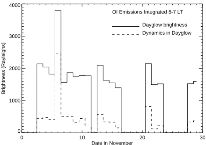
Figures 3 and 4 show similar analysis for the disturbed day (6 November) and another quiet day (7 November 2001), re-spectively. The maximum measurement uncertainty on both these days is about ±12%. The disturbed day, too, shows smaller-scale wave-like features similar to those on the quiet days. Compared to the 5 November data, one can notice that 6 November brightness shows a sharp increase in the morn-ing hours between 05:30–08:30 LT (top panel) with peak val-ues around 4000 R. In fact, as it can be noticed that the emis-sions at this time are the highest for the whole day, which is not a typical quiet day behavior (see top panels of Figs. 2, 4 and Fig. 5). Figure 5 shows the averaged dayglow emissions in the morning hours (06:00–07:00 LT) centered around the emission enhancements seen on 6 November. The x axis of this figure shows the day of the month and the y axis is the brightness in Rayleighs. The solid line shows that the day-glow emissions on 6 November are a factor of 2–3 larger when compared with other days, while the dynamical com-ponent (dashed line) shows a factor of 4–5 larger contribution on the disturbed day.

7 November 2001 daytime emissions (Fig. 4 top panel) show interesting aspects in the behavior of the wave features, with periodicities increasing during the course of the day. The diurnal trend on this day is similar to that on 5 Novem-ber, although the peak emissions in the afternoon hours are smaller (around 3000 R). Oscillations in the emissions are much larger than the count statistics and they seem to be in-creasing in periodicities from 30 min (morning) to 100 min (evening). Such behavior is not seen on the previous two days. Currently, analysis is underway to investigate if such a behavior is an aftereffect of severe geomagnetic storms simi-lar to the one that occurred on the previous day. As the three days under investigation are consecutive, the same SZA vari-ation is employed for all of them. Similar analysis as ex-plained for the 5 November data is employed for the next two days. The difference between the total integrated

col-0 10 20 30 Date in November 0 1000 2000 3000 4000 Brightness (Rayleighs) OI Emissions Integrated 6-7 LT Dayglow brightness Dynamics in Dayglow

Fig. 5. The average variations of the dayglow brightness (solid line) and the brightness in the dynamical variations (dashed line) dur-ing morndur-ing hours for 17 days in the month of November. Notice a factor of 2–3 and 4–5 enhancements in the dayglow brightness and in the dynamical component on the disturbed day (6 November when compared with the average variations on the quiet days of the month).

umn dayglow emissions and the normalized SZA variation for 6 November is shown in the bottom panel of Fig. 3. One can notice a period (05:30 to 08:30 LT) of enhanced emis-sions with as high as around 3,000 R at around 06:30 LT. To appreciate the spatial extent of the effect of morning rise in the emissions, and the response of the upper atmosphere dur-ing the disturbed day (in comparison to the quiet days), it is useful to investigate the behavior of the dynamical com-ponent over a larger field-of-view. Similarly, the dynamical component on 7 November (bottom panel of Fig. 4) is similar to that on 5 November for this view angle. Again, as we will show below, the behavior over a larger field-of-view displays a different perspective of the spatial variations in emissions on all the days.

As the HIRISE is an imaging spectrograph, light incident from different view directions is recorded on different pixels of the detector. For this campaign, observations were carried out over a 140◦field-of-view. Assuming a constant emission altitude of 230 km (Hays et al., 1978; Solomon and Abreu, 1989; Witasse et al., 1999) for the redline dayglow emis-sions, these view angles can be approximated to different latitudes. They correspond to approximately 7◦ _{in latitude}

from 6.5◦ _{to 13.5}◦ _{magnetic latitude (south). Assuming a}

“uniform” thickness of the emission layer, we corrected the data in different view directions for the van Rhijn effect. We subtracted the assumed SZA variation for each view direc-tion following a similar procedure as described for the zenith measurements. Figures 6–8 shows 2-dimensional plots of the dynamical component in dayglow for 5–7 November, respec-tively. The x axis indicates the local time, the y axis shows the magnetic latitude in the Southern Hemisphere and the color scale represents the dynamical component in relative brightness. It should be remembered that emissions from any

-1000.0 -500.0 0.0 500.0 1000.0 1500.0 2000.0 2500.0 3000.0 Rayleighs

Dynamics in Dayglow (5 Nov 2001)

6 8 10 12 14 16 18 Local Time (in Hrs.)

7 8 9 10 11 12 13

Magnetic latitude (in degrees)

Fig. 6. Two-dimensional plots of the dynamical component in the dayglow for 5 November 2001. The x axis represents the local time and y axis indicates the approximate magnetic latitude in the South-ern Hemisphere from where the emissions are assumed to have orig-inated. A constant emission altitude of 230 km has been assumed to estimate the magnetic latitudes. The color scale indicates the bright-ness variation due to the dynamics of the upper atmosphere in the red line emission region (similar to the bottom panel of Fig. 2). A peak is seen centered at around 13:00 LT at 9◦magnetic latitude, which is most likely the response to the EIA development. This weaker development of the EIA as seen in the dayglow emissions, is an indication of weaker equatorial electrodynamics and hence no post-sunset ESF is expected for this night. Compare this day with the 7 November data (Fig. 8) when a stronger EIA development occurred.

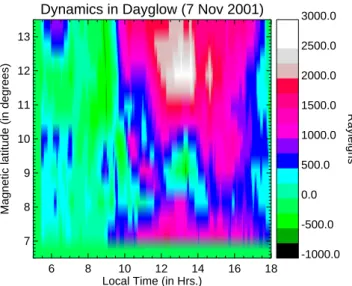
view angle other than for the zenith “cuts across” different latitude locations and as such, the magnetic latitudes (shown on the y axis) should be treated as a representative value only. First, we will discuss the behavior of emissions on the quiet days: 5 and 7 November (Figs. 6 and 8). Data from 5 November do not show any brightness enhancement in the morning in any latitude. However, a peak in the emis-sions is seen during 11:00–15:00 LT at around 9◦magnetic latitude. Such emission peaks in the afternoon are most likely due to the variations in the electron densities, which develop in response to the variations in the equatorial elec-trodynamical drifts and electric fields. Such dayglow emis-sion enhancements can be seen as the optical manifestations of the EIA development in the bottomside F-layer (Pallam Raju et al., 1996). In comparison, the data on 7 November shows a stronger development of the EIA with a peak around 13:00 LT over 11◦–13◦magnetic latitude – farther away from the magnetic equator when compared to 5 November data. Such strong development of the EIA in the daytime is con-ducive for the post-sunset ESF occurrence, and has been sug-gested as a possible precursor to the onset of the post-sunset ESF (Raghavarao et al., 1988b; Sridharan et al., 1994). Such differences in the dayglow emission rates in terms of emis-sion peak occurrence closer to the magnetic equator versus

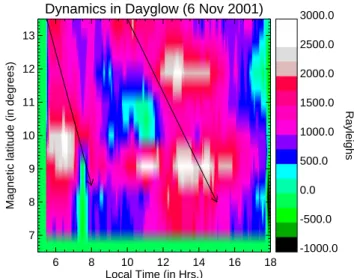
-1000.0 -500.0 0.0 500.0 1000.0 1500.0 2000.0 2500.0 3000.0 Rayleighs

Dynamics in Dayglow (6 Nov 2001)

6 8 10 12 14 16 18 Local Time (in Hrs.)

7 8 9 10 11 12 13

Magnetic latitude (in degrees)

Fig. 7. Same as in Fig. 6 but for 6 November 2001. Notice the sharp rise in the emissions during the morning hours (05:30–08:30 LT), which are 4–5 times larger than the emissions of dynamical com-ponent on quiet days, as can be seen in Figs. 5, 6 and 8. The time duration of morning rise is larger in 9◦–13.5◦magnetic latitudes compared with the duration of increase in 7◦–9◦magnetic latitudes. Emission enhancements are also seen around 12◦and 9◦magnetic latitudes at 12:30 LT and 13:30 LT, respectively, most likely indi-cating propagation of neutral species from high to low latitudes. The arrow indicates a possible direction of the phase propagation of the neutral species from high to low latitudes. The contribution of the dynamical component is largest on this day compared with the quiet days shown in Figs. 6 and 8, possibly due to the presence of comparatively larger neutral densities that are redistributed by the magnetic storm effects.

“emission crest” occurrence farther away from the equator in the afternoon hours on 5 November and 7 November, respec-tively, show examples of typical non-ESF and ESF “days”. Ionograms from digisonde at Jicamarca confirmed the oc-currence of the post-sunset ESF on 7 November as opposed to the 5th. Recently Mendillo et al. (2001) and Valladares et al. (2001) supported the correlation between the sunset time EIA strength with the post-sunset ESF onset. Indeed the TEC measurements on 5 November and 7 November, re-spectively, show poorly developed and well developed EIA crests at 18:00 LT, respectively (Fig. 9), thereby providing an independent confirmation of the conclusions arrived at by the daytime optical measurements around 4 h earlier. The development of the EIA takes place earlier in the lower F-region (the altitude F-region to which OI 630.0 nm dayglow is most sensitive) first before registering an effect on the top-side of F-layer (where TEC measurements are more sensi-tive), possibly explaining the differences in times of obser-vations of the crest development by the dayglow and by the radio measurements. This feature of daytime optical emis-sions could potentially be used to provide an advance warn-ing for the ESF onset. Details of these aspects of the behav-ior of the daytime optical measurements compared with the radio measurements and their relationship to the post-sunset

D. Pallamraju et al.: Magnetic storm-induced enhancement in neutral composition 3247 -1000.0 -500.0 0.0 500.0 1000.0 1500.0 2000.0 2500.0 3000.0 Rayleighs

Dynamics in Dayglow (7 Nov 2001)

6 8 10 12 14 16 18 Local Time (in Hrs.)

7 8 9 10 11 12 13

Magnetic latitude (in degrees)

Fig. 8. Same as in Fig. 6 but for 7 November 2001. Notice the strong emissions at around 12◦−13◦magnetic latitude at 13:00 LT. This represents the optical signature of the development of the EIA in the daytime. This day shows relatively stronger EIA development compared with 5 November (see Fig. 6). Such strong EIA devel-opments are conducive for post-sunset ESF occurrence. Jicamarca digisonde data confirmed the post-sunset ESF occurrence on this night. Enhanced 630.0 nm emissions in the afternoon may prove to be the crucial precursors to the post-sunset ESF occurrence.

ESF development would be described in a future publication. Although the dynamical component in the afternoon on both the quiet days shows differences in terms of the EIA devel-opment (Figs. 6 and 8), the behavior in the morning on both days is similar in that neither day shows any emission en-hancements. The inter-hemispheric asymmetry in the TEC crests on 7 November is most likely due to meridional winds blowing from south to north.

In comparison to the quiet days, the magnetically dis-turbed day, 6 November (Fig. 7), shows emission enhance-ments by a factor of 4–5 in the morning from 05:30–08:30 LT over almost all the latitudes of observation. The temporal ex-tent of the enhancement is larger in the 9◦– 13.5◦magnetic latitude sector as compared to the 7◦–9◦ magnetic latitude sector. The afternoon peak emission at around 13:00 LT is approximately equal to the peak morning emissions. Also, one can notice phase propagation in these relative emissions towards the low latitudes, as indicated by the arrows on the plot. The emission enhancements in the afternoon at around 12:30 LT at 12◦magnetic latitude and at around 13:30 LT at 9◦magnetic latitude are most likely due to such phase prop-agation from the high latitudes. As we will see in Sect. 4, these are most likely due to the geomagnetic-storm-triggered neutral winds and tides that propagate from the high lati-tudes towards the low latilati-tudes. Compared to the quiet days, the emissions measured on this day are enhanced in almost all view directions at all times, presumably caused by the

10 0 -10 -20 -30 -40 Geographic Latitude 0 20 40 60 80 100 120 140 160 180

TEC

TEC

Fig. 9. Total electron content (×106electrons cm−2)along Ameri-can longitude sector (approximately 70◦W), derived from the GPS phase fluctuations at 18:00 LT for 5 November 2001 (top) and 7 November (bottom). Magnetic equator is shown as a vertical line. Carmen Alto is located at approximately 23.16◦ geographic lati-tude, as indicated by an arrow. It can be seen from the latitu-dinal distribution of TEC that the development of the EIA on 5 November was weaker compared with 7 November. Compare the 5 November TEC data with the 2-D plot of dayglow emissions in Fig. 6, where no significant emission enhancements are seen pole-ward of the zenith. On 7 November the latitudinal distribution of TEC shows strong development of the EIA, with a crest poleward of Carmen Alto. Compare this figure with the 2-D plot of the day-glow emissions in Fig. 8, which shows a peak in emissions poleward of zenith on this day. Post-sunset ESF occurred on 7 November and not on 5 November as confirmed by the digisonde data from Jica-marca.

redistribution in the neutral densities. This effect is super-posed over the normal equatorial electrodynamical behavior for this day. The effect of the normal equatorial electrody-namics results in the movement of crest towards higher lati-tudes, which is seen for the quiet days (Figs. 6 and 8). Such northward movement of the crest is also superposed in the dynamical component seen in Fig. 7 for the disturbed day.

10 0 -10 -20 -30 -40

Geographic Latitude

TEC

05 November 2001

05 November 2001

05 November 2001

Carmen Alto

Geographic Latitude

TEC

06 November 2001

06 November 2001

06 November 2001

Carmen Alto

Geographic Latitude

TEC

07 November 2001

07 November 2001

07 November 2001

Carmen Alto

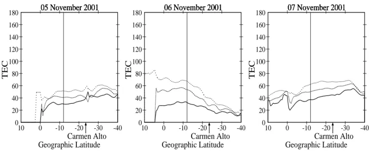
Fig. 10. Total electron content (x106electrons cm−2)along American longitude sector, derived from the GPS phase fluctuations for 5–7 November 2001, at 06:00 LT (solid line), 07:00 LT (middle line) and 08:00 LT (dotted line). During this time period, enhancements were observed in the dayglow emissions on 6 November (see Fig. 7). Magnetic equator is shown as a vertical line. Carmen Alto is located at approximately 23.16◦geographic latitude as indicated by an arrow. It can be seen that the TEC on 6 November did not show any increase corresponding to the increase in dayglow emissions. Actually, a factor of 1.5–2 smaller TEC was measured on this day compared with the quiet day, thus indicating no role of electron densities in the observed dayglow emission enhancement. Hence, it is suggested that a possible increase in the neutral densities be responsible for the rise in the observed dayglow emissions on this day. Also, the asymmetric nature of the TEC distribution with respect to latitude on 6 November indicates the presence of strong equatorward winds that bring neutrals from the high latitudes.

4 Discussion and conclusions

To understand the cause for this morning emission enhance-ment on 6 November, let us examine the production and loss mechanisms for the red line dayglow emissions discussed above. It can be seen that an emission enhancement can be caused by either an increase in the electron and the oxygen densities, or a decrease in the N2density, or changes in the

neutral and electron temperatures, or an enhancement in pho-toelectrons flux or an enhancement in solar UV photons. At any given latitude, the solar photons vary only with the SZA, sunspot number and solar cycle. Hence, one would not ex-pect any short jump in them to cause dayglow emission en-hancements through a photo dissociation mechanism. Simi-larly, photoelectrons are not expected to vary abruptly during the course of the day. The parameter that usually shows most short-term variations is the electron density. Unfortunately, there is no digisonde at Carmen Alto to obtain electron den-sity information. However, GPS-based TEC measurements were available for the South American sector. Figure 10 shows the TEC obtained from this chain for 5–7 Novem-ber at 06:00, 07:00 and 08:00 LT, which correspond to the time period during which large emissions were observed on 6 November. The x axis in these figures shows geographic latitude with magnetic equator indicated by a vertical line. The y axis shows the TEC. The location of Carmen Alto is shown with an arrow in all the three plots. The solid line represents the TEC variation at 06:00 LT. The variations at 07:00 and 08:00 LT are shown by the middle and the top

dot-ted lines, respectively. When one compares the TEC data on all the days at Carmen Alto during these times, it can be no-ticed that the disturbed day (6 November) does not show any increase in TEC. In fact, the 6 November TEC shows lower values over Carmen Alto when compared against the quiet days for all times under investigation. Hence, this rules out the possibility of an electron density increase contributing to the observed dayglow emission enhancement. Also, it is in-teresting to note that there is a significant inter-hemispheric asymmetry in the 6 November TEC data, with lower TEC in the Southern Hemisphere compared to the Northern Hemi-sphere. It is known that owing to the ion-neutral collisions, plasma is dragged along with the neutral winds. However, as the plasma is tied to the magnetic field lines it is trans-ported along the magnetic flux tubes to the opposite hemi-sphere and would be recorded as an increase in the TEC measurements in that hemisphere (Rishbeth, 1967). Hence, the inter-hemispheric asymmetry is an indication of strong neutral winds blowing from the hemisphere with lower elec-tron densities to the one with higher elecelec-tron densities. This asymmetry in the TEC persisted on 6 November until at least 13:00 LT.

The only other parameter that can produce the observed dayglow emission enhancement is the short-term variation in the neutral densities. From satellite measurements it is known that neutral densities increase in low latitudes during geomagnetic storms (for example, Hedin et al., 1977; Mayr et al., 1978; Burrage et al., 1992; Prolss, 1993; Burns et al., 1995). This redistribution is caused by transport of the

D. Pallamraju et al.: Magnetic storm-induced enhancement in neutral composition 3249 neutrals (Mayr et al., 1978; Prolss, 1980) from the hot

po-lar latitudes to the colder low and equatorial latitudes and by TADs (Prolss, 1993; Fujiwara et al., 1996; Balthazor and Moffet, 1997). An essential feature of such a TAD is that it carries equatorward-directed winds along with it. Unfor-tunately, simultaneous neutral wind data from low latitudes are not available for comparing the neutral dynamical vari-ations on the quiet and disturbed periods, as the days being discussed are close to the full-Moon phase (full moon night was 1 November). However, the inter-hemispheric asymme-try in the TEC data on 6 November, as shown in Fig. 10, can be seen as an evidence of the existence of strong equator-ward winds on this day. Further, there is ample evidence in the literature to show that the measured and modeled winds, and TADs during storm time show large equatorward veloc-ities (e.g. Fujiwara et al., 1996; Zhang and Shepherd, 2000; Emmert et al., 2001). Zhang and Shepherd (2000) reported WINDII measured winds of 650 ms−1_{at 200 km in the}

po-lar region for a storm with Kp=7.7. The wind-strengths

re-duce as they propagate towards the low and equatorial lati-tudes (Emmert et al., 2001). The wind strengths also increase with an increase in the intensity and the duration of the mag-netic storm. Furthermore, TADs generated during magmag-netic storms propagate with high velocities from the polar to the equatorial-latitudes, and depending on their strength, they are also capable of propagating to the opposite hemisphere (Fu-jiwara et al., 1996; Balthazor and Moffet, 1997). There is a good temporal correlation between the magnetic storm activ-ity at high latitudes and the increase in neutral gas densities at low latitudes (Prolss, 1993; Fujiwara et al., 1996; Balthazor and Moffet, 1997). Simulation results show that the equator-ward propagation speeds can easily be 650 ms−1_(Fujiwara

et al., 1996) and these wave activity effects can affect low latitude neutral composition within 1–3 h of the storm sud-den commencement time, before propagating to the opposite hemisphere. In the absence of direct wind measurements dur-ing the period of our observations, we assume that similar TADs and winds existed during the 6 November storm pe-riod. As the Kpwas 9−for 6 h and 7 for the following three

hours on 6 November (Fig. 1), which is much greater than the indices for the cases discussed in earlier works, it is fair to assume that the wind and tidal strengths on 6 November are similar in magnitude to the measurements and simula-tion results reported earlier. Hence, we believe that the day-glow emission enhancement seen in the HIRISE measure-ments from 05:30–08:30 LT (10:15–13:15 Universal Time; UT) is a direct result of such an increase in the neutral densi-ties over low latitudes.

It is known that O/N2 changes at different latitudes

dur-ing magnetic storms, which, in turn, alters the ionized gas densities. Large electron densities have been measured with an increase in the O to N2ratio (Mayr et al., 1973; Prolss,

1980). But the variation of OI 630.0 nm dayglow emissions versus the O to N2 ratio is a complex relationship as the

reaction rates are altitude dependent. One needs to model the emissions with varying compositions. Melendez-Alvira et al. (1995) and Witasse et al. (1999), respectively

pre-sented the modeled sensitivity of 630.0 nm twilight airglow and dayglow to [O2], [N2] and [O]. They showed that an

in-crease in O density by a factor of two inin-creases the peak vol-ume emission rate by around 20% through the photoelectron impact mechanism (Witasse et al., 1999). Similarly, dou-bling [O2] can increase the total O(1D) production by at least

60% through photodissociation and dissociative recombina-tion mechanisms (Melendez-Alvira, et al., 1995). Decrease in the N2density by a factor of two increases the red line

volume emission rate due to a reduction in quenching (L1) by about 15% (Solomon and Abreu, 1989; Melendez-Alvira et al., 1995). Thus, the sensitivity of the dayglow emission rates to changes in various neutral species is interrelated and is very complex. Hence, in the absence of simultaneous ob-servations of the altitude distribution of the neutral composi-tion during this storm, it can only be inferred that the increase in observed emissions are most likely due to a significant in-crease in the neutral densities over low latitudes during the 6 November storm. The decrease in the observed emissions around 09:00 LT on the disturbed day can be attributed to the decrease in mass transport of neutral species, due to a de-crease in the storm strength from Kp=9− to Kp=7 in 9 h.

This is commensurate with the measurements (Emmert et al., 2001) that showed a decrease in the equatorward wind strengths with the decrease in the storm strength.

5 Summary

OI 630.0 nm dayglow measurements during a severe mag-netic disturbance (6 Novemeber 2001, Dst=−300) from

Car-men Alto, a low geomagnetic latitude location, revealed a factor of 2–3 increase in emission brightness in the morning hours (05:30–08:30 LT) compared to those on the adjacent quiet days. The cause of these emission enhancements at low latitudes is interpreted to be due to an increase in the neutral densities brought in from high latitudes as a direct ef-fect of the geomagnetic storm. The ground-based dayglow measurements during storm times are therefore a very useful tool in understanding the spatial and temporal effects caused by the magnetic disturbances in the thermosphere. Of the two quiet days presented in this case study, the optical measure-ments on 5 November show weak EIA development followed by no post-sunset ESF occurrence, while 7 November shows a strong EIA development followed by the post-sunset ESF onset.

Acknowledgements. We thank J. Araya for his help in the field

sta-tion and T. Pedersen for supporting the operasta-tion of HIRISE. We thank J. Chau for the ionograms from JRO. We also thank S. Basu for useful discussions. This work was supported by NSF ATM-0077678 and ATM-0209796. The work at Boston College was par-tially supported by NSF grants ATM-0243294 and ATM-01123560, and by Air Force Research Laboratory contract F19628-02-C-0087, AFOSR task 2311AS.

Topical Editor U.-P. Hoppe thanks G. Shepherd and another ref-eree for their help in evaluating this paper.

References

Balthazor, R. L. and Moffet, R. J.: A study of atmospheric gravity waves and travelling ionospheric disturbances at equatorial lati-tudes, Ann. Geophys., 15, 1048–1056, 1997.

Burns, A. G., Killeen, T. L., Deng, W., Carignan, G. R., and Roble, R. G.: Geomagnetic storm effects in the low- to middle-latitude upper thermosphere, J. Geophys. Res., 100, 14 673– 14 691, 1995.

Burrage, M. D., Abreu, V. J., Orsini, N., Fesen, C. G., and Roble, R. G.: Geomagnetic activity effects on the equatorial neutral ther-mosphere, J. Geophys. Res., 97, 4177–4187, 1992.

Chakrabarti, S.: Ground-based spectroscopic studies of sunlit air-glow and aurora. J. Atmos. Solar-Terr. Phys., 60, 1403–1423, 1998.

Emmert, J. T., Fejer, B. G., Fesen, C. G., Shepherd, G. G., and Solheim, B. H.: Climatology of middle- and low latitude daytime F-region disturbance neutral winds measured by Wind Imaging Interferometer (WINDII), J. Geophys. Res., 106, 24 701–24 712, 2001.

Fujiwara, H., Maeda, S., Fukunishi, H., Fuller-Rowell, T. J., and Evans, D. S.: Global variations of thermospheric winds and tem-peratures caused by substorm energy injection, J. Geophys. Res., 101, 225–239, 1996.

Fuller-Rowell, T. J., Codrescu, M. V., Moffet, R. J., and Quegan, S.: On the seasonal response of the thermosphere and ionosphere to geomagnetic storms, J. Geophys. Res., 101, 2343–2353, 1996. Hays, P. B., Rusch, D. W., Roble, R. G., and Walker, J. C. G.: The

OI 6300A airglow, Rev. Geophys., 16, 225–232, 1978.

Hedin, A. E., Bauer, P., Mayr, H. G., Carignan, G. R., Brace, L. H., Brinton, H. C., Parks, A. D., and Pelz, D. T.: Observations of neutral composition and related ionospheric variations during a magnetic storm in February 1974, J. Geophys. Res., 82, 3183– 3189, 1977.

Kelley, M. C.: The Earth’s Ionosphere, Academic Press, 1989. Mayr, H. G. and Volland, H.: Magnetic storm characteristics of the

thermosphere, J. Geophys. Res., 78, 2251–2264, 1973.

Mayr, H. G., Harris, I., and Spencer, N. W.: Some properties of upper atmosphere dynamics, Rev. Geophys., 16, 539–565, 1978. Melendez-Alvira, D. J., Torr, D. G., Richards, P. G., Swift, W. R., Torr, M. R., Baldridge, T., and Rassoul, H.: Sensitivity of the 6300 ˚A twilight airglow to neutral composition, J. Geophys. Res., 100, 7839–7853, 1995.

Mendillo, M., Meriwether, J., and Biondi, M.: Testing the thermo-spheric wind suppression mechanism for day-to-day variability of equatorial spread-F, J. Geophys. Res. 106, 3655–3664, 2001. Meriwether, J. W., Heppner, J. P., Stolarik, J. D., and Wescott, E.

M.: Neutral winds above 200 km at high latitudes, J. Geophys. Res., 78, 6643, 1973.

Moffet, R. J.: The equatorial anomaly in the electron distribution of the terrestrial F-region, Fund. Cosmic. Phys., 4, 313-387, 1979. Pallam Raju, D., Sridharan, R., Gurubaran, S., and Raghavarao, R.:

First results from ground-based daytime optical investigation of the development of the equatorial ionization anomaly, Ann. Geo-phys., 14, 238–245, 1996.

Pallamraju, D., Baumgardner, J., and Chakrabarti, S.: A multiwave-length investigation of the Ring effect in the day sky spectrum, Geophys. Res. Lett., 27, 1875–1878, 2000.

Pallamraju, D., Baumgardner, J., Chakrabarti, S., and Pedersen, T. R.: Simultaneous ground-based observations of an auroral arc in daytime/twilighttime O I 630 nm emission and by Incoherent Scatter Radar, J. Geophys. Res., 106, 5543–5549, 2001.

Pallamraju, D., Baumgardner, J., and Chakrabarti, S.: HIRISE: A ground-based high resolution imaging spectrograph using Echelle grating for measuring daytime airglow and auroral emis-sions, J. Atmos. Solar-Terr. Phys., 64, 1581–1587, 2002. Pallamraju, D., Chakrabarti, S., Doe, R., and Pedersen, T. R.: First

ground-based OI 630 nm optical measurements of daytime cus-plike and F-Region auroral precipitation, Geophys. Res. Lett., 31,L08807, doi:10.1029/2003GL019173, 2004.

Pant, T. K. and Sridharan, R.: A case-study of the low latitude ther-mosphere during geomagnetic storms and its new representation by improved MSIS model, Ann. Geophys., 16, 1513–1518, 1998. Prolss, G. W.: Magnetic storm associated perturbation of the upper atmosphere: recent results obtained by satellite-borne gas ana-lyzers, Rev. Geophys., 18, 183–202, 1980.

Prolss, G. W.: Common origin of positive ionospheric storms at middle latitudes and the geomagnetic activity effect at low lati-tudes, J. Geophys. Res., 98, 5981–5991, 1993.

Raghavarao, R., Sridharan, R., Sastri, J. H., Agashe, V. V., Rao, B. C. N., Rao, P. B., and Somayajulu, V. V.: The equa-torial ionosphere, In WITS handbook, Vol. 1., World Iono-sphere/Thermosphere Study, edited by C. H. Liu and B. Edwards, SCOSTEP Secretariat, University of Illinois, 48–93, 1988a. Raghavarao, R., Nageshwararao, M., Sastri, J. H., Vyas, G. D., and

Sriramarao, M.: Role of equatorial ionization anomaly in the ini-tiation of equatorial spread-F, J. Geophys. Res., 93, 5959–5964, 1988b.

Rishbeth, H.: The effect of winds on the ionospheric F2- peak, J. Atmos. Terr. Phys., 29, 225–238, 1967.

Sastri, J. H.: Penetration electric fields at the nightside dip equa-tor associated with the main impulse of the sequa-torm sudden com-mencement of 8 July 1991, J. Geophys. Res., 107, SIA 9-1 to SIA 9-8, 2002.

Sastri, J. H., Niranjan, K., and Subbarao, K. S. V.: Response of the equatorial ionosphere in the Indian (midnight) sector to the severe magnetic storm of July 15, 2000, Geophys. Res. Lett., 29, 1–4, 2002.

Solomon, S. C. and Abreu, V.: The 630 nm dayglow, J. Geophys. Res., 94, 6817–6824, 1989.

Sridharan R., Pallam Raju, D., Raghavarao, R., and Ramarao, P. V. S.: Precursor for equatorial spread-F in OI 630.0 nm dayglow, Geophys. Res. Lett., 21, 2797–2800, 1994.

Valladares, C., Basu, S., Groves, K., Hagan, M. P., Hysell, D., Mazzella Jr., A. J., and Sheehan, R. E.: Measurement of the lat-itudinal distributions of total electron content during equatorial spread F events, J. Geophys. Res., 106, 29 133-29 152, 2001. Walker, G. O., Ma, J. H. K., and Cotton, E. : The equatorial

iono-sphere anomaly in the electron content from solar minimum to solar maximum from South-East Asia, Ann. Geophys., 12, 195– 209, 1994.

Witasse, O., Lilensten, J., Lathuillere, C., and Blelly, P.-L.: Mod-elling the OI 630.0 and 557.7 nm thermospheric dayglow during EISCAT-WINDII coordinated measurements, J. Geophys. Res., 104, 24 639–24 655, 1999.

Yeh, K. C., Franke, S. J., Andreeva, E. S., and Kunitsyn, V. E.: An investigation of motions of the equatorial anomaly crest, Geo-phys. Res. Lett., 28, 4517–4520, 2001.

Zhang, S. P., and Shepherd, G. G.: Neutral winds in the lower thermosphere observed by WINDII during the April 4–5th, 1993 storm, Geophys. Res. Lett., 27, 1855–1858, 2000.