Dispersion of fine sediments in tides

Dispersion of Fine Sediments in Tides

by

Feng Ye

Submitted to the Department of Civil and Environmental

Engineering

in partial fulfillment of the requirements for the degree of

Master of Science in Civil and Environmental Engineering

at the

MASSACHUSETTS INSTITUTE OF TECHNOLOGY

June 1998

©

Massachusetts Institute of Technology 1998. All rights reserved.

Author ...

Department of Civil and Environmental Engineering

May 8, 1998

Certified by. ,,~

...

,

... /..

/..

Chiang C. Mei

E.

urner Professor of Civil and Environmental Engineering

Thesis Supervisor

A ccepted by ...

.

. .

...

Joseph M. Sussman

Chairman, Department Committee on Graduate Students

JUN

021998-OO

JUN 02198

Dispersion of Fine Sediments in Tides

by

Feng Ye

Submitted to the Department of Civil and Environmental Engineering on May 8, 1998, in partial fulfillment of the

requirements for the degree of

Master of Science in Civil and Environmental Engineering

Abstract

A theory on the dispersion and resuspension of fine particles in the tidal wave bound-ary layer above the seabed is presented in Part I. The inviscid flow lying atop the bottom boundary layer is nonuniform due to the existence of a peninsula protruding out of the straight coastline. A constant eddy viscosity model is applied to achieve qualitative understanding. The length scale of the peninsula is assumed to be much smaller than the tidal wave length while much greater than the tidal excursion length. First we describe the derivations by Mei & Chian of the mean flow, effective transport equation governing the long time evolution of concentration distribution and the ex-plicit expressions of convection velocity and dispersivity tensor in terms of the general ambient flow. A numerical scheme is developed to solve the convection diffusion equa-tion. Two computational examples are discussed to illustrate the application of our theory: one for an initial release of particle cloud near a semicircular peninsula over a solid bed; the other for the resuspension over an erodible belt emcompassing the peninsula. It is discovered that nonuniformity of the ambient flow and earth rotation play the dominant role in determining the evolution of particle concentration.

In Part II we examine the flow field in a shallow lake forced by a low-frequency wind. Depth variation over space is allowed and a general depth-dependent eddy viscosity considered. Since the lake is quite shallow and wind period very long, it is found that the vertical structure of flow field forms a lot faster than any change of forcing takes place. For this quasi-steady problem we develop a perturbation theory to describe the free surface displacement and the velocity field. It is shown analytically that the leading order flow and the steady streaming do not depend on the horizontal extensions of a constant-depth basin under a uniform wind. Finally, the response in a rectangular lake of flat bottom is discussed in detail. It is seen that the transient effect of surface oscillation overplays the Coriolis effect for the second order flow and the mass transport results from the interaction between the leading order surface

motion and oscillatory velocity.

Thesis Supervisor: Chiang C. Mei

Acknowledgement

I take this opportunity to express my gratitude to my advisor, Professor Chiang C. Mei, from whom I have learned not only a lot of knowledge in hydrodynamics, but also the approach and attitude to conduct scientific research. I extremely admire his drive and devotion to engineering science. The door of his office opens towards me whenever I want to have a discussion on my research. Without his guidance and encouragement, this research could never have been done.

I gratefully acknowledge my friends in our group who discussed with me about the contents of the thesis, especially Jie Yu and Zhao Cheng. I would like to thank the professors and other graduate students at the Parsons Lab from whom I have learned a lot and with whom I have had these past three years of happy time.

I am also grateful for the financial support by the US Office of Naval Research through Grant N00014-89-J-3128 and National Science Foundation through Grant CTS 9634120.

Last but not least, my parents and sister's love has always been the source of strength with which I am confident to face any challenge.

Contents

I

Dispersion of Fine Particles near a Small Peninsula

1 Introduction

2 Mathematical Formulation

2.1 Tidal wave boundary layer flow ...

2.2 Particle transport . . . . 2.2.1 Governing equation and normalization ...

2.2.2 Effective equation for horizontal particle transport ...

3 Numerical scheme

4 Release of a particle cloud

5 Resuspension and transport of bottom sediments 6 Conclusion

II

Flow Field in a Basin Forced by a Low-Frequency

Wind

13

3 Analytical Solution for a Constant-Depth Lake Forced by Uniform

Wind 88

4 Rectanglar Lake with Uniform Depth 95

5 Conclusion 124

A Fortran program solving the effective transport equation 126

B Proof of the uniqueness 138

List of Figures

I-2-1 Dimensionless complex coefficient H1 (f, Pe) for the mean convec-tion velocity, as a funcconvec-tion of Coriolis number f = 2Q sin 0/w, for

Pe = 1. ... . ... .. 32 I-2-2 Dimensionless dispersivity coefficients as functions of Pe for f =

0.666. Dashed: Sc = 0.1, solid: Sc = 1, dashdot: Sc = 10 .... 34

I-2-3 Dimensionless dispersivity coefficients as functions of f for f =

0.666. Dashed: Sc = 0.1, solid: Sc = 1, dashdot: Sc = 10. .... 36 I-2-4 Weighted depth-average of convection velocity UE in the tidal

boundary layer for f = 0.666 and Pe = 1. . ... . 37 I-2-5 Dispersivity tensor components around a circular peninsula for f =

0.666, Pe=- 1 and Sc =1 ... ... 38 I-2-6 Dispersivity tensor components around a circular peninsula for f =

0, Pe = 1 and Sc = 1 ... 40 I-4-1 Evolution of particle concentration. Cloud center is initially

re-leased at north-east (r' = 1.3, Oc = 450) for f = 0.666, Pe = 1 and

Sc= 1. ... . . ... 49 I-4-2 Off-diagonal dispersivity tensor component E0r around a circular

peninsula for f = 0.666, Pe = 1, and Sc = 1 . ... 51

I-4-3 Evolution of particle concentration. Cloud center is initially

re-leased at north-west (r' = 1.3, 90 = 135') for f = 0.666, Pe = 1

I-4-4 Evolution of particle concentration. Cloud center is initially re-leased at north-east (r' = 1.3, Oc = 45 ) _{for f = 0, Pe = 1 and}

Sc= 1. ... 54

I-5-1 Dimensionless erosion rate around a circular peninsula due to tidal oscillation .. . . . . 58 I-5-2 Evolution of concentration of resuspended particles. Dashed curve

indicates outer edge of the erodible belt. f = 0.666, Pe = 1 and

S c = 1. . . . . 59 I-5-3 Evolution of concentration of resuspended particles. Dashed curve

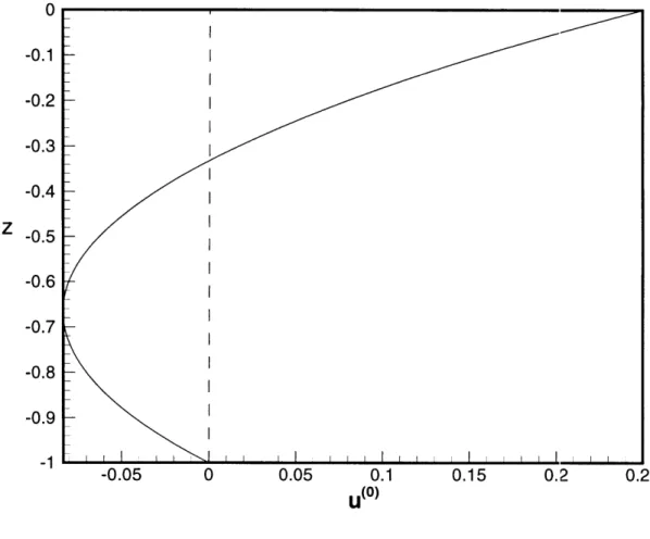
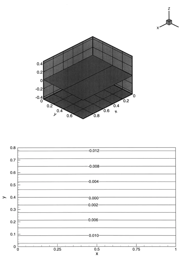
indicates outer edge of the erodible belt. f = 0, Pe = 1 and Sc = 1. 61 II-4-1 Vertical profile of u(O) along the wind forcing direction at t = 0 98 II-4-2 Snapshot of ((1) at t = 0. Upper: surface plot; lower:

equal-elevation lines. ... 102

II-4-3 Snapshot of ((1) at t = 7/4. Upper: surface plot; lower:

equal-elevation lines. ... 103

II-4-4 Snapshot of ((1) at t = 7r/2. Upper: surface plot; lower:

equal-elevation lines. ... 104

II-4-5 Snapshot of ((1) at t = 3r/4. Upper: surface plot; lower:

equal-elevation lines. ... 105

II-4-6 Snapshots of u(1) at z = 0. Upper: t = 0; lower: t = 7/4 . ... 108 II-4-7 Snapshots of u(1) at z = 0. Upper: t = 7/2; lower: t = 31r/4. . 109 II-4-8 z-dependency of the term in u( 1) associated with u( ). ... 110 II-4-9 Flow pattern of u(1) at z = -0.7 and t = -r/4. . ... 111 II-4-10 Snapshots of circulation in xz plane at y = b/2L. Upper: t = 7/2;

lower: t = 37r/4 ... ... 112 11-4-11 Contours of steady surface set-up (((2)) with a wind inclined at

22.50 with respect to the positive x axis. . ... 117

II-4-13 Surface mass transport pattern with the wind making a 22.50 angle

with +x axis ... ... 119

II-4-14 Steady surface set-up due to oscillatory wind along x axis. ... 122 II-4-15 Mass transport pattern in xz due to oscillatory wind along x axis. 123

List of Tables

Part I

Dispersion of Fine Particles near a

Small Peninsula

Chapter 1

Introduction

Sediment transport has been one of the major topics of coastal engineering for a long time due to its signifance to human life. Under the combined action of coastal waves and currents, particles of various sizes are stirred up from the seabed and then carried around. The accumulative effect of this process results in the evolution of the coastline over time. One problem associated with the adverse influence of the coastal sediment transport is beach erosion; structures and facilities installed on the beach are threatened. Another important issue has been brought up by the marine disposal practices of the coastal cities. Where are we supposed to set up the outfall diffusers so that what we want to dispose of can really be disposed without being flushed back to the beach where people live? The flow field must be first investigated prior to any prediction of the spreading of the suspended particles can be made. It is well known that dispersion are more prominent in a shear flow than in a uniform flow with the same discharge. Since shear is significant inside boundary layer and tides are just common phenomena as a driving agent in the coastal flows, we want to study the transport process of fine particles in a tidal boundary layer above the bottom.

Transport of suspended sediments has been investigated for decades. Following the pioneering work by Taylor (1953) on dispersion in pipe flows, a number of authors have explored dispersion of a neutrally buoyant cloud in a horizontally uniform but oscillatory current. Bowden (1965) studied the horizontal mixing in a tidal current. Holly & Harleman (1965) conducted dye-release experiments in oscillatory pipe flow.

Okubo (1967) then pointed out the dependency of diffusivity on the oscillatory period of the flow. For suspended fine particles, Yasuda (1989) discovered that the dispersion coefficient of particles at the stationary stages is dependent on the settling velocity of the sediments and reaches a maximum value corresponding to a critical fall velocity. Despite their success in showing many interesting physical courses, these uniform-tide theories are not adequate in predicting the long time evolution of a particulate cloud with a size comparable to the length scale of a coastline feature, in that case the nonuniformity of the ambient flow becomes prominent.

For the mixing and flushing of tidal embayments in the Dutch Wadden Sea,

Zim-merman (1976, 1977) argued that that the large diffusivity (100 - 1000 m2/s) is due

to horizontal mixing in a spatially nonuniform flow. His work caused scientists' at-tention upon the effect of horizontal variation of topography (shore configuration) on mass transport. Two approaches have been adopted to model dispersion in nonuni-form tides: 1) Based on the estimated depth-averaged flow, the trajectories of a large number of marked fluid particles are computed numerically. A few works followed this Euler-Lagrangian method (Zimmerman, 1986; Awaji et al, 1980; and Signell & Geyer, 1990). 2) The second approach is an Eulerian approach. Young et al (1982) studied an idealized flow field with simple dependence on spatial coordinates and sinusoidal dependence in time. The three dimensional convective diffusion problem was solved to enable the calculation of the effective horizontal diffusivity. In our research we will take the Eulerian approach.

As for the proper form of the eddy vicosity, Sleath (1990) reviewed many depth-dependent models for gravity waves and Soulsby (1990) for tidal currents. In addi-tion, the latter (see Soulsby, 1990, p 531) provided sketches showing that despite the varieties (constant, linear, parabolic, exponential), the resulting first-order velocity profiles do not differ qualitatively. To achieve physical understanding with simple algebra, we shall follow Sverdrup (1927), Mofjeld (1980), Kundu et al (1981) and Fang and Ichiye (1983) and choose the simplest model of constant eddy with no-slip boundary at the seabed.

strongly by nonuniformities due to coastline feature. In Chian (1993) and in an un-published paper by Mei & Chian (1994) an analytical theory has been worked out for the mean flow and the dispersion equation for suspended sediments. After some revisions of their formulas, an effective numerical scheme is developed here for guanti-tative computations. The length scale of the peninsula is assumed to be much smaller than the tidal wave length while much greater than the tidal excursion length. In Chapter 2 we first present the solutions of the leading order oscillatory boundary layer flow and the mean flow at the second order, and then effective transport equa-tion governing the long time evoluequa-tion of concentraequa-tion distribuequa-tion with the explicit expressions of convection velocity and the spartially dependent dispersivity tensor in terms of the general ambient flow. A numerical scheme is developed in Chapter 3 to solve the convection diffusion equation. ADI method is applied along with boundary conditions of second order accuracy with respect to the time step and mesh den-sity. Two computational examples are discussed in Chapter 4 and 5, respectively, to illustrate the application of our theory: one for an initial release of particle cloud near a semicircular peninsula over a solid bed; the other for the resuspension over an erodible belt emcompassing the peninsula. It is discovered through this research that nonuniformity of the ambient flow and earth rotation play the dominant role in determining the evolution of particle concentration. The analysis is an extension to our earlier works on gravity waves over a nonerodible seabed (Mei & Chian, 1994) and an erodible seabed (Mei , Fan & Jin 1997), without Coriolis effects.

Chapter 2

Mathematical Formulation

Transport of suspended sediments in coastal waters near a small peninsula is con-sidered. The Eulerian approach is used to study dispersion in tidal flows affected strongly by nonuniformities due to coastal topography. We first find the flow field in order to study the transport of particles in the tidal wave boundary layer. Besides the obvious periodic tidal wave oscillation, a steady streaming is generated as a result of nonlinear terms.

2.1

Tidal wave boundary layer flow

Our main assumptions are as follows. The topographical length scale is assumed to be greater than the tidal excursion length, so that flow separation is not important. Let h denote the sea depth, ro the horizontal size of the coastal topography, A the

typical tide amplituide, w the tidal frequency, and U - AJSgh/h the typical horizontal

flow velocity. Just above the sea bed, an oscillatory Ekman boundary layer of the thickness 6 = O( w) is expected to develop, where v, denotes the eddy viscosity

of momentum. The various scales involved in this problem are assumed to satisfy the following constraints:

6 6 h

E < 1, - < 1 - < 1, kro <1 (I.2.1)

They mean, respectively, that the tidal excursion is small compared to the island size, the Ekman layer is totally submerged near the sea bottom beneath the inviscid zone, the sea is shallow, and the topographical length scale is small relative to the tidal wave length 27r/k. Resuspension of fine particle from the seabed is modelled by the usual empirical formula that the erosion rate is a function of the shear stress at the seabed (Krone, 1962; Patheniades, 1965).

The conditions of (1.1) are easily met. Taking for estimate the tidal amplitude

A = 1.75 m, average depth h = 30 m then U = AVg-/h = 1 m/s. Let the tidal period be 12 hours so that w = 2r/12 (1/hr)= 1.45 x 10-4 _{(1/s), and the radius be}

ro = 50 km, then e = Ul/(wro) = 0.138 and is small.

To help guide the estimate of order of magnitude of the eddy viscosity we use the usual assumption (Soulsby, 1983)

Ve = Nu*z (1.2.2)

where n = 0.4 is the Karman constant and u. = Tb/P is the friction velocity which depends on the local shear stress at the bed. Taking the typical value u* = 2.5 cm/s as an estimate (Soulsby, 1983, p 196) we then get for a tidal boundary layer of depth 10 m, ve = 0.05 m2/s which is much greater than that of the molecular viscosity of water.

Let us set up the coordinates with the vertical axis fixed on the sea bottom and pointing upward. Using the external inviscid flow equation to eliminate the pressure, with the second assumption in (1.2.1), the boundary layer equations can be written:

0u

au

at az az2

Ut

= - + U, VUI + fx UI, (I.2.3)

where u = (u, v) denotes the horizontal velocity vector, w the vertical velocity

com-ponent, ve the eddy viscosity, and f = 2Qsinok is the local angular velocity of the earth rotation, with Q = 27r/day and ¢ being the local latitude. U, denotes the

horizontal velocty of the inviscid flow field just outside the boundary layer, U1 = Re[Uo(x, y)e-i t 1 (Uoe-iwt + U*eiwt)

2 0

where asteriks signify complex conjugates.

The first assumption in (1.2.1) permits one to expand the velocity in the boundary

layer as

u = u (1) + u(2 ) + ...

where the superscripts indicate the order of magnitude in powers of E. At the leading order the horizontal momentum equation reads

at

In complex form, with overbars denoting the complex variables,

UI = UI + iV = Be-iwt + Ceiwt,

1

B = (Uo + iVo) C = ₂(U + i Vo*) .

Due to linearity, we may split the solution into two components, namely,

(1) = U(1) + iV) =91B + U1C,

(1.2.8)

(1.2.9)

(I.2.10) (1.2.4)

O-UB 02 1B

ait + 2iQ sin U1B - Ve BOZ = iw(f - 1)Beiwt, (I.2.11)

i + 2i sin ic - ye = iw(f + 1)Ceiwt. _(1.2.12)

at

az2

Note that on the right-hand side of Equation 1.2.11 the factor f - 1 with

f = 2Q sin 0/w = Coriolis factor. (1.2.13)

will change sign when f varies accross unity. This further causes the direction of the forcing to turn opposite and the magnitude of the forcing stops increasing and begins decreasing or verse vice. The linear response to this variation of forcing is still smooth. But due to nonlinearity, we can expect a discontinuity accross f = 1 in the f-derivatives in both second order streaming and transport parameters. Let

UIB = FB(()Be - i t ULc = Fc()BeiWt, (1.2.14) with

z

[o-~ + 2i(1 - f)](FB - 1) = 0, (I.2.16)

092 [Q-~ - 2i(1 +

f)](Fc

s = (1 + i)3, if

f

U(1) = Re[(UoFI - VoF 2)e-it], (1.2.21)

V(1) = Re[(UoF2 + VoFi)e-iwt], (1.2.22) in which F = 1 - 1(e-s + e-q), (1.2.23) F2 = (e-s - e-qC), (1.2.24) 2 where q = (1 - i)a. (1.2.25)

As has been shown by Buchwald (1971) that under the last two assumptions in (1.2.1), the inviscid tidal flow (U1, VI) can be described essentially by a two-dimensional, quasi-steady velocity potential, while the vertical velocity component is negligible. In particular,

au,

_ 9 = O(kro)2

(

ax

It follows readily from continuity that the vertical velocity in the boundary layer is of the order

- (kro )2 _(1.2.27) ro ro

and negligible (Lamoure & Mei, 1977). As a further consequence the spatial factors Uo and V are in phase and may be taken as real quantities with respect to i. Based on these Lamoure & Mei (1977) have solved the approximate momentum equation at the second order, O(C),

dU( 2 )

2U ( 2 ) ₁

+t

+

_D

The period-average of u2 gives the Eulerian streaming induced by Reynolds stresses

in the tidal boundary layer. Using real notation, the second order induced streaming is given by

1

(U(2)) = ReHE)+ Uo2 - Im HE (1.2.29)

(v(2)) = 2 Im HE() z IUo2 + Re HE( ) IU012 0 (1.2.30) where

IUo0 = (IU02 + IV012)1/2, (1.2.31)

angle brackets denote time averages over a tidal period, and HE( ) marks the vertical variation of Eulerian streaming in the boundary layer

2 (q2 - C2 q2 - C2 4a2 _ C2 1 _ 1 _ 1 -2 / q2 - C2 q2 _ C2 4a 2 - C2 1 + -{a -+ 3, q - s} (1.2.32) 2

The expression in the second pair of braces is obtained from the first pair by the indi-cated change of parameters. This result has been derived and discussed by Lamoure & Mei (1977).

2.2

Particle transport

A dilute cloud of fine particles in the tidal wave is considered. It can be either released from a dredge boat or resuspended locally from an erodible bed. In general the sediment size is distributed over certain range. Since for a dilute cloud, interaction among particles is negligible, one can divide the size distribution into a discrete set of particle sizes, each of which is characterized by a fall velocity wo. After analyzing the concentration of each size, the evolution of the entire cloud can be obtained by linear superposition. In the sequel only one size is considered.

2.2.1

Governing equation and normalization

We first give reasons that the inertia of sufficiently small particles can be ignored. The ratio of the relaxation time 7 for a particle to adjust to the ambient mean flow to that of the tidal wave period can be estimated by

WT = (1.2.33)

3CDAU

(Bagnold, 1957) with d, pp, CD and Au being respectively the diameter and density of the particle, the drag coefficient and the representative initial velocity difference between a particle and the ambient fluid. With CD = 0(1) and Au = 0(1) m/s, this

ratio is about O(10- 5) for d = 0(0.1) mm = 100pm (fine sand), and is very small so that the particles are essentally inertia-free. In a turbulent field, fine particles can also be considered inertia-free relative to turbulent fluctuations if they are small compared to the Kolmogorov length, k = (v3u~e/') 1/ 4, which is the smallest length scale of viscous eddies, i.e.

d

-< 0(1) (1.2.34)

fk

where where

e

Tb stands for the bed shear stress. Estimating with ve = 0.001 m2_{/s and thus a tidal} boundary layer thickness of £ = 0(3) m and u, = 0(0.01) m/s, we have ek = 0(1) mm

which is also much greater than the particle radius 0(0.1) mm. We shall, therefore, ignore the velocity difference between the particle and its surrounding fluid.

Let D and Dh be the vertical and horizontal eddy mass diffusivities respectively. The convection-diffusion equation for the concentration C of a dilute particle cloud can be approximated by

aC OuiC O(w -

wo)C

02C

+ + = Dh + D (1.2.35)

Ot

Oxi

Z

where i = 1, 2 corresponding to the two horizontal coordinates.

over an erodible bed, the net rate of erosion or deposition of cohesive sediments is related to the excess of bed shear stress above a threshold stress. In its simplest form it reads

- woC - D if (1.2.36)

z

J

where Tc > d and

D = OidWdC (1.2.37)

represents the rate of deposition, Wd is the deposition velocity, ad is an empirical

coefficient no greater than unity, and

8 = E(bl - 7T) (1.2.38)

represents the rate of erosion while E is another empirical coefficient. Normally Td ranges from 0.03 n 0.15 N/m 2 for various types of sediments while T. lies between 0.15 N/m 2 and 1 N/m 2, see Tables 11.3, 11.7 and 11.8 in Van Rijn (1994). The surface

layer of the sea bed is usually covered with partially consolidated or unconsolidated particles for which Tc is considerably less than the bed shear stress in the tidal wave boundary layer, namely, 7b > 7.. Thus we shall neglect T. as well as Td(< Tc)

Consequently we shall ignore deposition and approximate (1.2.36) by

DOC

- (woC + D ) = S ETb|, z = 0. (1.2.39)

It should be stressed that inculsion of the small effects of deposition is only cumber-some but not difficult. In a steady turbulent flow, the condition for particles remaining in suspension without deposition is wo/1U, < 0(1) (Batchelor, 1965) where u, and K

are the bottom shear velocity and the Kirmin constant, respectively. As an estimate let us take u, = 0(0.01) m/s, then the above condition by Batchelor is satisfied for

wo < 0(0.004) m/s which corresponds to a sand size d = 0(0.1) mm or finer.

Because the particles are heavier than water, siediment concentration is expected to be localized boundary layer where the particles are kept in suspension by the flow

turbulence. Hence we assume that C vanishes at the upper edge of the boundary layer,

C = 0, z -+ 00. (1.2.40)

There are three vertical length scales pertinent to the boundary layer,

6S = D/wo, 6, = 2ve/w, 6c = 2D/w. (I.2.41)

Here 6, denotes the thickness of a steady concentration layer resulting from the set-tling of particles and the upward turbulent diffusion, and 6, and 6 are the boundary layer thicknesses corresponding to momentum and mass transport, respectively. For generality we shall assume that all three scales are comparable to one another and therefore characterized by a single scale 6, i.e.,

0(6) = 0(6,) = O(6S) = 0(6), (1.2.42)

and thus the Schmidt number is of order unity,

Sc = ve/lD = (6,/6j)2 = O(1). (1.2.43)

Two small length ratios are crucial in this study. Compared to the horizontal dimension of the peninsula,

U

/g-E- U - A , (1.2.44)

wr0 ro is a measure of the tidal excursion length, and

6 Dh

S= 0i

,

where

/

O(0) = O(E), the consequence of which is that horizontal turbulent diffusion will

Let us introduce the normalized variables as follows t* i rox, z =z*, t = _W, C = -CO*, 6 i = Uui, w = w*. ro

In dimensionless form, the governing equation reads, with the asterisks omitted for brevity,

0C +

(uiC)

Ot xi

dt 8i + + z -[(-Pe + Ew)C] = Oz2c

where Pe = wo6/D is the particle Peclet number.

As shown by Mei, Fan & Jin (1997), the characteristic concentration Co can be estimated by balancing the rate of erosion and the net horizontal flux by Eulerian

streaming within the boundary layer, namely,

0C

E

6-

ax (1.2.48)

where UE denotes the scale of the Eulerian steady streaming. From (2.15) and (2.16) we can estimate

where U = AV/l/h for long waves in shallow seas, hence,

The shear stress on the sea bottom can be estimated from the boundary layer theory

_ \/pDU _ V/gpDA

U - 6

V-pEDwr v h

Co ~

_AS2vrd

(1.2.46) 2 02C (1.2.47) UE = O(2 wro (1.2.49) 6A2 gCo whro (1.2.50) therefore (I.2.51) (1.2.52)

Using this, the normalized boundary condition at the seabed reads aC 2 J2 - Pe C - =- (1.2.53) =z wDro2ITbI where U252

A

This scale estimate is consistent with field observations by Huhe & Yang (1996), Yu

et al (1995), and cited by Mei, Fan & Jin (1997).

In the present problem there are two time scales: One is w-1 = T/2r = O(62/D),

which characterizes the vertical diffusion across the boundary layer .The other is the time scale for horizontal diffusion or convection across the peninsula, O(ro/Dh). The ratio between these two time scales is O(f32) = 0(e2). Accordingly we may introduce a slow time variable T = c2t.

2.2.2

Effective equation for horizontal particle transport

After those scaling and order estimates then we return to physical coordinates by keeping the order symbols in order to mark the relative magnitudes. Thus we have

dC

0(uiC)

- (woC + D

az)

C -+ 0, z > . (1.2.57)

As in Mei & Chian (1994) and Mei et al (1997), we employ multiple-scale expan-sions

At the leading order 0(1), the equation is quasi-steady and homogeneous,

z _{woC(o) + D =O 0. (1.2.59)}

Oz \ z /

subject to the homogeneous boundary conditions

woC (O) + D = 0 (1.2.60)

C(o) = 0 z = 00 (1.2.61)

Thus, the solution is

C(O) = (xi, T)e-Pe. (1.2.62) represents the time averaged concentration whose dependence on xi, T through the factor C(xi, T) is yet unknown.

At O(E), we have the equation for the concentration fluctuation C(1) from the mean,

C

a

subject to the same boundary conditions (1.2.60) and (1.2.61). In Equation (I.2.63) we have dropped the term walC (0_{)/Oz because wl is negligible near a small peninsula,}

as pointed out before in Section 2.1. Let

C(1) = Re Clle- iw t , (1.2.64)

Using the solutions for uli as given in Equations (1.2.21) and (1.2.22) , the formal solution for C(O) and the boundary conditions for C(1), we obtain

C11 = - [(RUo - R2Vo)eA1Pe+ R3Uoe-PeC

+ R,(Uo - iVo)e-AaPe + R(Uo + iVo)e-_AgPe]a

1 aO

with

Sc Ap-1 A -1

R,= SC-Aa - 1 - + Act 1 (1.2.66)

Pe2_(A

1 + 1)

[(A

iSc(As - Ap) 1

Pe2(A1 - A2)

[-(A,

+ A2 + (1.2.67) (A2 + Aa)(A2 + A,3)(A + 1) ' 2Sc Pe2(1 + A1)(1 + A2)' (.2.68) Sc Rt,p = _Pe2 (1.2.69)

(Al + A,,) (A2 + Aa,p)'

Ac = (1 - i)a/Pe + 1, Ap = (1 - i)f/Pe + 1, (1.2.70) A1,2 = -1(1 Frl) 1 2it 2, (1.2.71) (1 + N 4_{) 1} r,22 ], (1.2.72) N = Pe = Sc = (1.2.73) Pe D' D'

Note that Pe is the particle Peclet number which increases with the particle fall vel-coity, hence its diameter. Sc is the Schmitt number measuring the ratio of momentum and mass diffusivities.

At O(I2), C(2) is governed by

C(2)

Taking time average and integrating across the boundary layer, and noting that the concentration vanishes at the top of the layer and that the vertical velocity must be

zero at the bottom, we get the effective transport equation for C: = (u 1)C(1)) Ox i 020 + DhF + E(1bl). 8xioxi

where overbars denote vertical integration across the boundary layer and F = e- P e.

Using the results (1.2.21), (1.2.22), (1.2.65), and (1.2.29), we finally have the following effective transport equation:

aC D

+ x(UEiC)

T

8xi

OC

Oxj

EPe(Tbl)

+ ₅

The effective convection velocity UE has the components

UE1 UE2

=

[

ax

(IUo2+ IV012)Im(H1)],

H1= G(a) + G(3)

G(a) = Pe

[c +

q + Pe + 3(a)q* + Pe

4(a2 + f)i 4(a 2- _f)i

8-2 - _4fi'

=2(a)

-4(a 2 + f)i' 1

I3(a) = _{4(a- f)i'}

1

8

8

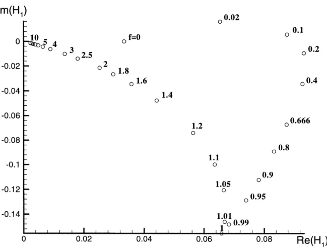
The polar plot of complex coefficient H1 is presented in figure I-2-1 for a wide range

oC

a

[(u2))F(]

Im(H,)

_0.02

Re(H,)

Figure 1-2-1: Dimensionless complex coefficient HI(f, Pe) for the mean convection velocity, as a function of Coriolis number f = 2Q sin q/1, for Pe = 1.

of f.

Referring to (1.2.77), the effecive convection velocity field is the weighted depth-average of the Eulerian streaming velocity, proportional to the Reynolds stress im-posed by convective inertia in the inviscid flow above the boundary layer. The com-plex factor H1 combines the effects of shear and the concentration variation F inside

the boundary layer. The ratio Im Hi/Re H1 = tan- 1 OH gives the angle OH between

the driving external Reynolds stress and the convection current, as a result of earth rotation. Thus for f = 0, ImH1 = 0 so that the angle is zero. But as f increases

to 1, the convection velocity is inclined at 670 clockwise from the external Reynolds stress. For f increasing past unity, the angle OH decreases again.

The dispersion tensor is in general non-symmetric and has the components :

1

Exx = -Re[H 41IUoI2 + H42 Vo2 + H43U*V + H44Vo*Uo], (1.2.84)

Ey, =

-Re[H41Vo

4 2Uo 2 -H44U*V -H43Vo*U], (1.2.85)

Ex, = -Re[-H 431Uol2 + H441Vo2 + H4 1UVo - H42UoV], (.2.86)

Eyv = -Re[H 43Vol2 - H44

1U1

H41 = -- [RIS,(A1) + R3S1(-1) + RaS1(-Aa) + RpSI(-A)], (1.2.88)

1

H42 = -- [R 2S2(Ai) + iRaS2(-Aa) - iRS 2(-A)], (1.2.89) 2

H43 = -[R2S1(A1) + iRjSij(-Aa) - iRpSj(-A)], (1.2.90)

H44 = [R1S2(A1) + R3S2(-1) + RaS2(-Aa) + RpS2(-A)], (1.2.91)

2a₂Pe - (s* + q*) 1 (.2.92) 2(aPe - q*)(aiPe - s*) ai

i(s* - q*)

2(aiPe - q*)(aiPe - s*)'

in which {al, a2, a3, a4} = {A1, -1, -A 0, -Ap}. represent the integrated effects of

the vertical variation of the fluctuating velocity and concentration inside the Ekman boundary layer, hence they are functions of f, Sc and Pe. Since Uo, Vo are in phase and can be taken as real numbers, only the real parts of H4i are needed, and are plotted in figure I-2-2 as functions of the Peclet number Pe for f = 0.8 and three different values of Sc.

In the northern hemisphere, this correspond to the latitude of 53'. All of these coefficients except Re H44 achieve their greatest values near Pe - 1. Dependence of

0, m0 O . II

'-Re(H

₎

Re(H

₎

(a)

(c)

_Pe

Re(H

₎

Re(H

₎

(d)

Pe

these coefficients on f is plotted in figures I-2-3 for Pe = 1 and three values of Sc. Discontinuity in slope at f = 1, i.e., w = 2Q sin ¢ is a common feature which is caused by the change of sign in (1.2.93).

The effective convection-dispersion equation can be written in conservation form

+ 0, (1.2.94)

OT Ox,

where

0C

ji = UEiC - (Eij + DSj) - (1.2.95)

is the particle flux vector.

Under the present assumption of constant depth, the shore must be a vertical cliff normal to which there is no horizontal flux i.e.,

in= -UEiC- (E + D6) ni = 0 (1.2.96)

For presentation of numerical results, it is convenient to renormalize the variables as follows

t = T' 2 _,

= r'x, C= C'Co

2 _U2

UE = UEir , (D, E) = D', E) (1.2.97)

where the concentration scale depends on the problem to be specified later. The effective convection-diffusion equation then becomes

00' a (( aO(UELC') ±D

)

OT- + O = (E i + D '_f) _{+ '.}

(1.2-98)

In the following sections we shall limit our discussion to a semicircular peninsula. The first order spatial dependence of the inviscid velocity field is then simple and is

Re(H

₎

Re(H

₎

f

Re(H

₎

Re(H

₎

2--1 ₀

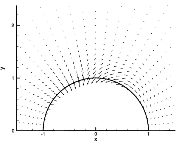
1

Figure 1-2-4: Weighted depth-average of convection velocity UE in the tidal boundary

layer for f = 0.666 and Pe = 1.

identical to that for uniform flow passing a circular cylinder

cos20 sin20 (1.2.99)

Uo =U'T = (1 - 2 ), Vo = - (sin2 ) (I.2.99)

where r' = r/r. The mean velocity of Eulerian streaming is shown for

f

In figure I-2-5 we display the cartesian components of the dispersion tensor Eij for the semi cirular peninsula, for

f

x x 0 0. 0L00 To ao~- 41. 90 01 00 0~0 00 9 0,0 91~ 0.) 0 x~~ L-L -0 0 0 a x-L0 97100 xj L

For f = 0 these components are symmetrical with respect to the y axis, as shown in figure 1-2-6. For rough estimate let us take again U = 1 m/s and w = 1.45 x 10-4 1/s. From figure I-2-2 the typical value of Eij near the peninsula is 0.05, therefore the dispersivity is of the order Eij - 0.05U2/w = 345 m2/s which is consistent with

(a) _Exx "tII II I4. C+ 0 0 0 C+ 0 F-CD c, 0 II 03 (c) Exy -1 o 1 -1 0 (b) Eyy (d) Eyx

Chapter 3

Numerical scheme

For computational convenience, we first split the dispersion tensor Eij into symmetric

Dij and antisymmetric Aij parts and rewrite the governing equation (1.2.98), with

primes omitted, in the following form:

OC ,DOC ,DC

a+

_c

+

-Ox

_8z

axay

D -- Dyx = (Exy + Ey)

- [Re(H4 3) + Re(H4 4)](V 0o 2 2

+Re(UoVo*) [Re(H4 1- Re(H4 2)], where (1.3.1) and Dx = Exx (1.3.2) (1.3.3) (1.3.4) SDy = Eyy, -

u012)

= -A+ = (Ey+E) 1

= [Re(H44) - Re(H43)]0(IVo 2 + IU012) -Im(UVo)[Im(H 41) + Im(H42)].

Equation (1.3.1) is then transformed in polar coordinates, handy for our circular peninsula, 0C ,OC

+ u'

+ u'

_7C

+ v'sin - sin Cos + sin20,

r r r

1

u/ = -u'sin0 + v'cosO - -(Dxxsin20 + D sin20 + 2Dxcos20), r

Dr = DXXcos20 + D,,sin20 + Dxysin20, Doo = Dxxsin20 + DyycOs 2_{0 - Dxysin20,}

1

Deo = 2 sin20(DY - Dxx) + Dxycos20.

(1.3.8)

(1.3.9)

(1.3.10)

(I.3.11)

(1.3.12)

As the radial variation near the peninsula is expected to be very rapid, we intro-duce the stretching: r = exp(27r(), and r = 09/r so that Equation (1.3.7) becomes

C D02C + uac + YC = D(C a 71 l aa _{_j} 02C + D 02Off2 02C + 2DC,7 + _, 10 ir) where u( = u'.so + 2rs Drr, D, = 4s Doo, U = 2u/'so, = 27rr (1.3.6) with (1.3.7) 0C OC

a

+ uC

For this initial value two dimensional convection-dispersion equaiton, we adopt the ADI Method (Alternating Direction Implicit Scheme) which is unconditionally stable and thus allows us to use reasonably large time steps, with second order accuracy,

O(At2, A(2, A712). With each time step At, we solve implicit one-dimensional problem for

C

(-sweep:

Cn+1 2 C Cn n/ 2 n+1/2 ~ - C Cj+1/2 C

23 + i+1, ,i-1j ,j+1 ,j_ - + c

At/2 +u,i 2AC (ni 2Ar 2

2

,++,

+

c+

,-

)/2A2

(c

+

c-

,-

)/2Anr

+

fg,

(I.3.17)

and i-sweep:

C±1 _n+1/ 2 + n+1/2 -) n+1/2 Cn+1 -_ +1 C+1/2 CC + 1

3 . +i+1,j i-i,j +i,j+1 i,j-1 +

j-At/2 , 2,j 2A 2

=D f' (Cn+l/2 Cn+1/2 2C ~+1/2 D ( cn++ + c + xn+l 1 2C+ +)

j n+1/2 +1/2n+1/2 n+n+1/2 ,

_i ,lj+l C +l 1 )/2A - (C- + i-l ₁)/A + . (.3.18)

+2Dc,/ 2 2A 2AC

These, respectively, give

a ,lC +_/2

_{- 2}

1n+1)2

!

(I.3.19)-2

l W-l,j a-- + 2 2+l,j = re,

and

at7 C n +l 2 +1 as+1 _n+1/2, (I.3.20)

1 ,j-1 l 2- t ij 3 / j+1 -in which

al , = -bl,,, - b3, ,

a3(, = blC,n - b3,l, bo = 2A(Ar/At bl( = U(Aqr/2, b177 = _u,A\(/2, b2 = A(Aqr/2, b3( = DccA?/(, b37 = D nA(/7, bac = D,/2, (1.3.21) r" = (bo - b2 - 2b3()C + (b3 - bl)Cn+1 + (b3 b)Cn+-1 2+ + Ln+ -+1/2 = (bo - b2 - 2b )Cn+ /1 2 + (bs - b c)Cz+ 2 + (b₃( + bl()Czi 2 ±ij + 1/2 On,n+1/2 = b3 (C, +12 -

C,1/

Now let us consider the boundary conditions. At the open sea (i = mm), as-suming that the computational domain is sufficiently large given that the convection transports particles toward the peninsula, and therefore, the concentration vanishes practically, namely,

Cmm,j = 0. (1.3.23)

At the rim of the peninsula, r = 1, it follows from (1.2.95)

DC dC

Fr = UErC - (Err + D) - Ero = 0, (1.3.24)

Or rO0

where

UEr = UE1 COS 0 + UE2 sin 0, (1.3.25)

and

Ero = (Eyy - Exx) cos 0 sin 0 + Exy cos2 0 - Ey, sin2 0.

Written in stretched coordinates we have

OC

UErC - (Err + D) rr - Ere DC = 0.

rir0

To be consistent in accuracy with the ADI scheme for the governing equation, we adopt the second order approximation for the normal derivatives. By Taylor expan-sion, DC 02C 2 C2j _lj 1 j 2 + O(A),3 and OC _{02C 4A2+} C3 =Clj + 2A 2 1- 2 + O(A)"3

Eliminating the second derivative terms the above two equation give

dC -3Clj + 4C2j - C3j + O(a) 2.

Fr lj 2A l

For DC/DO we simply apply the common central differencing

DC D0

CI,j+1 - C, _{+ O( )2} 2AQ

We then get a tridiagonal difference equation,

alj,Cl,j-1 + a2riClj + a3Cl,j+l R ,

(1.3.29) (1.3.30) (I.3.31) (1.3.32) (1.3.33) in which = 2EroA _,

= 47rroUEr,jAJ7 A + 3(Err,ij + D)A?

(1.3.27)

(1.3.28)

R, = (Err,lj + D)Ar(4C₂ j - C 3j). At 0 = 0, DC FO = UEOC - Er Or

Br

UEO = -UE1 sin 0 + UE2 COs 0,

Eor = (Ey - E,,) cos 0 sin 0 - Exy sin2 _{0 + Ey, cos}2 _0, and

E0o = Exx sin2 _{0 - (Ey + E,,) cos 0 sin 0 + Ey cos}2 _0.

In ((, _{77) domain, we get the approximate differennce equation,}

UEO,ilCil

Eor,il Ci+1,i - Ci-1,1 Eoo,il -3Cil + 4Ci2 - Ci3

27rri 2/ 7r ArI r0

We then get the equation for solving the boundary value of C:

al,oCi-1,1 + a2 ,0oCil a3 ,oCi+l,1 = RE,o,

= EorAr,

= 47rriUEo,ilA An + 6(Eoo,i1 + D)A

= -alo,0

= 2(Eoo,i + D)A (4Ci2 - Ci3).

At 0 = r (j = nn),

3Ci,nn- 4Ci,_n-1 + Ci,nn-2

dC

Similar to the boundary condition at 0 = 0, we obtain the equation for solving the boundary value of C:

al±,Ci-l,nn a2,rCi,nn + a3 XrCi+l,nn = R,, (1.3.43)

with

aig, = -EorAq,

a2(,r = -47rriUEo,i,nnA/Aq + 6(Eoo,i,nn + D)A

a3 , r -= -alj, r,

R , = 2(Eoo,i,nn + D) A(4Ci,nn-1 - Ci,nn-2). (1.3.44)

At stagnant points UEi = 0, i = 1, 2

4C2,1 - C3,1 (1.3.45)

C, 4Cnn n4C, - C3,nn (1.3.46)

In the following section we examine the spreading of a particle cloud for two examples. In the first a particle cloud is initially released into the bottom boundary layer near the peninsula; the surrounding seabed is nonerodible. This is to simulate the fate of particles dumped into sea. In the second we examine the transport of sediments eroded from a strip of the seabed surrounding the peninsula.

Chapter 4

Release of a particle cloud

Let the initial concentration be Gaussian and the maximum initial concentration be chosen as Co for the scale of normalization. If the initial cloud has the dimensionless standard deviation S and is centered at x, y/, then

C' (x', y', 0) = exp{-(' - x S)2 (

-

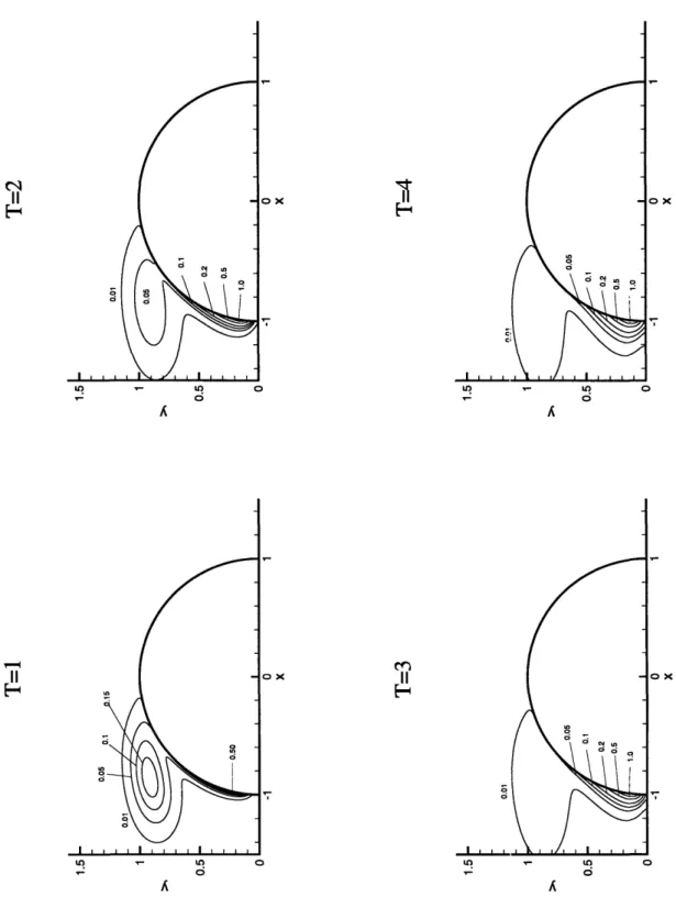
where x~' r= cos 0, y = r' sin 0. In all calculations we take r' =: 1.3 and S = 0.1. The Coriolis factor is taken to be f = 0.8. Three locations of initial releases have

been considered: Oc = 45', Oc = 90', and f, = 135'. In each case the snapshots at

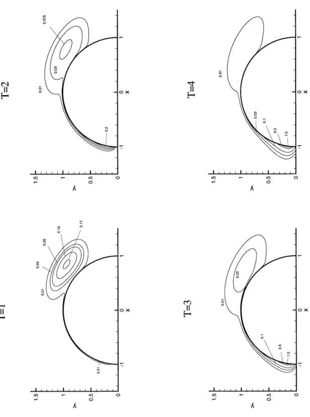
T' = 1, T' = 2, T' = 3, and T' = 4 are plotted. Note that for ro = 50 km, U = 1 m/s, w = 1.45 x 10- 4 _{1/s), T =' 1 corresponds to 4.2 days. For comparison the tidal time}

scale is 1/w = 0.08day. In figures I-4-1 we show the concentration contours when the

initital cloud center is at r' = 1.3, 0 = 450. At T' = 1 the initially concentric circular contours become tilted ellipses due mainly to the off-diagonal dispersivities (Exy and

Ey). Some particles are transported toward the coastline around the point (r' = 1,

0 = 45') as a result of both Eulerian convection and diffusion from the cloud center.

Since the normal flux vanishes at the vertical shore, particles tend t;o pile against the shore and the local radial gradient of the concentration reverses, i.e., DC/Or changes from positive to negative. Consequently, two local concentration peaks appear, one, designated as P₁, say, corresponds to the center of the initial cloucd which is affected

II OX ox Hd I I I l Il l I t -- _A o =- _A 0 6 III l lt tx

Figure I-4-1: Evolution of particle concentration. Cloud center is initially released at north-east (r' = 1.3,

0c

mainly by convection, since the local concentration gradient is zero. The other peak corrresponds to the accumulation along the coast, designated as P2, say, and moves along the circular coastline. Note that at T' = 1, P1 has not moved much from its

original location owing to the small local convection velocity (cf. figure I-4-1.a). P2, however, is displaced quite far from the where the particle cloud first reaches the coast. More interesting is that P2 passes the point where the Eulerian streaming converges around (r' = 1, 9 = 1350), instead of stopping there. To understand this phenomenon we express in polar form:the component of particle flux along the circular coastline,

0C

Fo = UoC - Er Or r (1.4.2)

Or r 19

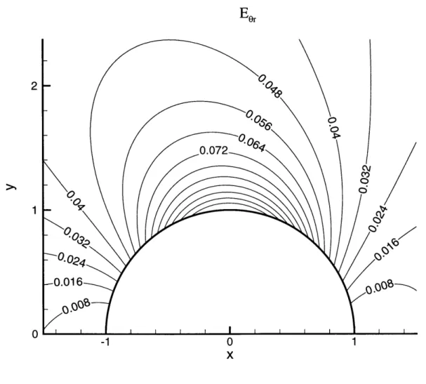
The last term plays a small role in displacement of P2 where C/09 vanishes. The second term on the right-hand side stands for the longshore flux due to the radial gradient, a result of the off-diagonal dispersivity, Eor. As shown in figure 1-4-2, Eor

is positive along the entire rim of the island.

Since 0C/Or is negative, the longshore flux is along the positive 0 direction. Now the physical picture is clear:

i) When a peak is formed at the coastline due to local accumulation of particles, it is transported along the direction of increasing 0 by both convection and diffusion; ii) When the peak of accumulation P2 reaches the converging point of the convec-tion field, the term representing off-diagonal dispersibity Ear OC/Or dominates and

tends to move the peak P2 past the point of velocity convergence. The clockwise convection velocity is too weak to counter the trend until the peak finally is stopped by the straight coastline.

From Figure I-4-1 b-d it can be seen that P moves from its original location (0.9,0.9) in x, y plane to about (0.8,1.0). The concentration at P2 increases with time

due to additional accumulation of particles.

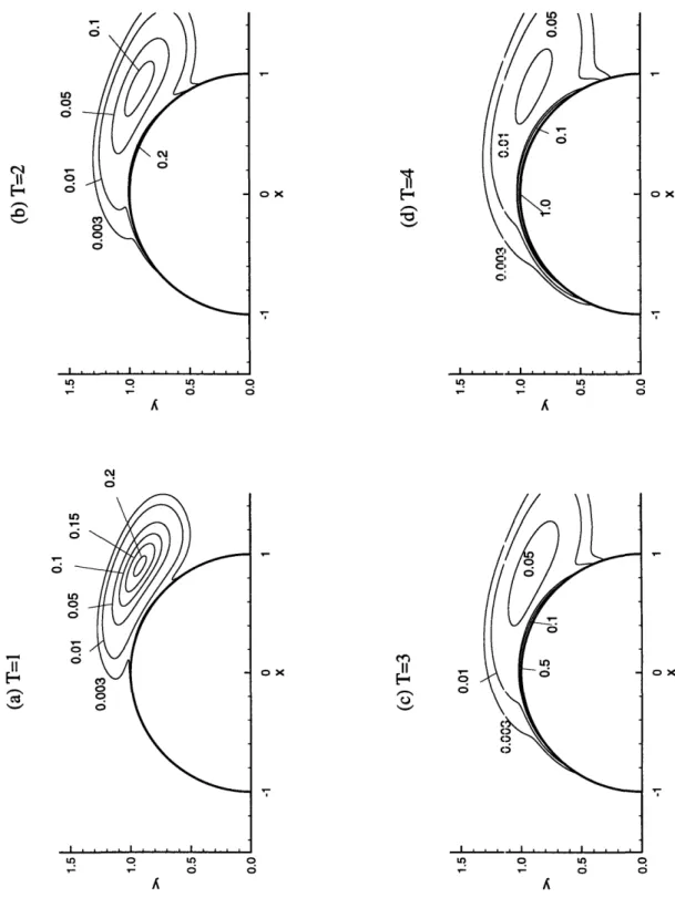
For other locations of initial release, the results are qualitatively the same (see Figure I-4-3 a-d for initial release at (r' = 1.3, 9C = 1350)).

concen-1- -g \ I II/ " ' \ I ! C" 0.024 0.016 _Oso 0 -1 0 1 X

Figure 1-4-2: Off-diagonal dispersivity tensor component Ee, around a circular

(I x itox 0 X d , ,- . H H Cc-00 II ox II -l x ~ ~oo m~~~ om r , u o o I n '- In 0 I ,= In 0 d d A A

Figure 1-4-3: Evolution of particle concentration. Cloud center is initially released at

tration cloud eventually reaches and stays around the stagnation point at r' = 1, = 180.

Along the equator the effects of earth rotation vanish since f = 0; the velocity field is symmetrical with respect to the y axis. Accordingly, the convection field and the dispersivity tensor are symmetrical with respect to the y axis. No matter where it is initially released, the cloud finally moves to the coastline and converges to the offshore tip of the peninsula. We only show in figure I-4-4 the results for the case

where the center is released at r' = 1.3, 0 = 450.

Thus convection by Eulerian streaming, already predicted by Larmoure and Mei (1977), dominates the phenomenon, unlike the case with f 7 0.

As a confirmation of numerical accuracy, we check that total mass is conserved in the non-erosion case:

M = Mo= C(x,y)dxdy = C(r, O)rdrdO

= JC((, ?)e2r|J ddr, (1.4.3)

where the Jacobi determinant is given by

S

(

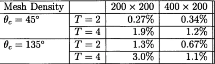
With time marching, the computed total mass however, increases slightly due mainly to the temporal accumulation of numerical errors and the inaccuracy in numerical integration for the total mass. The improvement of numerical accuracy by denser grids is shown in the following table where the relative mass increase is shown at a certain time after an initial release at a particular location.

u, o u o 0 0 q 0 A ox 0 0 A CI II H Yid H So r o 0 0

Figure 1-4-4: Evolution of particle concentration. Cloud center is initially released at north-east (r = 1.3, Oc = 450) for f = 0, Pe = 1 and Sc = 1.

ox

ox

Mesh Density 200 x 200 400 x 200

0c = 450 T = 2 0.27% 0.34%

T = 4 1.9% 1.2%

Oc = 135o T =2 1.3% 0.67%

T = 4 3.0% 1.1%