This is an author-deposited version published in :
http://oatao.univ-toulouse.fr/
Eprints ID : 8796
To link to this article : DOI:
10.1103/PhysRevE.87.012718
URL :
http://dx.doi.org/10.1103/PhysRevE.87.012718
O
pen
A
rchive
T
OULOUSE
A
rchive
O
uverte (
OATAO
)
OATAO is an open access repository that collects the work of Toulouse researchers and
makes it freely available over the web where possible.
To cite this version :
Davit, Yohan and Byrne, Helen and Osborne, James and
Pitt-Francis, Joe and Gavaghan, David and Quintard, Michel
Hydrodynamic dispersion within porous biofilms.
(2013) Physical
Review E, vol. 87 (n° 1). pp. 1-16. ISSN 1539-3755
Any correspondence concerning this service should be sent to the repository
administrator:
[email protected]
Hydrodynamic dispersion within porous biofilms
Y. Davit,1,2,3H. Byrne,1,4J. Osborne,4J. Pitt-Francis,4D. Gavaghan,4and M. Quintard2,3 1Mathematical Institute, University of Oxford, 24-29 St Giles’, Oxford OX1 3LB, United Kingdom 2Universit´e de Toulouse; INPT, UPS; Institut de M´ecanique des Fluides de Toulouse (IMFT), All´ee Camille Soula,
F-31400 Toulouse, France
3CNRS IMFT, F-31400 Toulouse, France
4Department of Computer Science, Oxford University, Wolfson Building, Parks Road, Oxford OX1 3QD, United Kingdom
Many microorganisms live within surface-associated consortia, termed biofilms, that can form intricate porous structures interspersed with a network of fluid channels. In such systems, transport phenomena, including flow and advection, regulate various aspects of cell behavior by controlling nutrient supply, evacuation of waste products, and permeation of antimicrobial agents. This study presents multiscale analysis of solute transport in these porous biofilms. We start our analysis with a channel-scale description of mass transport and use the method of volume averaging to derive a set of homogenized equations at the biofilm-scale in the case where the width of the channels is significantly smaller than the thickness of the biofilm. We show that solute transport may be described via two coupled partial differential equations or telegrapher’s equations for the averaged concentrations. These models are particularly relevant for chemicals, such as some antimicrobial agents, that penetrate cell clusters very slowly. In most cases, especially for nutrients, solute penetration is faster, and transport can be described via an advection-dispersion equation. In this simpler case, the effective diffusion is characterized by a second-order tensor whose components depend on (1) the topology of the channels’ network; (2) the solute’s diffusion coefficients in the fluid and the cell clusters; (3) hydrodynamic dispersion effects; and (4) an additional dispersion term intrinsic to the two-phase configuration. Although solute transport in biofilms is commonly thought to be diffusion dominated, this analysis shows that hydrodynamic dispersion effects may significantly contribute to transport.
I. INTRODUCTION
Biofilms are sessile communities of microbes that develop on solid or liquid interfaces, embedded within extracellu-lar polymeric substances (EPS) [1]. These aggregations of microorganisms represent the dominant form of microbial life on Earth and have considerable sanitary, ecological, and economic impact. Effects can be desirable (wastewa-ter processes, bioremediation, industrial and drinking wa(wastewa-ter treatment, sequestration of carbon dioxide) or undesirable (paper manufacture, microbially influenced corrosion within pipelines, heat exchangers, or on ships) and, potentially, harmful (contamination in the food industry, disease, chronic infections, sustainability of water supply networks). Within the last few decades, understanding and controlling biofilm growth have emerged as major scientific challenges. An important component of these challenges is to understand how chemicals and particles are transported within biofilms, in order to (1) elucidate their resistance to antimicrobial agents; (2) design efficient control and staining strategies; (3) develop reliable growth models; and (4) describe the exchange of signaling molecules or genetic material between cells. These transport phenomena generally result from coupled biological, physical, and chemical processes occurring over a large spectrum of temporal and spatial scales.
In the early days of biofilm research, mathematical and con-ceptual models treated these consortia of microorganisms as a homogeneous coating of a solid surface. Later on, experiments showed that biofilms can form intricate architectures with pores, voids, and channels. For example, Stoodley et al. [2] used confocal laser scanning microscopy (CLSM) to perform
particle image velocimetry (PIV) analysis and map the velocity field within biofilms grown under different conditions. They reported fluid flow inside biofilm channels and observed situa-tions in which water flowed against the main current of the bulk water phase. Massol-Dey´a et al. [3] used CLSM and scanning electron microscopy to observe multispecies aerobic biofilms growing in a granular activated-carbon fluidized-bed reactor. They describe channel-like and coral-reef structures. Hidalgo
et al.[4] used CLSM to obtain tomographic pH images of highly heterogeneous biofilms. Advances in optical coherence tomography (OCT) also suggest complicated geometries. Wagner et al. [5] analyzed the structure of heterotrophic biofilms on relatively large volumes using OCT and revealed an incredible level of complexity.
Wimpenny et al. [6,7] and Loosdrecht et al. [8] suggest that these heterogeneities may result from a combination of factors including shear stress, diffusion limitations, and substrate concentration. Davey et al. [9] showed that the architecture of Pseudomonas aeruginosa biofilms is actively regulated by the production of rhamnolipid surfactants. Houry
et al.[10] show that planktonic bacteria propelled by flagella can create large transient pores in the cell cluster and suggest that swimmers “may improve biofilm bacterial fitness by increasing nutrient flow in the matrix.” It has also emerged— for example, see discussions by Plalkov`a et al. [11]—that wild strains in real environments tend to form more heterogeneous structures than laboratory strains. These results have led to the idea that biofilms are complex structures, rather than dense impermeable gel-like layers. These studies have also identified two classes of channels, as discussed in Ref. [6] and illustrated
FIG. 1. (Color online) Examples of heterogeneous biofilms and fluid channels. (a) Top view of a polymicrobic biofilm grown on stainless steel where water channels have formed between the cell clusters (public domain, reproduced from Ref. [13]). (b) Cross-sectional view of intracluster channels obtained using optical coherence tomography (reproduced, with permission, from Ref. [5]). (c) Top view of a Bacillus thuringiensis biofilm where the arrow indicates a transient channel created by swimmers (reproduced from Ref. [10]).
in Fig.1(see also images in Ref. [4] and [12]): intracluster channels that may result from mechanical interactions with the fluid phase, fracturing of cell clusters, predation, or swimmers; and extra-cluster channels that form between cell clusters. We remark that most studies have focused on biofilms grown on flat surfaces and that the intra- versus extra-cluster distinction may be inappropriate for biofilms grown on more intricate substrata. In the remainder of this work, we will use the generic
terminology “channel” to specify passages (over a range of sizes and from different origins) through which fluids may flow and “porous biofilms” to describe heterogeneous biofilms involving channels, voids, or pores.
The realization that biofilms can form intricate porous systems has led to the emergence of models which include fluid flow. For example, Dupin et al. [14] and Thullner and Baveye [15] determined the velocity field within the bulk fluid phase, viscosity µf, and within the biofilm by considering a
fictitious weighted viscosity within the biofilm phase, µb=
γ µf with γ > 1. Kapellos et al. [16] developed a simulator
that couples a cellular automaton with multiscale methods. They used a single-domain volume-averaged formulation, originally developed for Darcy-scale fluid-porous interfaces (see in Ref. [17]), to model the fluid flow within the bulk fluid and biofilm phases. Surprisingly, these studies have focused on momentum transport, and have not addressed the effects of biofilm permeability on mass transport. Within these structures, transfer of a molecule, or a particle, is influenced by a number of mechanisms, including advection, which may significantly impact the transport properties of important chemical species, such as nutrients or antimicrobial agents. Models should carefully incorporate these mechanisms into the mathematical description of biofilms.
Solute transport in biofilms, regardless of their architecture, is often characterized by the ratio De/Daq, of the effective
diffusion coefficient De and reference (culture medium or
growth fluid) diffusion coefficient Daq. Various experimental
techniques have been used to calculate the effective diffusion
coefficient; a review of these techniques can be found in Ref. [18] and further discussions are available in Refs. [19,20]. For the purposes of this paper, we outline the main exper-imental devices that have been used to measure effective diffusion coefficients, including recent developments. Bungay
et al.[21] used the oxygen microelectrode technique, while Matson and Characklis [22] used a two-chamber method to measure oxygen and glucose diffusion coefficients in sludge flocs. de Beer et al. [23] used a combination of oxygen microelectrode measurements and CLSM to correlate concentration gradients with the structure of aerobic biofilms. Lawrence et al. [24] observed the diffusion of fluorescein and fluor-conjugated dextran in Pseudomonas fluorescens using fluorescence recovery after photobleaching (FRAP) and CLSM. Bishop et al. [25] calculated the effective diffusion coefficient from the structure of frozen 10–20-µm slices of biofilm. Stewart et al. [26] measured the diffusion coefficient of tagged daptomycin in cells clusters of Staphylococcus
epidermisusing CLSM. Recently, methods involving nuclear magnetic resonance (NMR) were proposed to obtain effective diffusion coefficients in situ [27,28]. Advances in x-ray microtomography also offer new perspectives for studying in
situtransport properties in porous structures [29,30] and for estimating the corresponding diffusion coefficients.
Although Daq is well defined for a given temperature,
solute, and growth medium, the interpretation of De is
ambiguous. Active biological processes, such as uptake rates, or physicochemical properties of the biofilm, the solute, and the bulk fluid phase, are difficult to correlate with De. Many
studies have focused on identifying those parameters that most strongly influence De. Several authors have proposed
empirical relationships between De/Daq and the biofilm
density ρ for passive transport [31]. Hinson and Kocher [32] used the fraction of EPS as an additional parameter. Stewart [18] investigated the influence of chemical properties on De/Daq, such as the charge of the EPS or the molecular weight
of the solute molecules. These correlations could be extended in many ways to account for other biochemical processes. Such formulas are extremely important because they can be widely used by experimentalists. However, many fundamental aspects of solute transport are still a matter of debate [33]. For example, the following points have received little attention from a mathematical modeling point of view. Biofilms are known to form heterogeneous structures (see [34]), with spatially and dynamically varying diffusion coefficients. This raises several fundamental questions, such as: How does such heterogeneity influence De? Is it valid to use a single effective value of the
diffusion coefficient, or should a spatially resolved coefficient be used? With regard to advection within biofilms, is it possible to characterize solute transport in terms of the ratio De/Daq
when there is fluid flowing within the biofilm? Is it even possible to define effective diffusion coefficients in this case? With regard to reaction, do uptake rates and degradation of the solute influence the ratio De/Daq or do they only affect the
effective reaction rate?
In addition to the above theoretical issues, there is often ambiguity in the interpretation of experimental estimates for De. Recently, Wagner et al. [5] emphasized this problem by
comparing estimates of biofilm porosities obtained using OCT and CLSM. For a Reynolds number of 4000 in the bulk fluid
phase, the porosity of the biofilm was found to be about 0.98 using CLSM and 0.35 using OCT. The authors suggest that OCT provides a more reliable framework for studying biofilm structures because it does not require fluorescence staining, and therefore does not rely on the transport properties of the biofilm, and is not limited by laser penetration depth. This is an important observation because CLSM is widely used to measure structural biofilm properties, and this may lead to erroneous conclusions. These results have wider implications that go beyond the issue of CLSM applicability: they suggest that caution should be exercised when interpreting experimental data for biofilms.
All the techniques discussed above differ in terms of their physical significance, and parameters, such as De, should
be defined in relation to a specific experiment. Particularly relevant to this discussion is the spatial resolution of the experimental method under consideration. For example, the NMR technique used in Ref. [28] has an in-plane resolution of 7.5 × 250 µm, whereas x-ray microtomography and/or OCT can resolve to several micrometers. CLSM can achieve a similar resolution, but this is strongly dependent on the fluo-rescent staining. Two-chamber experiments only capture bulk information within each chamber. The parameters that are measured using these techniques are averaged over different volumes, and their physical interpretation is different. For example, if the biofilm contains fluid channels of approximate width 10 µm, then a technique with a resolution of 100 µm is measuring a concentration field and/or a diffusion coefficient averaged over both the cell clusters and the channels. On the other hand, a technique with a resolution of several microm-eters can delineate between the two and/or provide a local diffusion coefficient for layered cell clusters. Experimental studies should carefully address these issues.
Upscaling techniques, such as volume averaging with closure (see [35]), can be used rigorously to define the ratio De/Daqand, therefore, to address the above theoretical
and experimental issues. With such techniques, averaged equations at the biofilm scale can be obtained from transport equations at the channel and cellular scales, provided that
several spatial and temporal scale constraints are satisfied. An important feature of this approach is that the set of homogenized partial differential equations contains effective coefficients that can be directly related to the topology of the problem at the microscale, thereby allowing physical understanding of the contribution of the different processes. In addition, these methods may be used to develop novel ways of measuring effective diffusion coefficients. In particular, real geometries and velocity fields obtained via imaging techniques, e.g., tomography, may be directly used for the computation of effective coefficients. This strategy is an alternative to the standard inverse optimization method where effective coefficients are determined by optimization of model parameters using biofilm-scale data. A clear advantage of the upscaling method when compared with inverse optimization is that the effective parameters and the scale constraints are unambiguously defined. A disadvantage of this approach is that the experimental techniques that capture the information necessary for such calculations are new and the complete imaging-upscaling strategy has not yet been fully applied to real systems.
Even so, there is another advantage to homogenization techniques that does not require accurate knowledge of real geometries: it yields the domains of validity of the models. The mathematical procedure of homogenization generally involves order of magnitude estimates which apply to dimensionless numbers. For instance, in the case of Taylor dispersion, one usually requires that the P´eclet number is such that the time for a molecule to diffuse radially is much smaller than the time for longitudinal transport. In addition, the averaging procedure, as presented in this paper, applies to an ensemble of geometries that is defined by length scale constraints. Therefore, models are not limited to a given geometry, but to a class of geometries, and the domains of validity apply to this entire class. Similarly, dimensionless numbers can be used to study important features of the models on simplified systems. For example, we can readily answer one of the questions presented above: Do uptake rates and degradation of the solute influence the ratio De/Daq
or do they only affect the effective reaction rate? In Refs. [36] and [37], it is shown using two-dimensional unit cells that the longitudinal dispersion coefficient decreases with the Damk¨ohler number, Da, or equivalently the Thiele modulus, when Da& 10. The quantitative behavior will change with the geometry but not the order of magnitude estimate. This is important because it means that for, say, Da6 1, we can consider that the effective diffusion is the same for the reactive and nonreactive cases. Unfortunately, there is little experimental data that can be used to estimate Da, essentially because its estimation requires knowledge of the diffusion coefficient, the form of the reaction rate, and the values of the reaction parameters. Stewart and Raquepas [38] calculated the Thiele modulus for reactive antimicrobial agents and found values in the range 0.44–18.2, suggesting that both situations may be encountered.
In this work, we will focus on the nonreactive case and use the volume averaging method to study some physical aspects of solute dispersion within porous biofilms. As discussed above, the analysis also applies to the reactive case when the dispersion coefficients do not depend upon uptake rates, i.e., when Da6 1. Similar developments were presented in Refs. [35,39,40], but these papers focused on upscaling solute transport from the cellular to the cell cluster scale. The effect of advection within channels was studied in Ref. [40] but only in the limiting case where spatial gradients at the microscale are negligible, a situation termed local mass equilibrium. Here, we do not assume local mass equilibrium and show that relaxing this assumption leads to significant changes to the macroscale equations. Our modeling framework requires that biofilms should not be defined as cell clusters alone, but as a two-phase mixture of a cell cluster phase (ω) interspersed with a fluid-flow-channel phase (κ). We use a multiscale strategy to derive an effective diffusion tensor for this situation. Within the cell-EPS matrix (i.e., the cell clusters) the solute is transported by diffusion alone, but the diffusion coefficient can vary “arbitrarily” (although smoothly) in space. In the channels, the solute is transported by advection and diffusion.
Our primary goal is to answer the following questions: (1) Are hydrodynamic dispersion effects significant within porous biofilms?
(2) Can we define an effective diffusion which describes fluid flow within the channels and spatially varying diffusion
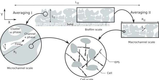
FIG. 2. Schematic diagram highlighting the multiscale nature of biofilms. Two different ways of averaging are presented depending on the scale constraints that are satisfied: on the left, the averaging volume is defined on a small portion of the biofilm; this is appropriate if the average diffusion coefficient within the cell clusters varies slowly throughout the biofilm and if channels are relatively small (i.e., RI≪ LI); on the
right, the averaging volume is defined over the entire height of the biofilm, with a diffusion coefficient within the cell clusters which varies with depth and macrochannels (i.e., only RII≪ LII). Three spatial scales can be identified: the biofilm scale, the channel scale, and the cell scale.
Each region illustrates a representative elementary volume of the corresponding larger scale. We remark that, for averaging II, the macroscale concentration fields within the biofilm will only vary along the X direction and boundary conditions should be treated carefully. In this work, we will focus primarily on upscaling from the channel scale to the biofilm scale with averaging I and defer averaging II to future work.
coefficients within the cell clusters? What are the physical processes corresponding to these effective dispersion coeffi-cients?
(3) Should we always use the effective diffusion model to describe solute transport within porous biofilms? What are the alternatives?
The remainder of this study is organized as follows. In Sec. II, we briefly review experimental evidence for hydrodynamic dispersion within porous biofilms. In Sec.III, we detail our microscale problem. A representative elementary volume (REV) of the system is presented in Fig. 2 and the corresponding mathematical model at the channel scale is presented in Sec.III. We are interested in hierarchical systems for which lκ ≪ R ≪ L, where lκ is a characteristic width
of the channels, R is the radius of the REV, and L is a characteristic macroscale length for the biofilm. In Sec.IV, we perform a perturbation analysis, termed the volume averaging with closure technique, to derive the macroscale models. For brevity, the key results are presented in the main text, while technical details are provided in the Appendix or in specific references. In Sec. VII, we discuss potential applications of these models, their limitations, and future work. In Sec.VIII, we summarize the main modeling results and the answers to the above questions.
II. EXPERIMENTAL EVIDENCE OF HYDRODYNAMIC DISPERSION EFFECTS IN BIOFILMS
It is now commonly accepted that channels are an essential part of biofilms (see [20]) and that advection effects are integral to solute transport within such systems. Even so,
the channels and cell clusters are traditionally treated as two distinct phases. In Ref. [19], when discussing the issue of diffusion limitation inside cell clusters, Stewart states that “structural heterogeneity in a biofilm changes the geometry of the diffusion problem, but it does not alter the fundamental phenomena.” Our goal in this section is to challenge this view. We argue that, while the microscale balance equations rely on advective and diffusive transport models, the fundamental phenomena captured by the notion of effective diffusion depend on both the scale of observation and the structural
heterogeneities. Indeed, the homogenization of a problem with diffusion and advection at the microscale will produce a continuum representation in which the phase delineation has disappeared but in which the effective parameters depend on the heterogeneities. For example, effective dispersive fluxes will contain hydrodynamic dispersion effects that originate from fluctuations in the velocity field and tortuosity effects that describe the geometry of the microstructure. Similarly, within porous biofilms, we anticipate that there will be hydrodynamic dispersion effects produced by fluctuations in the velocity fields and tortuosity effects that will reflect the topology of the channel network within the biofilm. In this section, we provide experimental evidence that hydrodynamic dispersion may indeed occur. Our demonstration is based on the following two classes of experiments: (1) biofilm-scale measurements of effective diffusion that have reported De/Daq>1; and
(2) channel-scale measurements of the velocity field within a biofilm which suggest that advection effects may be important. We start with biofilm-scale measurements and focus on studies that have reported peculiarities in the ratio De/Daq. In
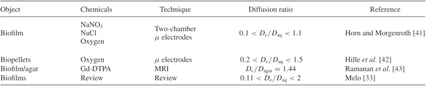
TABLE I. Examples of studies in which the effects of dispersion and advection have been observed in biofilms and biopellets.
Object Chemicals Technique Diffusion ratio Reference
NaNO3 Two-chamber
Biofilm NaCl 0.1 < De/Daq<1.1 Horn and Morgenroth [41]
µelectrodes Oxygen
Biopellets Oxygen µelectrodes 0.2 < De/Daq<1.5 Hille et al. [42]
Biofilm/agar Gd-DTPA MRI De/Dagar= 1.44 Ramanan et al. [43]
Biofilms Review Review 0.11 < De/Daq<2 Melo [33]
Ref. [19]). In these situations, the path of a solute molecule in a cell cluster is constrained by the presence of obstacles (cells, extracellular polymeric substances, abiotic particles) and a notion of tortuosity can be invoked [33]. Interestingly, in some low-density biofilms and in fungal biopellets, this ratio has also been reported to be larger than unity (cf. TableI). Melo [33] argues that the tortuosity, 3, defined by De= Daq/3, can be
lower than unity if the solute undergoes convection inside the biofilm. This is an interesting idea, but it also suggests that a lot of physics is hidden within Deand that a notion of tortuosity
alone might not be sufficient. Hydrodynamic dispersion can be used to interpret these results if the P´eclet number, Pe = Dυdaq, where υ is an average velocity and d a characteristic length, is sufficiently large. In the case of the biopellets, the flow is not limited by the EPS, and even larger ratios, De/Daq>1, have
been reported when the cell density is relatively low (e.g., in Ref. [42], Fig.3, p. 1207).
Even when De/Daq<1, it is not straightforward to
determine the relative contributions of diffusion and advection to solute transport. It is commonly accepted that De/Daq<1
corresponds to a diffusion-dominated transport. For instance, Horn and Morgenroth [41] clearly state that “[...] convective transport would have resulted in De/Daq>1. The results
presented indicate that for biofilms older than a few days and with mean biofilm density higher than 20 kg/m3 convective
transport can be neglected.” We question this interpretation. In the case of porous biofilms, De/Daq<1 means that the
combined effects of the advective and diffusive “components” (a clear definition of these components is given later in this paper) leads to a reduction in the diffusion coefficient, but this does not mean that the advective component is negligible compared to the diffusive one. A ratio smaller than unity, say De/Daq= 0.9, may very well mean that Dediffusion/Daq= 0.2
without advection effects. For example, if hydrodynamic dispersion occurs within the channels, then the transition from De/Daq<1 to De/Daq> 1 is continuous, and there is a region
of parameter space for which De/Daq<1 is compatible with
hydrodynamic dispersion. For example, Ramanan et al. [43] estimated the diffusion coefficient of a complex of gadolinium and diethylenetriamine pentaacetic acid (Gd-DTPA) using magnetic resonance imaging with an in-plane resolution of 150 µm × 150 µm. They observed the concentration fields in agar, a highly permeable gel, and in a phototrophic biofilm. The diffusion coefficient in the biofilm was found to be larger than that in the highly permeable gel. Using this comparison, the authors deduced that transport in the biofilm,
¯
x
(10−5m) Increasing t ↓ C o n ce n tr a ti o n ¤ c ωκasy − c ωκ tel¯
x
(10−5 m)t
(s) 0 2 4 6 8 10 0 10 −10 0 0.1 0.2 0.3 0.4 0.5c
ωκasyc
ωκtel(a) Analytical solutions, c ωκasy and cωκtel (b) Difference, c ωκasy c ωκ
tel
FIG. 3. (Color online) Illustrations of the telegrapher’s and advection-dispersion fundamental solutions for hciωκ( ¯
x,t = 0) = δ( ¯x), ∂thciωκ( ¯x,t = 0) = 0, T = 1 s, and De= 10−10m2s−1: (a) Plot of hciωκtel (Telegraph), Eq.(26), and hciωκasy(Gaussian), Eq.(27). Each curve
represents the solution at a given time. Notice that the front, in the telegrapher’s solution, involves a Dirac distribution. (b) Plot showing how the difference hciωκ
asy− hci ωκ
tel between the fundamental solutions evolves over time. The telegrapher’s equation can be interpreted as an
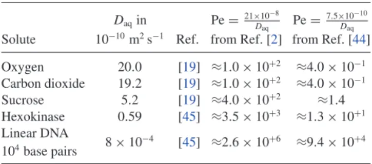
TABLE II. Diffusion coefficients in pure water at 25◦C and
corresponding P´eclet numbers for example solutes. Daqin Pe =21×10
−8
Daq Pe =
7.5×10⁻¹⁰
Daq
Solute 10−10m2s−1 Ref. from Ref. [2] from Ref. [44]
Oxygen 20.0 [19] ≈1.0 × 10+2 ≈4.0 × 10⁻¹ Carbon dioxide 19.2 [19] ≈1.0 × 10+2 ≈4.0 × 10⁻¹ Sucrose 5.2 [19] ≈4.0 × 10+2 ≈1.4 Hexokinase 0.59 [45] ≈3.5 × 10+3 ≈1.3 × 10+1 Linear DNA 8 × 10⁻⁴ [45] ≈2.6 × 10+6 ≈9.4 × 10+4 104base pairs
although they observed De/Daq<1, was by both diffusion and
advection.
The second part of our argument relies on direct ex-perimental confirmation that the P´eclet number within the fluid channels may lie in the range that yields hydrodynamic dispersion effects. Our calculations of the P´eclet numbers are based on average velocities, calculated using PIV measure-ments performed in Refs. [2] and [44]. We remark that these correspond to extra-cluster channels for biofilms grown on flat surfaces and, to the best of our knowledge, experimental data for intracluster velocities or biofilms grown on more complex substrata (e.g., in porous media) do not yet exist. Figure5in Ref. [2] supplies an average velocity of ≈ 3 × 10⁻³ m/s for a characteristic length of ≈ 70 µm; and Fig. 5in Ref. [44] indicates a velocity of ≈ 1.5 × 10⁻⁵ m/s for a characteristic
length of ≈ 50 µm. Using these values, we can calculate the P´eclet number associated with the transport of various chemicals for a temperature of 25◦C. The results presented
in Table II show that the P´eclet number may take large values, especially for macromolecules. The results for large linear DNA macromolecules are presented to illustrate the limit Daq→ 0 and to show that a large P´eclet number does
not necessarily correspond to large hydrodynamic forces. For Pe& 1–10, fluctuations in the velocity field within the fluid channels will induce hydrodynamic dispersion effects. We remark that the reference diffusion coefficient should correspond to the solvent in the water channels, rather than pure water, and that Daq in Table II is therefore an upper
bound for the reference diffusion coefficients. Consequently, the values of the P´eclet numbers presented in TableIIshould be viewed as lower bounds.
III. MICROSCALE MODELING FORMULATION
As discussed previously, the biofilm can be decomposed into two distinct phases: a cell-EPS matrix phase (ω) and the fluid-channels phase (κ) (see Fig.2). Within the cell-EPS matrix phase, the solute is transported by diffusion alone but the diffusion coefficient can vary in space. In the channel phase, the solute is transported by diffusion and advection. Delineating explicitly between the bulk water phase and the channels is an important problem that should be carefully addressed in the future. However, for the purposes of this study, we consider an idealized channel phase and suppose that all interfaces are static. This assumption is valid if the time scales associated with the transport phenomena and the growth processes are markedly different (e.g., in Ref. [46]),
and can be further justified by the stated aim to understand mass transport itself, rather than its coupling with growth.
By considering conservation of mass for a given solute, the following system of equations can be used to describe transport in this system: ∂cω ∂t = ∇ · [Dω(r)∇cω] in Vω, (1) nωκ· [Dω(r)∇cω] = nωκ· (Dκ∇cκ) on Aωκ, (2) cω= cκ on Aωκ, (3) ∂cκ ∂t + ∇ · (vκcκ) = ∇ · (Dκ∇cκ) in Vκ. (4) In these equations, cα is the pointwise concentration
(nutrient or antimicrobial agent) in the phase (α) with (α = ω,κ); Dω(r), also referred to as Dω for simplicity, is
the diffusion coefficient within the cell-EPS phase (it may vary with spatial position); Dκ is the diffusion coefficient in
the channel phase; Vαis the open bounded set that represents
the α phase within the REV; Aωκis the interface between the
channel phase and the cell-EPS phase; nωκ is the unit vector
normal to Aωκ pointing from ω to κ; and vκ is the velocity
field in the fluid phase. We will suppose that the velocity field is known pointwise throughout the entire system, in order to focus on mass, rather than momentum, transport (the reader is referred to Ref. [47] for an extensive discussion on fluid flow in biological media). We will also assume that Dωcan be
actively modified by the microorganismsbut that its average value over a REV varies slowly throughout the biofilm.
For simplicity, we will only use averaging I in Fig. 2, with an extension to averaging II that would involve similar models but that requires one to consider the solid and the biofilm–bulk-fluid boundaries. We remark that averaging II will produce macroscale models for the biofilm with reduced dimensionality, i.e., a three-dimensional biofilm will be treated as a two-dimensional (2D) interface. This idea is reminiscent of the notion of an effective boundary condition that was discussed by Veran et al. [48] in the case of rough reactive walls. We will explore this idea further in future work. In addition, we emphasize that this distinction only represents a schematic view of the problem and that, from a theoretical point of view, the only relevant criterion is the separation of length scales, i.e., we require R ≪ L.
In Eq.(2), we have assumed that the velocity field vanishes on Aωκ so that the interfacial flux across the boundary is
purely diffusive. We have further assumed that the system is at thermodynamic equilibrium, and that equality of the chemical potentials on Aωκ leads to continuity of the concentrations
there. In practice, this purely thermodynamic constraint could be easily relaxed by applying a suitable constitutive law for the chemical potentials. For instance, in diluted cases, this equality is often written in terms of a jump condition for the concentrations, cω= Kcκon Aωκ, in which K is a function
of the pressure and the temperature. For the purposes of the upscaling performed in the remainder of this study, the only constraint that is mandatory is that this relationship between cω
and cκshould be affine. For simplicity, we restrict attention to
on Aωκ would be straightforward, using a simple change of
variables.
IV. MULTISCALE PERTURBATION ANALYSIS
In this section, the transport equation in each phase is averaged in space (as defined in Fig.2), and the pointwise fields are decomposed into an averaged part plus a perturbation. The averaged component is allowed to vary on a characteristic length scale R within a macroscopic domain of length L, while the perturbation varies with a characteristic length lκ, where
we assume L ≫ R ≫ lκ in order to perform an asymptotic
analysis.
A. Definitions
First, we define the volume of the phase (α = ω,κ), Vα=
R
VαdV, and the total volume of the REV, V = Vω+ Vκ.
We denote the superficial average of any tensor field πα(for
tensors of order 0, 1, or 2) by hπαi = V1α
R
VαπαdV. We
define the volume fraction (which we take to be constant throughout the biofilm) of the α phase, εα= VVα, and the
intrinsic average, hπαiα= ε1
αhπαi. We will also use hπi
ωκ
= εωhπωiω+ εκhπκiκ.
We will perform a perturbation analysis by considering decompositions of the form
πα= hπαiα+ ˜πα. (5)
The motivation for this decomposition is that the separation of length scales will impose physical constraints on the perturbation and we will exploit these constraints to make approximations. At this point in the developments, however, it is not possible to determine the validity of these approxima-tions, so that we can only estimate a posteriori the domains of validity of the models. Further, these assumptions, such as the separation of length scales, are not intrinsic to a medium, rather they are process dependent. In other words, for the same biofilm, a homogenized model may be valid for a given value of the flow rate but invalid for a larger one. Equally, it may be valid for a given experimental time scale and not for a shorter one.
The volume average definitions stated above are general in form, and may be used in several ways. Determining the most relevant averaging volume is highly problem specific, depending on the properties of the biofilm and the flow, and on the degree of complexity and precision required.
B. Averaged equations
Transport equations(1) and(4) are averaged in space in the following way to obtain a biofilm-scale description of the system. First, integrals of derivatives are expressed as derivatives of integrals plus surface terms by exploiting general transport and spatial averaging theorems [49]. Secondly, we use the decomposition specified by Eq. (5), along with the assumed separation of scales, lκ≪ R ≪ L, to eliminate
nonlocal terms, i.e., integrals that cannot be calculated locally on the representative volume. Some guidelines are given in Appendix A, and detailed descriptions can be found in Refs. [35,50]. In this way, we arrive at the following system
of macroscopic equations for hcωiωand hcκiκ:
εω ∂hcωiω ∂t − µ 1 V Z Aωκ nωκDωdA ¶ · ∇ hcωiω = εω∇· · hDωiω µ ∇hcωiω+ 1 Vω Z Aωκ nωκ˜cωdA ¶¸ +V1 Z Aωκ nωκ· (Dω∇ ˜cω) dA + εω∇· ˜Dω∇ ˜cω ®ω , (6) εκ ∂hcκiκ ∂t + εκhvκi κ · ∇ hcκiκ = εκ∇· · Dκ µ ∇hcκiκ+ 1 Vκ Z Aωκ nκω˜cκdA ¶¸ + 1 V Z Aωκ nκω· (Dκ∇ ˜cκ) dA − εκ∇· h˜vκ˜cκiκ. (7)
We remark that Eqs.(6)and(7)contain integrals involving correction terms to the average concentrations. To close the problem and obtain a macroscopic formulation for hcαiα
(α = ω,κ), it remains to express these correction terms ˜cα
as a function of hcαiα and its derivatives. This is done in
two steps. First, the boundary-value problem governing the perturbations is derived. A careful analysis in terms of linear differential operators and/or Green’s functions then yields a suitable closure.
C. Perturbations
Since ˜πα = πα− hπαiα, equations for the perturbations
can be obtained by subtracting suitable multiples of Eqs.(6)
and(7) from Eqs.(1)and (4), respectively. In addition, we may neglect derivatives of averaged quantities because, in the continuum limit, the REV can be treated as a “macroscopic point,” i.e., there is a separation of the length scales R ≪ L (cf. detailed discussions in Ref. [35]). In the general case, the fluctuations satisfy a transient problem and the homogenized equations contain time convolutions (e.g., in Ref. [51]). Such a formulation is useful for describing short-time phenomena and accounts for time nonlocality. Since these short-time phenomena are not relevant for our biofilm application, we will consider only a steady-state problem for the fluctuations. This hypothesis is standard and is generally referred to as the quasistationarity of the perturbation problem [35].
The result of this procedure can be written, in the phase (ω), as
(h∇Dωiω− ∇Dω) · ∇ hcωiω
= ∇ · (Dω∇ ˜cω) − h∇ · (Dω∇ ˜cω)iω in Vω. (8)
The boundary conditions are
nωκ· (Dω∇hcωiω− Dκ∇hcκiκ)
= nωκ· (Dκ∇ ˜cκ− Dω∇ ˜cω) on Aωκ (9)
and
hcωiω− hcκiκ = ˜cκ− ˜cω on Aωκ. (10)
In the phase (κ), we have
∇· (vκ˜cκ) − h∇ · (vκ˜cκ)iκ+ ˜vκ· ∇ hcκiκ
Equations(8)–(11)are coupled to Eqs.(4)and(6)and need to be reformulated to facilitate solution. Our goal is to separate the contributions that act on the microscopic level from those that act on the macroscopic level. The first step is to identify the three different macroscopic source terms in these equations: ∇hcωiω, ∇hcκiκ, and hcωiω− hcκiκ. Since Eqs.(8)–(11)are
linear in ˜cαthey can be written as L(˜c) = SV(∇hcωiω,∇hcκiκ),
and B(˜c) = SA(∇hcωiω,∇hcκiκ,hcωiω− hcκiκ), respectively,
in which ˜c = ( ˜cκ,˜cω). L is the linear operator defined in the
bulk phases, B is the linear operator representing the boundary conditions, and SV,SA are the corresponding source terms.
By invoking the superposition principle for this boundary-value problem, the solution can be decomposed into three components, each corresponding to one of the source terms. Again recall that we are interested in the continuum limit R ≪ L, so that these sources can be considered as constant forcing terms and the solution may be written as
˜cα= bακ· ∇ hcκiκ+ bαω· ∇ hcωiω+ sα(hcωiω− hcκiκ) ,
(12) with α = ω or κ.
A different analysis, using Green’s functions (cf. [52]), yields similar expressions for the perturbations. In this case, the solution is also decomposed into components corresponding to the different source terms. The perturbations are then expressed as integrals of the Green’s functions and the source terms, over the spatial variable x′that fixes the position of the
δ. In the continuum limit R ≪ L, we can extract the sources ∇hcωiω, ∇hcκiκ, and hcωiω− hcκiκfrom the integrals and treat
these as constant over the length scale of the REV. Therefore, the mapping variables bαβ and sα can also be interpreted as
integrals of the corresponding Green’s functions over x′. Substituting Eq.(12)into Eqs.(8)–(11)and collecting terms involving ∇hcκiκ, ∇hcωiω, and hcωiω− hcκiκ leads to three
boundary-value problems (given in AppendixB) that govern
bακ, bαω, and sα. These problems are generally solved over a
representative portion of the medium, termed the unit cell, and periodic conditions imposed on the boundary between the unit cell and the rest of the system (note that for averaging II in Fig.2boundary conditions for the top and bottom should be defined carefully). The last step of this procedure is to ensure uniqueness of the solution to Eq.(12), and of the mapping fields. To do this, we fix hbακiα= hbαωiα= 0 and hsαiα= 0
to ensure that h ˜cαiα= 0.
V. CLOSED MACROSCOPIC FORMULATIONS
Now that we have explicit expressions for the perturbations, we return to Eqs.(6)and(7)and obtain a closed form for these macroscopic equations.
A. The two-equation model
Substituting Eq.(12)in Eqs.(6)and(7)leads to εκ∂hc κiκ ∂t + εκ X α=ω,κ ∇· (Vκαhcαiα) = εκ X α=ω,κ ∇· (Dκα· ∇hcβiα) − h(hcκiκ− hcωiω), (13) εω∂hc ωiω ∂t + εω X α=ω,κ ∇· (Vωαhcαiα) = εω X α=ω,κ ∇· (Dωα· ∇hcαiα) − h(hcωiω− hcκiκ). (14)
In Eq.(14), the effective parameters Vαβ, Dαβ, and h can
be expressed explicitly as integrals of the mapping fields over the unit cell. For the velocities, we have
Vαβ = − 1 Vα Z Aωκ nα· {Dα[∇bαβ+ (δαω−δακ)sαI]}dA −V1 α Z Aωκ nα· (Dαδαβ)dA + δαβhvαiα. (15)
For the dispersion tensors, we obtain
Dαβ = hDα[δαβI + ∇bαβ+ (δαω−δακ)sαI]iα
− δαβh˜vαbαβiα. (16)
The mass exchange coefficient is
h = −1 V Z Aωκ nωκ· [Dω(r)∇sω]dA = V1 Z Aωκ nκω· (Dκ∇sκ). (17)
In these equations, we have used δαβ = 1 if α = β and
δαβ = 0 if α 6= β. Here, we have assumed, for simplicity, that
these effective properties are constant through the biofilm, so that Eqs. (13) and (14) can be written in a conservative or nonconservative form.
These upscaling approaches, in which the effective pa-rameters are calculated on a representative portion of the system, are becoming increasingly important given recent advances in imaging techniques such as OCT, CLSM, or x-ray microtomography. Instead of determining only volume fractions, porosities, or densities, we can calculate numerically the effective parameters relevant to a specific application by directly using the images obtained.
Physically, Eqs. (13) and (14) mean that we have a continuous macroscopic transport equation for each phase (dual-continua description), in which mass is exchanged with a characteristic time h−1. Similar models have been used
to describe mass transport in highly heterogeneous porous media [53] and heat transfer problems [54]. Equations(13)
and (14) can be used to describe a broad range of non-Fickian transport phenomena, for which h−1is large compared
to other characteristic time scales associated with transport mechanisms. Such situations may arise when microorganisms actively alter the penetration of the solute or expel it from the cell clusters. We also remark that our model equations are quite general, in that they are not geometry specific, and the phases are arbitrary. For example, upon including the bulk water phase in the definition of the channels and imposing a relevant separation of length scales, our model may be adapted to describe non-Fickian transport phenomena induced by biofilm growth in porous media.
B. Telegrapher’s equations
On neglecting higher order spatial derivatives, it is possible to approximate Eqs. (13) and (14) by a variant of the telegrapher’s equation. This may be written (see AppendixC
for details) · εκεω h ∂2 ∂t2 + ∂ ∂t + Ve· ∇ − ∇ · (D ∗· ∇) ¸ hciωκ +· εκhεω(Vκκ+ Vωω) · ∂ ∂t∇ ¸ hciωκ −½ εκhεω∇· · (Dκκ+ Dωω) · ∂ ∂t∇ ¸¾ hciωκ = 0, (18) where D∗= X α=ω,κ εα(Dαω+ Dακ) − εκεω h [VωωVκκ− VωκVκω] , (19) Ve= X α=ω,κ εα(Vαω+ Vακ) = εκhvκiκ, (20) and hciωκ= εωhcωiω+ εκhcκiκ. (21)
This form of the telegrapher’s equation, Eq.(18), is not standard because it contains mixed time-space derivatives. We can simplify it in the case of an infinite isotropic medium by considering the moving frame ¯r = r − Vetand then neglecting
mixed time-space derivatives. We can obtain the classical telegrapher’s equation (see AppendixCfor details):
εκεω h ∂2 hciωκ ∂t2 + ∂hciωκ ∂t = ∇¯r· (De· ∇¯rhci ωκ) , (22) with De= X α=ω,κ εα(Dαω+ Dακ) −εκhεω[(Vωω− Ve) (Vκκ− Ve) − VωκVκω] . (23)
Equation (22) can be interpreted as a wave equation (∂t t
dominated) with a perturbation (∂t) that disappears at early
times, or as a diffusion equation (∂t dominated) with a
wave perturbation (∂t t) that disappears in the long-time limit
[55,56]. We remark that the wavelike behavior at early times is physically unrealistic for our application because the assumption of quasistationarity of the perturbation problem is not valid in the short-time limit, when nonlocal effects must be considered.
In the mathematical derivation presented in Appendix
C, higher order and mixed space-time derivatives represent a deviation from the classical telegrapher’s model. Higher order terms must be eliminated for consistency with the first-order closure on the perturbations, Eq. (12). However, the influence of the mixed space-time derivatives upon the solutions is not straightforward, and the complete form is given by Eq.(18). Such models, containing mixed derivatives, have been discussed previously in Refs. [57–59] in the case of two-phase heat conduction which are also known as dual-phase-lagging heat conduction models, or in Ref. [59]
for solute contaminant transport. In addition, it is unclear how the standard and nonstandard telegrapher’s equations are related for complex initial and boundary conditions. A further drawback of both telegrapher’s models, as compared to Eqs.(13)and(14), is that an additional initial condition for the time derivative of the averaged concentration is required.
Beyond these difficulties, the similarities between the two-equation and telegrapher’s models are striking and it is tempting to use a telegrapher’s model in a semiheuristic manner to describe non-Fickian solute transport in dual-region media. Future work should therefore focus on understanding the exact mathematical relationship between Eqs.(13),(14),
(18), and(22), for different choices of boundary conditions, initial conditions, parameters and geometries; numerical sim-ulations should be compared with experimental results in order to determine the exact effect of the mixed time-space derivatives.
C. Time-asymptotic behavior
For t ≫ εκhεω, Eqs.(13)and(14)are known, at least in the case of a semi-infinite homogeneous medium, to reduce to a single advection-dispersion equation [60,61]:
∂hciωκ
∂t + Ve· ∇ hci
ωκ
= ∇ · (De· ∇ hciωκ) , (24)
that can also be derived directly from the microscale (see [61]). Heterogeneities or the effects of boundary conditions may trigger a departure from the asymptotic situation, as has been illustrated in Ref. [62]. For the variant of the telegrapher’s model, a similar analysis, e.g., in terms of spatial moments, can be used to show that Eq.(18)has an asymptotic behavior that can be described by Eq.(24). This is straightforward in the moving frame, i.e., by considering the asymptotic behavior of Eq.(22), and then switching back to the static frame.
The dispersion tensor, Eq.(19), can be decomposed into three components by substituting the expressions for Dαβ
(α,β = ω,κ), Eq.(16), into Eq.(23). In this way, we arrive at the following expression for the dispersion tensor (see also [63]): De= X α,β=ω,κ εαhDα(δαβI + ∇bαβ)iα | {z }
Averaged diffusion coefficients and tortuosity
− εκh˜vκ(bκκ+ bκω)iκ | {z } Hydrodynamic dispersion −εωεκ h [(Vωω− Ve)(Vκκ− Ve) − VωκVκω] | {z } Multiphase dispersion . (25)
This expression highlights the notion of effective diffusion that was mentioned in the Introduction of this paper. In addition to terms related to tortuosity and hydrodynamic dispersion, the tensor contains a term specific to the multiphase configuration, which involves Vαβ (α,β = ω,κ) given in
Eqs.(15). This represents a fundamental difference with the expression for the dispersion given in Ref. [40], where the assumption of local mass equilibrium results in the absence of multiphase dispersion. The influence of the hydrodynamic and multiphase dispersion terms depends on the situation. If
there is marked variation in the mean velocities—for example, if the channels have a clear preferred orientation—then the multiphase dispersion term may significantly contribute to the net dispersion effects. However, if the averaged velocity is small—for example, if the channels have no preferred orientation—then the hydrodynamic dispersion originating from velocity fluctuations within the channels will become dominant. We remark further that the effective diffusion is usually characterized by a second-order tensor and can only be described by a scalar when the biofilm is isotropic.
VI. ANALYTICAL AND NUMERICAL RESULTS A. Asymptotic behavior of the telegrapher’s equation
It is important to realize that, although an advection-dispersion equation such as Eq.(24)may seem more familiar than Eqs.(13) and(14) or Eq. (18), there are a number of aspects that make it less pertinent from a theoretical point of view. One important feature of Eq.(24)is that, unlike Eq.(22), its solutions can propagate with infinite speed. Further, since there is no characteristic time associated with mass exchange in Eq.(24), it is only valid when mass exchange can be neglected at the macroscale. Therefore, it is important to understand how the telegrapher’s equations and the asymptotic models are related. This can be illustrated by recalling that a fundamental solution to Eq.(24)for a one-dimensional Cartesian geometry on an infinite domain, with hciωκ( ¯
x,t = 0) = δ( ¯x), is given by hciωκasy= 2(t) s 1 4π Det e−( ¯x2/4Det), (26) where 2 is the Heaviside step function. Similarly, a fundamen-tal solution to Eq.(22)posed on a one-dimensional Cartesian geometry on an infinite domain, with hciωκ( ¯
x,t = 0) = δ( ¯x) and ∂thciωκ|t =0= 0, is given (e.g., [64]) by
hciωκtel = e−(t/2T ) 2 [δ( ¯x − νt) + δ( ¯x + νt)] +e −(t/2T ) 2 · 1 2νT µ I0(ρ) + t I1(ρ) 2T ρ ¶ 2(νt − | ¯x|) ¸ , (27) where ν =qDeh εωεκ, T = εωεκ h , ρ = √ ν2t2− ¯x2 2νT , and In(·) are
modified Bessel functions of the first kind.
In Fig.3(a)we present results showing how these solutions evolve over time, and in Fig. 3(b) we plot their difference, hciωκ
asy− hciωκtel. These figures demonstrate that at long times
the telegrapher’s equation can be well approximated by the asymptotic model. Standardized moments (especially skew-ness and kurtosis) can also be used to study the convergence from the two-equation or telegrapher’s model towards Eq.(24)
(cf. discussions in Ref. [61]).
B. Illustration of the multiphase dispersion effect
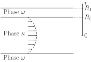
To understand further the physical significance of the dispersion terms appearing in Eq.(25), it is helpful to consider the simple axisymmetric configuration of a tube of radius R1, in which (r,z) represent the radial and axial coordinates
(see Fig.4). The phase (κ) occupies the region 0 < r < R0
Phaseκ Phaseω Phaseω 0 R0 R1 r
FIG. 4. Schematic diagram depicting the cylindrical geometry of the tube problem.
and the phase (ω) occupies R0< r < R1. We impose a
Poiseuille flow in the phase (κ) described by the velocity
v = v0(1 − r
2
R2 0
)ez, and suppose that Dκ = Dω= D is constant
through space. All components of the dispersion tensor, Eq.(25), corresponding to a concentration surface averaged over the width of the tube, vanish except for its axial component Dzz
e which can be written as
Dezz= D − εκh[˜vκ(bκκ+ bκω)]zziκ +εκεω h £ εκεω ¡ Vκκz − Vωωz ¢2+ Vωκz Vκωz ¤. (28) A complete solution to this problem is challenging (see, for example, a discussion of a similar problem in Ref. [65]). Here, our goal is to illustrate the different terms that appear in the dispersion tensor rather than to construct an exact solution. We will therefore use simple approximations and dimensional analysis to develop an approximate solution (a rigorous calculation is performed in the next section for a two-dimensional unit cell). As a first step, we will assume that we can approximate hydrodynamic dispersion using Taylor’s result − D1h[˜vκ(bκκ+ bκω)]zziκ ≈ Pe2 48, (29) with Pe = ¿ v0 µ 1 − r 2 R2 0 ¶Àκ R0 D. (30)
In the limit εω→ 0, this results holds exactly so that we expect
it to be a good approximation for εω sufficiently small. In
addition, we assume that Vκκz ≈ ¿ v0 µ 1 − r 2 R2 0 ¶Àκ ≫ Vκωz ,V z ωω,V z ωκ. (31)
Equation (31) means that we are only considering the physical velocity, and neglect velocity-like terms (such as Vωκ
or Vκω) that appear during upscaling, but do not correspond to
the average pointwise velocity hv0(1 − r
2 R2 0)i κ. Using Eq.(31) yields εκεω h £ εκεω ¡ Vκκz − Vωωz ¢2+ Vωκz Vκωz ¤≈ ε 2 κε2ωD2Pe2 hR20 . (32) The dispersion coefficient can then be written as
Dezz D ≈ 1 + Pe 2µ εκ 48+ ε2κε2ωD hR02 ¶ . (33)
At this point, we need an expression for the exchange coefficient h. This can be determined by computing the closure parameters but is rather tedious. As a simple alternative, we use a dimensional analysis. We know that the exchange coefficient has dimensions (time)−1and corresponds to the inverse of the
time it takes for a molecule of solute to visit the entire domain. We will therefore write h = ADd2,where A is a constant scalar and d is a distance. It yields
Dzz e D ≈ 1 + Pe 2 εκ 48 |{z} Taylor dispersion + ε 2 κε2ω A d2 R2 0 | {z } Two-phase correction . (34)
We remark that (1) we have Dezz
D > 1, for all values of Pe,
because Dκ = Dω= D and h does not depend on v0; (2) the
two-phase correction involves the product εκεωand therefore
disappears in the limit εκ→ 0 or εω→ 0; and (3) with these
approximations, we still obtain dependence on Pe2.
From Eq.(34), we see that the multiphase term acts as a correction to the classical hydrodynamic dispersion. Taylor dispersion arises because of the velocity perturbation within the κ phase, while the multiphase term is a consequence of differences between the mean velocities within each phase. This also suggests that the multiphase dispersion term may contribute to net dispersion in cases for which the velocity contrast is relatively large.
C. Longitudinal dispersion in a simple unit cell
In this section, our goal is to illustrate the behavior of the longitudinal component of the dispersion tensor Dxx
e in a
simple 2D geometry, as described in Fig.5. To compute Dxxe , we could solve numerically the closure problems presented in AppendixB, and use Eq.(25). However, the dispersion tensor may also be written in a more suitable way for computational purposes (see Davit et al. [66] for details):
De Dκ = ε κ[(I + h∇B′κi κ ) − Pehv′κB′κi κ] + εω[DŴ(I + h∇B′ωi ω)], (35)
where L is a characteristic length, B′α= Bα
L, Pe = √ hvκiκ·hvκiκL Dκ , v′ κ = vκ √ hvκiκ·hvκiκ, and DŴ= Dω Dκ. B ′
α solves the following
Periodicity Pressure=1 Periodicity Pressure=0 Periodicity Periodicity Cell cluster ω Channel κ
FIG. 5. Illustrations of the unit cell (εκ ≈ 0.2 and εω≈ 0.8) with
the mesh used for computations inCOMSOL.
10
−210
−110
−110
010
010
110
110
210
210
310
3Pe
D x x e/
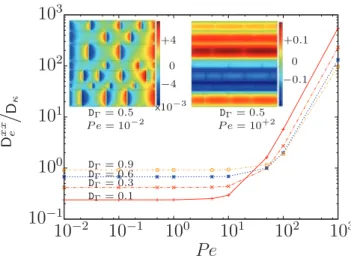
D κ DΓ= 0.9 DΓ= 0.6 DΓ= 0.3 DΓ= 0.1 DΓ= 0.5 P e = 10−2 DΓ= 0.5 P e = 10+2 x10⁻³ 0 +4 −4 0 +0.1 −0.1FIG. 6. (Color online) Logarithmic plots ofDxxe
Dκ as a function of
Pe for different values of DŴ. Solutions of the closure problem for
the x component of B′ωwere calculated numerically usingCOMSOL
MULTIPHYSICS4.2 over the geometry presented in Fig.5. Scalar B′ω,x
fields are presented for DŴ= 0.5, Pe = 10−2(top left) and DŴ= 0.5,
Pe = 10+2 (top right). This figure shows the complex nonlinear
dependence of effective diffusion coefficients upon the system of pa-rameters. For Pe ≪ 1, transport is diffusion dominated. For Pe > 10, hydrodynamic and multiphase dispersion effects become dominant.
boundary-value problem: −εκhv′κi κ = ∇ ·µ DŴ Pe∇B ′ ω ¶ in Vω, (36) ∇· (v′κB′κ) + ˜v′κ+ εωhv′κi κ = ∇ ·µ 1Pe∇B′κ ¶ in Vκ, (37) with the boundary conditions
nωκ· µ 1 Pe∇B ′ κ− DŴ Pe∇B ′ ω ¶ = −nωκ µ 1 Pe− DŴ Pe ¶ on Aωκ (38) and 0 = B′κκ− B′ωκ on Aωκ. (39)
Uniqueness of the solution is obtained by imposing εωhB′ωi ω
+ εκhB′κiκ= 0.
We usedCOMSOL MULTIPHYSICS 4.2 (PARDISO solver) to solve this problem and compute the longitudinal coefficient of the dispersion tensor. The computational mesh is presented in Fig.5, and consisted of triangular meshes (56 570 elements). Solutions were obtained in the following way. First, the velocity and pressure fields were determined by solving the Stokes equations with periodic boundary conditions and a unit pressure difference along the x axis. The resulting velocity field was then used to compute the x component of B′ω (see Fig.6). This field was used in Eq.(35)to determine Dxxe
Dκ for different values of DŴand Pe (see Fig.6). Here, Dexxis rescaled
with Dκ in order to produce results comparable with those of
the experimental literature. However, from a theoretical point of view, Dxx
e should be rescaled with (εκ+ εωDŴ)Dκin order
Our results highlight the complex, nonlinear dependence of the dispersion tensor upon the system of parameters. For Pe ≪ 1, transport is diffusion dominated and only tortuosity affects the longitudinal dispersion coefficient. However, for Pe> 10, hydrodynamic and multiphase dispersion effects become dominant. These results also show that, even for Pe> 1, i.e., in the advection-dominated regime, we have a relatively broad range of P´eclet numbers for whichDexx
Dκ 6 1. In
other words,Dexx
Dκ 6 1 does not necessarily imply that transport
at the microscale is diffusion dominated.
VII. DISCUSSION
Solute transport in biofilms is often described via a notion of effective diffusion, characterized by the ratio De
Daq of effective, De, and reference, Daq≈ Dκ, diffusion coefficients.
As discussed in the Introduction, the definition of this effective diffusion coefficient, as reported in the literature, is ambiguous. In order to provide a clearer definition and to obtain physical insight, we have used the technique of volume averaging to derive three classes of models for solute transport. One of these models, Eq. (24), is an advection-dispersion equation involving an effective dispersion tensor that can be used to interpret the above notion of effective diffusion. In most cases, this one-equation asymptotic model, Eq. (24), is preferable to the other two formulations, i.e., the two-equation and telegrapher’s models. First, it is simple so that it can be easily used to interpret experimental data. Secondly, it has a broad domain of validity, requiring that a time inequality is satisfied, t ≫ εκεω
h , where εα is the volume fraction of
the phase (α = ω,κ) and h is the first-order mass exchange coefficient of the two-equation model (see Sec.V Cfor more details). To appreciate what constraint this inequality poses, consider passive oxygen diffusion in a biofilm of width l = 100 − 1000 µm at temperature 25◦C so that D = 20 ×
10−6cm2 s−1and suppose that there is a purely diffusive flux
at the channel-cluster interface. In this configuration, a good approximation for h−1is the characteristic time for a molecule of solute to diffuse across the entire width of the biofilm, i.e.,
l2
D ≈ 50–500 ms, in which case the previous constraint, for the
validity of the one-equation time-asymptotic model, supplies t ≫ 50–500 ms. Therefore, for a (macroscopic) characteristic time of a few seconds or minutes, the constraint is satisfied.
This model also has a straightforward physical interpreta-tion, and each component of the dispersion tensor, Eq.(25), can be explicitly identified. Two types of dispersion effects are important. One arises from velocity fluctuations within the channels. The other is due to differences in the mean velocities of the two phases. The consequence of these terms, on a macroscopic level, is the facilitation of solute transport within the biofilm, potentially leading to situations for which De/Daq>1. Therefore, our analysis provides a
solid theoretical basis that can be used to interpret data for which De/Daq>1. In addition, Eq. (25) shows that the
effective dispersion tensor depends on the geometry of the channel network. This suggests that parameters describing the geometrical properties of these networks, e.g., their connectivity, may be used in empirical laws for De, in addition
to parameters such as the cell density or the charge of the EPS.
We have also shown that De/Daq<1 does not necessarily
correspond to a diffusion-dominated regime, contrary to what was proposed in Ref. [41]. This is also illustrated in Fig.6, where we observe, in a simple unit cell, that De/Daq<1 for
a broad range of values of the P´eclet number with Pe > 1 (i.e., in the advection-dominated regime).
Interestingly, and to the best of our knowledge, the effect of the macroscopic advective term Ve· ∇hciωκhas not previously
been reported in the literature. One must realize that its effect is extremely difficult to detect, especially in a thin biofilm (typ-ically 100-µm thick). Consider a macroscopic P´eclet number defined by PeM = VeL
De. We remark that, for a characteristic length L which is sufficiently small, the macroscopic advective term may be systematically neglected. Cases for which the advective term may be important correspond to situations in which the channels are oriented parallel to the boundary. In any case, even if this term is negligible, this does not mean
that the effects of advection can be neglected when calculating the net dispersion tensor.
Even though the one-equation advection-dispersion model is straightforward and widely applicable, there are some situations for which a two-equation model or a telegrapher’s model may be more appropriate. Microorganisms within biofilms are known to actively restrict the penetration of antimicrobial agents within the cell clusters [67–69]. For example, positively charged molecules of antibiotics, such as aminoglycosides, can be bound to negatively charged EPS and have limited permeation properties [67]. More recently, Epstein et al. [70] have revealed the extent to which biofilms can limit the penetration of liquids and gas. They measured the contact angle of liquid drops on a Bacillus
subtilisbiofilm and showed that its surface remains nonwetting against up to 80% aqueous solutions of ethanol, surpassing the repellency of Teflon and lotus leaves. Using x-ray computed tomography, they have shown that this biofilm can also be impenetrable to gas. In another study, V´achov´a et al. [71] showed that wild yeast biofilms can develop drug resistance “in which specialized cells jointly execute multiple protection strategies.” In particular, their analysis shows that the cells selectively create permeable EPS, while coordinated efflux pumps actively expel toxic substances outside the cell clusters. These results show that biofilms have the capacity to drastically retard the penetration of antimicrobial agents, and even to actively expel toxic substances. In terms of our modeling approach, this means that the interfacial flux between the channel and cluster phases is modified, for example, by reducing Dω. As a result, the macroscopic mass exchange
coefficient h, between the channels and the cell clusters, can be actively controlled by the microorganisms. If h becomes sufficiently small, the dispersion model discussed previously may cease to be valid for the macroscopic time scale of interest, and the two-equation or telegrapher’s models are needed. Figure7illustrates this temporal behavior. In addition, because we consider abstract phase geometries, these models can be used to describe solute transport in porous media colonized by biofilms. In such systems, biofilms are known substantially to modify mass transport and can be responsible for anomalous behaviours (e.g., in Ref. [72]). Our models can be adapted readily to describe such situations, in the limiting case where the phase (κ) also represents the bulk water phase within the