Chebyshev spectral method for incompressible viscous flow with boundary layer control via suction or blowing

(1)

Chebyshev Spectral Method for Incompressible Viscous Flow

with Boundary Layer Control via Suction or Blowing

by

Giuseppe Alescio

B.Eng., McGill University, Canada (1996) M.Eng., McGill University, Canada (1998)

Submitted to the Department of Aeronautics and Astronautics in partial fulfillment of the requirements for the degree of

Doctor of Philosophy at the

MASSACHUSETTS INSTITUTE OF TECHNOLOGY June 2006

@

A1 Author Departrpent.of Certified by Professor of Certified by IActVrofessk'U Certified by Certified by Accepted by MASSACHUSETTS INSTFTUTE OF TECHNOLOGY

JUL 10 2006

Aeronautics and Astronautics May 26, 2006

Mark Drela Aeronautics and Astronautics Thesis Supervisor

David L. Darmofal Aeronautics and Astronautics

Jaime Peraire I Pvofessoyf Aeronautics and Astronautics

... Ian A. Waitz

rofessor of Aeronautics and Astronautics

Jaime Peraire Professor of Aeronautics and Astronautics Chair, Committee on Graduate Students

(2)

(3)

Chebyshev Spectral Method for Incompressible Viscous Flow

with Boundary Layer Control via Suction or Blowing

by

Giuseppe Alescio

Submitted to the Department of Aeronautics and Astronautics on May 26, 2006, in partial fulfillment of the

requirements for the degree of Doctor of Philosophy

Abstract

The MISES quasi 3-D design/analysis code implements a two-equation integral method with empirical closure relations to solve the boundary layer flow problem with or without suction, but lacks the option of flow control via blowing. The integral method is parameterized with the shape parameter H = */6 which cannot be applied to the blowing problem since 0 -+ 0 downstream of the injection slot causing H - o - a computational disaster.

In this thesis, two alternate approaches are proposed to solve the blowing problem. First, a two-equation integral method parameterized with the profile parameters of a multi-deck representation of a turbulent jet based on Coles' law of the wake was formulated. The appearance of spurious singularities in the Jacobian matrices associated with the system of equations and the vector of unknowns prevented this method from being implemented. Second, a Chebyshev spectral method using the wall function technique was applied to the defect form of the incompressible viscous momentum equation. A turbulent jet profile was computed with N = 40 modes, a number low enough to allow the method's implementation into the MISES framework.

For the spectral approach, a stand-alone code was developed to solve laminar and tur-bulent flow over a flat plate with the following configurations: solid wall, porous wall with vertical suction/blowing, and fluid injection from an inclined slot. For the turbulent case, the Reynolds stress was replaced with a composite model for the eddy viscosity based on Spalding's law of the wall for the inner layer and Clauser's outer layer formulation. In the laminar regime, N - 10 modes are required for an accurate solution whereas the two-layer

structure of a turbulent boundary layer increases this number to N - 100 modes. The

incorporation of a wall function, consistent with the inner layer eddy viscosity model, in the approximation of the streamwise velocity, reduced the required number of modes by an order of magnitude - a major computational advantage.

The more general Spalart-Allmaras turbulence model was implemented in the spectral formulation to investigate the effect of using a wall function based on Spalding's law of the wall. For the flat plate case (solid wall), a small inconsistency between the wall function and the eddy viscosity model produced an erroneous shear stress near the wall. Nevertheless, the velocity profile was in close agreement with an accurate representation constructed from Spalding's law of the wall and Coles' law of the wake.

Thesis Supervisor: Mark Drela

(4)

(5)

Acknowledgments

I am indebted to Professor Drela for suggesting the topic of this thesis, for his guidance and support and, above all, for his patience throughout this endeavour. I would like to thank Professor Darmofal for his critical comments of the work as well as his many suggestions for improvement of the manuscript. Thanks to Professor Peraire for agreeing to serve as both committee member and minor advisor. Thanks to Professor Waitz for continuing to participate in all research meetings despite the shift to a more computationally-oriented project. Special thanks to Professor Sonin for agreeing to be an external reader and for giving me the opportunity to gain valuable teaching experience with his turbulent flow course. Thanks to Dr. Merchant for being an external reader and for always showing an interest in my work. Thanks to Bob Haimes for his expertise with system administration matters. Many thanks to Jean Sofronas for her help in scheduling the defense, for her administration of the lab, and for providing me with a seemingly endless supply of sticky notes. Special thanks to Marie Stuppard for her academic advice. Many thanks to the members of the ACDL (formerly the FDRL) for providing an environment conducive to both learning and having fun. Lastly, I would like to thank my family and friends for their love, support, and encouragement.

(6)

(7)

5.6 Additional Constraints . . . . 5.6.1 Boundary Layer Thickness 5.6.2 Edge Velocity . . . . 5.7 Solver . . . . 5.7.1 Newton Method . . . . . 5.8 Discretization . . . . 5.8.1 Similarity Station . . . . 5.8.2 Logarithmic Differencing . 5.9 Flat Plate . . . . 46 46 47 47 47 48 48 48 48 48 49 49 50 53 53 54 55 58 61 61 61 61 62 62 63 63 63 63 63 63 63 64 64 65 65 65 66 66 66 66 66 66 66 67 67 67 70

(9)

5.9.1 Detailed Plots . . . . 70

5.9.2 Velocity Comparison . . . . 70

5.10 Wall Function . . . . 74

5.10.1 Modified Viscous Streamwise Velocity . . . . 74

5.10.2 Friction Velocity Constraint . . . . 74

5.10.3 Modified Newton System . . . . 75

5.11 Flat Plate Revisited . . . . 76

5.11.1 Detailed Plots . . . . 76

5.11.2 Velocity Comparison . . . . 79

5.12 Flat Plate with Wall Suction or Blowing . . . . 83

5.12.1 Modified Law of the Wall . . . . 83

5.12.2 Modified Inner Layer Eddy Viscosity . . . . 84

5.12.3 Results without Wall Function . . . . 84

5.12.4 Results with Wall Function . . . . 84

5.13 Turbulent Jet . . . . 87

5.13.1 Modified Outer Layer Eddy Viscosity . . . . 87

5.13.2 Modified w. . . . . 87

5.13.3 Results without Wall Function . . . . 87

5.13.4 Results with Wall Function . . . . 87

6 Spalart-Allmaras One-Equation Turbulence Model 91 6.1 Reynolds Stress Transport Equation . . . . 91

6.2 Local Scaling Transformation . . . . 92

6.3 Series Approximation to Working Variable . . . . 92

6.4 Weighted Residual Statement . . . . 92

6.5 Boundary Conditions . . . . 93

6.6 Newton Solver . . . . 93

6.7 Discretization . . . . 95

6.8 Flat Plate . . . . 95

6.9 Wall Function . . . . 96

6.9.1 Modified Viscous Streamwise Velocity . . . . 96

6.9.2 Friction Velocity Constraint . . . . 98

6.9.3 Modified Newton System . . . . 100

6.10 Flat Plate Revisited . . . . 101

7 Conclusion 107 7.1 Summary . . . . 107

7.2 Recommendations for Future Work . . . . 109

A Falkner-Skan Wedge Flows 111 A.1 Boundary Layer Equations in Streamfunction Variables . . . . 111

A.2 Coordinate Transformation . . . . 112

A.3 Variable Transformation . . . . 112

A.4 Requirements for Similarity . . . . 113

A.5 Falkner-Skan Transformation . . . . 113

A.6 Integral Thickness Definitions and Shape Parameter . . . . 114

A.7 Skin Friction Coefficient . . . . 114

(10)

A.9 Spectral Method Results for Wedge Flows . . . . 116

A.9.1 Stagnation Flow (#u = 1) . . . . 117

A.9.2 Constant T (u -= 1/3) . . . . 120

A.9.3 Flat Plate (#u = 0) . . . . 123

A.9.4 Adverse Pressure Gradient (#u = -0.05) . . . . 126

A.9.5 Onset of Separation (3 = -0.088) . . . . 129

B Interacting Boundary Layer Theory for Separated Flows 133 B.1 Integral Boundary Layer Equations . . . . 133

B.1.1 Laminar Flow . . . . 133 B.1.2 Turbulent Flow . . . . 134 B.1.3 Dimensional Form . . . . 134 B.1.4 Dimensionless Form . . . . 135 B.1.5 Logarithmic Form . . . . 136 B.1.6 Similarity Form . . . . 136 B.2 Channel Geometry . . . . 136 B.3 Edge Velocity . . . . 137 B.4 Reynolds Number . . . . 137 B.5 Solution Procedure . . . . 137 B.6 Spectral Formulation . . . . 138

B.7 Laminar Test Cases . . . . 139

B.8 Turbulent Test Cases . . . . 148

(11)

List of Figures

1-1 Aspirated compressor vis-a-vis a blown/aspirated compressor. 1-2 Blowing/suction flow possibilities in a compressor. . . . .

2-1 2-2 2-3 2-4 2-5 2-6 2-7 2-8 3-1 3-2 3-3 3-4 4-1 4-2 4-3 4-4 4-5 4-6 4-7 4-8 4-9 4-10 4-11 5-1 5-2 5-3 5-4 5-5 5-6 5-7 5-8 5-9 5-10 17 18

Multi-deck representation of the jet profile. . . . . 24

Blowing model results: Jet strength Uo/Ujet = 0.085. . . . . 25

Blowing model results: Jet strength un /ujet = 0.59. . . . . 26

Blowing model results: Jet strength uoo/ujet = 0.38. . . . . 27

Layer demarkation lines and entrainment velocities. . . . . 29

Singularities in Jacobian matrices for the jet. . . . . 31

Multi-deck representation of a wake profile. . . . . 32

Singularities in Jacobian matrices for a wake. . . . . 32

Graphs of the Chebyshev polynomials Tk (x), for k = 0,...,5. . . . . 38

Curve-fit results: Jet strength uo/ujet = 0.085. . . . . 40

Curve-fit results: Jet strength un/ujet = 0.59. . . . . 41

Curve-fit results: Jet strength Uo/Ujet = 0.38. . . . . 42

Laminar flat plate: Modal convergence for u/Ue. . . . . 51

Laminar flat plate: Modal convergence for r/r... . . . . 52

Laminar flat plate: Icki vs. k. . . . . 53

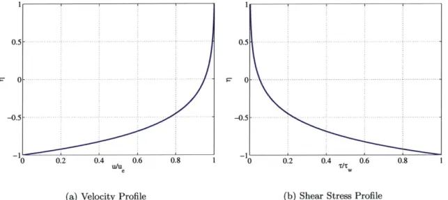
Velocity profiles for a flat plate with wall suction or blowing. . . . . 54

Uniform suction: u/ue and T/T, profiles at ( = 1 m. . . . . 55

Uniform suction: 6, Ue, r, and Cf vs. (. . . . . 56

Uniform suction: P*, 0, H, and Reo vs. . . . . 57

Slot geom etry. . . . 58

Laminar jet: U/Ue and T/Tw profiles at ( = 1 m . . . . 58

Laminar jet: 6, Ue, rw, and Cf vs. (. . . . . 59

Laminar jet: *, 0, H, and Reo vs. . . . . 60

Eddy viscosity blending model. . . . . 65

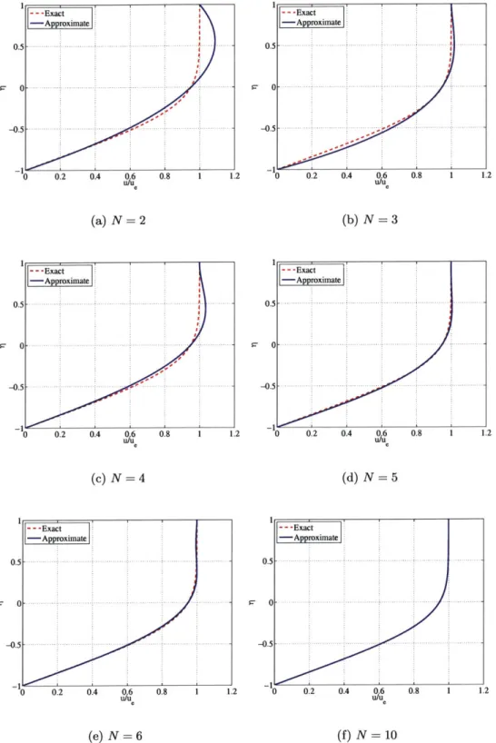
Turbulent flat plate: Modal convergence for u/Ue at = 1 m. . . . . 68

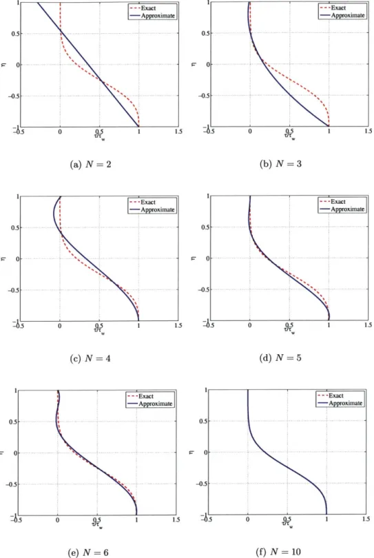
Turbulent flat plate: Modal convergence for r/T at = 1 m. . . . . 69

Turbulent flat plate: 3, Ue, rw, and Cf vs. (. . . . . 71

Turbulent flat plate: P*, 0, H, and Reo vs. . . . . 72

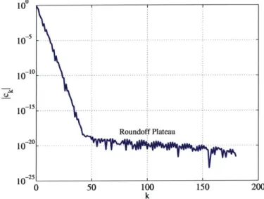
Turbulent flat plate: IckI vs. k at ( = 1 m. . . . . 73

Velocity comparison using inner-law variables u+ and y+.. . . . . . . . 74

Graph of w, vs. (. . . . . 75

Turbulent flat plate (WF): Modal convergence at ( = 1 m. . . . . 76

(12)

5-11 Turbulent flat plate (WF): P*,

0,

H, and Reo vs. (. . . . . 78

5-12 Velocity comparison using inner-law variables u+ and y+ (WF). . . . . 79

5-13 Velocity profile contributions (WF). . . . . 80

5-14 Velocity gradient contributions (WF). . . . . 81

5-15 Shear stress contributions (WF). . . . . 82

5-16 Effect of suction and blowing on logarithmic law of the wall. . . . . 83

5-17 Suction/blowing effect on a flat plate: u+ vs. y+. . . . . 85

5-18 Comparison with Stevenson correlation: u+ vs. y+. . . . . 85

5-19 Suction/blowing effect on a flat plate (WF): u+ vs. y+. . . . . 86

5-20 Comparison with Stevenson correlation (WF): u+ vs. y.. . - . . . . 86

5-21 Turbulent jet: U/Ue and r/T profiles at ( = 1 m. . . . . 88

5-22 Turbulent jet: IckI vs. k at (= 1 m. . . . . 88

5-23 Turbulent jet (WF): u/ue and r/r, profiles at ( = 1 m. . . . . 89

5-24 Turbulent jet (WF): Icki vs. k at (= 1 m. . . . . 89

6-1 Turbulent flat plate: Various profiles at Reo ~ 104. . . . . 96

6-2 Turbulent flat plate: u+ vs. y+ at Re0 ~ 04 . . . . 97

6-3 Turbulent flat plate: Eddy viscosity budget at Reel~ 10 4. . . . . 97

6-4 Turbulent flat plate: IckI vs. k at (= 1 m. . . . . 98

6-5 Graph of vti and vt. . . . . 99

6-6 Graph of wr vs. Avt. . . . . 99

6-7 Turbulent flat plate (WF): Various profiles at Reo ~ 104. . . . . . 102

6-8 Turbulent flat plate (WF): u+ vs. y+ at Reo i 104. . . . 103

6-9 Turbulent flat plate (WF): Eddy viscosity budget at Reo ~~ 104. . . . . 103

6-10 Velocity profile contributions (WF). . . . . 104

6-11 Velocity gradient contributions (WF). . . . . 105

6-12 Shear stress contributions (WF). . . . . 106

A-1 Falkner-Skan velocity profiles for various values of 3.. . . . . 115

A-2 Stagnation flow: U/Ue and r/r, profiles. . . . . 117

A-3 Stagnation flow: 3, ue, Tw, and CJ vs. (. . . . . 118

A-4 Stagnation flow: 3*, 0, H, and Reo vs. (. . . . . 119

A-5 Constant -r: u/ne and /r, profiles. . . . . 120

A-6 Constant r,: 3, Ue, r-, and Cf vs. . . . . 121

A-7 Constant rw: 3*, 0, H, and Reo vs. (. . . . . 122

A-8 Laminar flat plate: u/Ue and r/r profiles. . . . . 123

A-9 Laminar flat plate: 6, Ue, r, and Cf vs. . . . . . 124

A-10 Laminar flat plate: *, 0, H, and Reo vs. (. . . . . 125

A-11 Adverse pressure gradient: u/ne and T/r profiles. . . . . 126

A-12 Adverse pressure gradient: 6, Ue, Tw, and Cf vs. (. . . . . 127

A-13 Adverse pressure gradient: *, 9, H, and Reo vs. . . . . 128

A-14 Onset of separation: u/ue and r/T, profiles. . . . . 129

A-15 Onset of separation: 3, Ue, Tw, and CJ vs. ... . . . . 130

A-16 Onset of separation: 3*, 9, H, and Re0 vs. (. . . . . 131

B-1 Laminar diffuser CBLT, Re = 104: Ue, 0, H, and * - h vs. (. . . . . 140

B-2 Laminar diffuser CBLT, Re = 105: Ue, 9, H, and * - h vs. (. . . . . 141

(13)

B-4 Laminar diffuser CBLT: U/Ue and T/T, profiles at ( = 0.185 m. . . . . 143

B-5 Laminar diffuser IBLT, Re = 104: ue, 0, H, and 6* - h vs. . . . . . 144

B-6 Laminar diffuser IBLT, Re = 105: ue, 0, H, and 6* - h vs. . . . . . 145

B-7 Laminar diffuser IBLT, Re = 106: ue, 0, H, and 6* - h vs. . . . . . 146

B-8 Laminar diffuser IBLT: u/ne and T/r, profiles at ( = 1 m . . . . . 147

B-9 Graph of C, vs. Cp.. . . . . 148

B-10 Turbulent diffuser: ue, 0, H, and * - h vs. (. . . . . 150

B-11 Turbulent diffuser: U/Ue and r/T, profiles at ( = 1 m. . . . . 151

B-12 Turbulent diffuser (WF): ue, 0, H, and 6* - h vs. . . . . . 152

B-13 Turbulent diffuser (WF): U/Ue and T/T, profiles at ( = 1 m . . . . . 153

(14)

(15)

List of Tables

4.1 Falkner-Skan and Spectral Method solutions to flat plate flow . . . . . 53 A.1 Solutions of the Falkner-Skan equation for various values of .. . . . . 115 A.2 Spectral solution to wedge flows for various values of 3.. . . . . 116

(16)

(17)

Chapter 1 Introduction

1.1 Motivation

The viscous/inviscid computational formulation and method of Drela and Giles [10] has become an established tool in the aircraft industry for airfoil design and analysis work. It has since been extended by Youngren [441 with the inclusion of streamtube thickness and rotation effects, permitting application to turbomachinery cascades. Further developments by Merchant [28, 29] have been to include boundary layer suction modeling in both the airfoil and the cascade formulations. Application of these methods to aspirated transonic compressor designs has been extremely successful, as described in Kerrebrock et al. [19, 20]. The ensuing research effort carried out on aspirated compressors in collaboration with the NASA Glenn Research Center has produced more promising designs. For instance, the loading limit with aspiration was doubled in the design of two high pressure ratio fan stages. This result was successfully demonstrated both computationally by Merchant [30] and experimentally by Schuler et al. [37] in MIT's Gas Turbine Laboratory. The aspiration concept has also led to the development of an advanced aerothermal design system which is an essential ingredient in the success of the program.

Figure 1-1: Aspirated compressor vis-a-vis a blown/aspirated compressor.

In an engine environment, however, it may not always be practical to use aspiration without incurring a penalty. The low total pressure in a front fan or first stage of a com-pressor makes it difficult to extract the flow. Alternatively, it may be more feasible to aspirate in high pressure regions of the compressor and blow in low pressure front stages (see Figure 1-1). The performance of a compressor could be improved by utilizing a suit-able combination of both suction and blowing (see Figure 1-2). In order to investigate these alternate designs, flow control via blowing would have to be an added feature in the current suite of computational tools.

(18)

Figure 1-2: Blowing/suction flow possibilities in a compressor.

1.2 Integral Methods for Suction and Blowing

The MISES1 quasi 3-D design/analysis code implements a two-equation integral method with empirical closure relations to solve the boundary layer flow problem with or without suction. The method is parameterized with the shape parameter H = 6*/, where * and 9 are, respectively, the displacement and momentum thicknesses. For flow with or without suction, 3* and 0 are both positive indicating a defect in mass and momentum of the viscous flow relative to the inviscid flow. Conversely, these thicknesses will be negative for a strong blowing case since there is now an excess of mass and momentum in the boundary layer. As the jet dissipates downstream, 6 -> 0 which will cause H -+ 00 - a computational disaster.

The value of the shape parameter is a good indicator of the state of the boundary layer. For a favourable pressure gradient, H is small but for an adverse pressure gradient, H is large. The comparison is usually made relative to the shape parameter values for a flat plate with no pressure gradient and for separated flow. In the laminar regime, H e 2.6 for a flat plate whereas at separation H ~ 4. In the turbulent regime, H J 1.3 for the flat

plate and H ~ 3 at separation. Suction profiles will always have H > 1 and be far from the separation value. For a jet, the shape parameter values are meaningless since the ratio of * to 0 is non-unique.

Solving the blowing problem via the two-equation integral method requires new closure relations. In MISES, the skin friction, Cf, dissipation coefficient, CD, etc. are all functions of the shape parameter H and Reo, the Reynolds number based on 0. These relations are useless for a jet since H -+ 00 as 0 -> 0 and Reo < 0 whenever 0 < 0. Conversely, the suction case requires no changes to these correlations since H > 1 and 0 > 0. In other words, suction is treated in the same fashion as the solid wall case with the exception of performing some record-keeping on the fluid removed from the boundary layer (i.e. source terms in the integral equations).

In Chapter 2, an integral method parameterized with the profile parameters of a multi-deck representation of a turbulent jet based on Coles' law of the wake [6] was proposed. The blowing model does a fairly good job in approximating experimental jet profile data. Consequently, the dimensionless form of both the von Kirmin integral momentum equation and the integral Kinetic Energy (KE) equation were derived for each layer with the closure relations modeled in terms of the profile parameters. It was discovered that the Jacobian matrices associated with the system of equations and the vector of unknowns have spurious singularities. Conversely, applying the model to a wake profile and using the integral ap-proach yields a well-constrained system. Therefore, the application of the integral boundary layer method to compute a multi-deck representation of a turbulent jet profile is inherently

(19)

difficult. An alternate approach would have to be found to efficiently compute the blowing case within the MISES framework.

1.3 Spectral Method with Wall Function

In certain areas of computational fluid dynamics, spectral methods have become the pre-vailing numerical tool for large-scale computations [17]. The three-dimensional direct sim-ulation of homogeneous turbulence, computation of transition in shear flows, and global weather modeling are typical examples. For many other applications, such as heat transfer, boundary layers, reacting flows, compressible flows, and magnetohydrodynamics, spectral methods have proven to be a viable alternative to the finite-difference and finite-element techniques.

Spectral methods are characterized by the expansion of the solution in terms of global and usually, orthogonal polynomials. Although originating in early-20th-century work of Galerkin and Lanczos, numerical spectral methods for partial differential equations (PDEs) were first developed by meteorologists in the 1950s. The expense of computing nonlinear terms remained a severe drawback until the early 1970s when Orszag [31] and Eliasen et al. [12] developed the transform methods that still form the backbone of many large-scale spectral computations.

These methods and others used in fluid mechanics prior to 1970 are termed spectral Galerkin methods. The fundamental unknowns are the expansion coefficients and the equa-tions for these are derived by the techniques used in classical analysis. With the advent of the computer, an alternate discretization was made possible. Termed the spectral colloca-tion technique, the fundamental unknowns are the solucolloca-tion values at selected collocacolloca-tion points and the series expansion is used solely for the purpose of approximating derivatives. This approach was proposed by Kreiss and Oliger [22] and by Orszag [32] in the early 1970s. Boyd [2]) divides spectral methods into two broad categories using a more generic clas-sification: interpolating and non-interpolating. The interpolating methods (comprised of the collocation or pseudospectral methods) associate a grid of points with each basis set. The coefficients of a known function are found by requiring that its truncated series agree with it at each point in the grid. In the case of a PDE, the associated residual is forced to vanish at each collocation point. The non-interpolating category includes Galerkin's method and the Lanczos tau-method [23]. There is no grid of interpolation points. Instead, the coefficients of a known function are computed by multiplying its truncated series by a given basis function and integrating. For a PDE, the residual is weighted by a given basis function and integrated.

In Chapter 3, the use of a Chebyshev spectral formulation (Galerkin-type approach) to curve-fit experimental turbulent jet profiles obtained from Zhou and Wygnanski [45] demonstrated that few modes are required to capture the outer layer profile. The inner layer could then be approximated using an appropriate wall function to complete the profile. The wall function technique is a common strategy employed in current Navier-Stokes methods to reduce the grid density requirements in the near-wall region. Spalding's law of the wall [39] is a good candidate since it captures the turbulent inner layer profile for flat plate flow and it has an eddy viscosity model associated with it.

The Galerkin form of the Chebyshev spectral method formulated with the defect form of the incompressible viscous momentum equation was developed. Application of the method to laminar flow over a flat plate with or without flow control was successful, as shown in

(20)

Chapter 4. The solution to the analogous turbulent flow problem, described in Chapter 5, required a large number of Chebyshev modes due to the two-layer structure of the boundary layer. An algebraic model for the eddy viscosity based on Spalding's law of the wall for the inner layer and Clauser's outer layer formulation [5] was implemented. Including a wall function in the velocity approximation that is consistent with the inner layer eddy viscosity model drastically reduced the number of Chebyshev modes. In the jet case, the number of modes is low enough to have the method coded into the MISES framework thus allowing design and analysis work on cascades with flow control via blowing.

1.4 Thesis Objective

The main objective of this thesis is:

9 To develop a computationally efficient model for boundary layers with blowing in order to extend the capability of the MISES code to design turbomachinery cascades with this flow control method.

1.5 Contributions

The following is a summary of the main contributions of this thesis:

" First demonstration of the inherent difficulties of applying the two-equation integral method to solve the blowing problem with a multi-deck representation of a turbulent jet velocity profile based on Coles' law of the wake.

" First application of the Galerkin form of the Chebyshev spectral method to the defect form of the incompressible viscous momentum equation. Results for laminar and turbulent flow over a flat plate with or without boundary layer control are in excellent agreement with theory and/or experiment.

" First incorporation of Spalding's inner layer eddy viscosity model, in conjunction with Clauser's outer layer formulation, within an algebraic turbulence model for the spectral method described previously.

" First application of the wall function technique for the spectral method described previously. An order of magnitude reduction in Chebyshev modes is observed for all the test cases. Such a drastic drop in the number of modes can only be achieved if the wall function is consistent with the inner layer eddy viscosity model.

" First incorporation of the Spalart-Allmaras turbulence model within the spectral for-mulation as applied to the flat plate case with no flow control. The inconsistency be-tween the wall function based on Spalding's law of the wall and the Spalart-Allmaras eddy viscosity is observed with an erroneous shear stress near the wall.

1.6 Overview

The thesis is structured in the following manner. Chapter 2 applies the integral method to a blowing model and spurious singularities are discovered in the Jacobian matrices associated

(21)

with the system of equations and the vector of unknowns. Chapter 3 presents the Galerkin form of the Chebyshev spectral method and applies it to a curve-fitting example. Chapter 4 applies the spectral method to solve the laminar incompressible boundary layer flow problem over a flat plate with or without flow control. Chapter 5 solves the analogous turbulent flow problem using an algebraic model for the eddy viscosity and then demonstrates the reduction in modes achieved with the incorporation of a wall function in the velocity approximation. Chapter 6 describes the Spalart-Allmaras turbulence model and applies it to the flat plate case with no flow control. Chapter 7 summarizes the contributions of the thesis and offers a few recommendations for future work. Appendix A presents the Falkner-Skan wedge flows which are used for comparison purposes with the spectral solution. In Appendix B, boundary layer separation in a diffuser is computed via the two-equation integral method and the results are compared to those obtained from the spectral formulation.

(22)

(23)

Chapter 2 Integral Method

An integral method parameterized with the profile parameters of a multi-deck representa-tion of a turbulent jet based on Coles' law of the wake [6] is proposed. The blowing model does a fairly good job in approximating experimental jet profile data. Consequently, the dimensionless form of both the von Kairmin integral momentum equation and the integral Kinetic Energy (KE) equation are derived for each layer with the closure relations modeled in terms of the profile parameters. It was discovered that the Jacobian matrices associ-ated with the system of equations and the vector of unknowns have spurious singularities. Conversely, applying the model to a wake profile and using the integral approach yields a well-constrained system. Therefore, the application of the integral boundary layer method to compute a multi-deck representation of a turbulent jet profile is inherently difficult.

2.1 Blowing Model

Consider modeling a turbulent jet profile using a multi-deck representation as shown in Figure 2-1. Coles' law of the wake [6] is used to express the velocity profile in each layer given by

Top u=uy+(Ue-Uy) 1 - cos

(rg-y

, Y y 6,

(2.1)

Bottom u = uo

+

(Uy - Uo)) [1 - cos

(7r)]

0 < y ! Y.

In these expressions, uo and uy are, respectively, the streamwise velocities at y = 0 and y = Y. The boundary layer thickness is denoted by 6 and ue is the edge velocity (streamwise component).

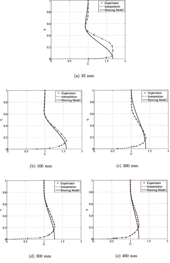
This simple model was applied to sets of turbulent jet profiles obtained from experiments conducted by Zhou and Wygnanski [45] as shown in Figures 2-2 to 2-4. The data from three jet strengths uOo/ujet _{= {0.085,0.59,0.381 each consisting of five profiles measured at 32,}

100, 200, 300, and 400 mm from the slot location were used.

The experimental jet velocity was first normalized with its edge velocity such that Uexp

uexp/ue. Next, the MATLAB1 piecewise cubic Hermite interpolation technique was used to approximate the profile with 181 points. The points were chosen by setting x = - cos O with p ranging from [0, 7r] in increments of 7r/180 and then applying the transformation

y = (x + 1) /2 such that 77 = y/6 ranges from [0, 1]. Using the interpolated jet velocity 'The Mathworks, Inc., Natick, MA, http://www.mathworks.com

(24)

y y Ue Y Y U Uy IPU _U 0 0 U

Figure 2-1: Multi-deck representation of the jet profile.

Uint = Uint/Ue, the maximum velocity in each profile was set to U0 = uo/ue whereas the

minimum velocity in the outer layer was set to Uy = uy/ue. The location of Uy will be

Y/6 in the normalized q coordinate. Hence, the model profiles can be constructed and

compared.

Overall, the blowing model does a fairly good job of approximating the experimental profiles. Figure 2-2 is a pathological case for the model since Y = 6 (where uy = ue). The top layer cannot be used since the denominator of the cosine function blows up. The same would be true for the bottom layer if Y = 0 (where uy = uo). Figures 2-3 and 2-4 represent the types of profiles the model was intended to predict. Due to this close agreement between model and experiment, there was substantial motivation to attempt to include blowing in an integral formulation.

2.2 Integral Boundary Layer Equations

2.2.1 Turbulent Flow

The 2-D, steady, incompressible Reynolds-averaged continuity and x-momentum thin shear layer equations governing the real viscous flow (RVF) in the turbulent regime are given by

u+

= 0 _(2.2)

ax ay

a

2

1 I p

1 ar

(92)

+ a(UV) +

=9

0.(2.3)

In these expressions, u and v are, respectively, the x- and y-components of the RVF velocity;

p is the mass density; p is the static pressure and T is the shear stress given by

T = p -

pu'v,

(2.4)

ay

where p is the dynamic viscosity and -pu'v' is the turbulent shear (or Reynolds stress).

2.2.2 Dimensional Form

(25)

(a) 32 mm

1

Experiment * Experim

- -Interpolation - - Interpol -Blowing Model 0.8 -Blowin

0.6-0.4 .. .. -.. -.-.-- .- -.. -- ---.- -..- 0 .4 - -.--.--- - 0.2-5 10 15 0 5 10 U U (b) 100 mm (c) 200 mm * Experiment * Experime - - -Interpolation - - -Interpola

-Blowing Model -Blowin

- -. -. --. -- 0 .6 - - - - - -.-- -. -. -- - - 0 .4 -. - -.-..-- . - -... -. 0 .2 - - - -5 10 15 0 5 10 U U (d) 300 mm (e) 400 mm

Figure 2-2: Blowing model results: Jet strength uoo/ujet = 0.085.

(26)

(a) 32 mm 11 Experiment * Experi - --Interpolation - - -Interx 0.8 -Blowing Model 0.8---0.6 -- --- - - - - 0.6 -0 .4 - - - --.-.-.- - .- - 0 .4 - -.-.-.- . - -.-0.2 - 0.2 ---- - -0 0.5 1 1.5 2 0 0.5 1 1.5 U U (b) 100 mm (c) 200 mm 1 1 * Experiment * Experti - - -Interpolation - - -Interpo

0.8-- -- Blowing Model 0.8 -Blowin

0 .6 -- - -- -- - - -- - - -- 0 .6 --0.4 - -0.4-.2- --- -- ---- -.--- - --* * 0 0.5 1 1.5 2 0 0.5 1 1.5 U U (d) 300 mm (e) 400 mm

(27)

(a) 32 mm

e Experiment * Experiment

-- Interpolation --- Interpolation

-Blowing Model 0.8 -Blowing Model

- 0.6 - - -.-.-0.4 ---... -. -. -. -- 0 .2 - - - -0.5 1 1.5 2 2.5 3 0 0.5 1 1.5 2 2.5 3 U U (b) 100 mm (c) 200 mm e Experiment * Experiment - -Interpolation - -Interpolation

-Blowing Model 0.8 -Blowing Model

0.6 -. -. -. -. _{0 .4} --- -- . -- - 0 .2 0.5 1 1.5 2 2.5 3 0 0.5 1 1.5 2 2.5 3 U U (d) 300 mm (e) 400 mm

(28)

j [U (Y2 - Ue) X (2.2) + (2.3)] dy, (2.5)

/1

jY2 [(2 - u2) x (2.2)

+

2u x

(2.3)]

dy, (2.6)

yields the dimensional form of both the von Kirman integral momentum equation and the integral Kinetic Energy (KE) equation

±

(pe) + peUe6d -i + T2 = p2E2 (Ue - U2) - p1E1 (Ue -ui), (2.7)

dd

d (pene0*) 2D - 2u1T1 + 2u2T2 = p2E2 (u2 - u) - p₁E₁ (u2 - u). (2.8)

These equations involve the standard integral definitions for the displacement thickness *, momentum thickness 0, and KE thickness 0* given by

* 1 - u ) dy, (2.9)

SY2(U Udy, (2.10)

JYi Ue Ue

6* (1 -2) dy. (2.11)

Y1 Ue Ue

The shear dissipation D and entrainment velocity E, which is the velocity component normal to the demarkation line Y (x) as shown in Figure 2-5, are defined by

lu

oudY

D T-audy and E = u - v. (2.12)

y1 ay dx

The pressure gradient term has been written in terms of the edge velocity ue. This comes from the assumption that in a boundary layer

P (X, Y) p() = Pe (), (2.13)

where Pe (x) is the static pressure at the edge and using Bernoulli, it can be shown that

dPe _due

(2.14)

dx d

The edge density pe = p since the flow is incompressible.

For a single (solid) wall boundary layer, the integration is typically performed across the entire layer. In this case, Yi is at the wall where ui = Ei = 0 and Y2 is outside the

layer where Ue - U2 = T2 = 0. This results in both righthand sides being zero and gives the more familiar entrainment-free forms of these equations. For multi-deck representations of confluent shear layers the entrainment terms will be present. Moreover, if flow control via blowing occurs over a slot (usually inclined at some angle and flush with the surface), the no-slip condition will not hold. Over the slot, ui = um and vi = v, which are, respectively, the

(29)

y 4 Y₂(X) -y Y- ------ ~ -... - - - -- ---El V2 U 2

Figure 2-5: Layer demarkation lines and entrainment velocities.

The governing equations for the blowing model can be derived by performing two in-tegrations. First, integrate from Yi = 0 to Y2 = Y to obtain the governing equations for

the bottom layer. Second, integrate over the entire layer and remove the respective von Karmain integral momentum and KE integral equations from the bottom layer to obtain the top layer equations. Lastly, express these equations in dimensionless form as required in the MISES framework.

2.2.3 Dimensionless Form

The dimensionless form of both the von Kirmain integral momentum equation and the integral KE equation governing the entire boundary layer for the blowing case are

dO

_-2+

6*

_{--- +2)}

9

due PwVw

_{1 -}

u +Cf

+

dx / ue dx peue e 2

dO*

9*

due _ PwVw

dx ue dx PeUe

whereas the bottom layer is governed by

dOy (6y +2Cy due pyEy

+ +L2

dx Oy ue dx Peue

dOy d +3' 0y due - pyEy uy ₊

dx Ue dx Peue Uel uw uw u- + Cf + 2CD ue )Ue U- + Pe1e U ue pene Ue )

Cf

2 pwom ₁ u uW - + -Cf + 2CDy. PeUe Ue) Ue (2.15) (2.16) (2.17) (2.18) The skin friction Cf and dissipation coefficient CD are defined by

E2

(30)

Tw CJa 1 TP2 2Peue D and CD =D 3' Peue (2.19)

where T is the shear stress at the wall given by

(2.20)

Tw =-p

y -o

The Y subscript on the terms 5y, Oy, 0y and CDy indicates that the limits of the integration go from 0 to Y. The entrainment velocity at the height Y is denoted Ey. The term pwVw represents the injected mass flux and u, is the streamwise velocity component of the injected

fluid.

2.3 Inherent Difficulties

For the blowing case, the vectors of unknowns and profile and W given by

0- y

1

U= _*

6y . Yv .

parameters are, respectively, U

Y

and W = .

Uy .UO _ Appropriate closure relations can be modeled for Cf, CD,

that the governing equations can be expressed as

Ey, etc. (2.21) in terms of W such

d

V (W) =f (W),

dx (2.22)

where the vector V is given by

0- Oy

0

* -0* V =

.

L _ By performing the chain rule and inverting yields

dW

V

-(

dx

= [(W)V,

fawJ

(2.23)

(2.24) where [8V/8W] is the Jacobian matrix for the system of equations. Furthermore, since U = g (W) then to determine W given U requires [U/W]- 1_{. The term [OU/&W] is the}

Jacobian matrix for the vector of unknowns.

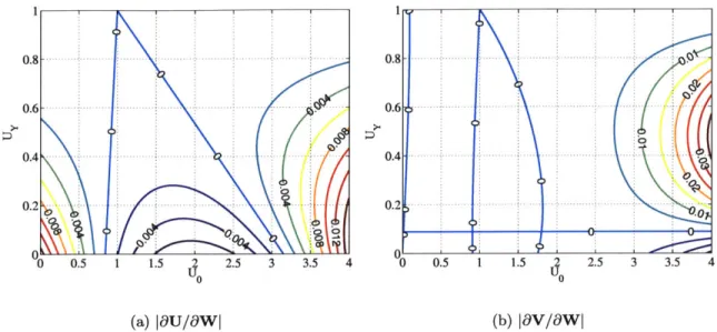
It turns out that both these Jacobian matrices have spurious singularities as shown in Figure 2-6. These contour plots were obtained by varying Uo in the range [0, 4] and Uy in the range [0, 1]. The ratio Y/6 = 0.2 with 6 being set to unity. The value of 6 is required since the integral thicknesses are lengths.

(31)

2 2.5 3 3.5 4 U0 (a) |U/|Wl 0.5 1 1.5 2 2.5 3 3.5 4 U0 (b) |BV/Wl Figure 2-6: Singularities in Jacobian matrices for the jet.

2.4 Wake Model Comparison

As a means of comparison, the idea to model the jet profile with a two-layer velocity deck was applied to a wake profile as shown in Figure 2-7. In this case, the expression for the velocity profile in each layer is given by

u = uO+ + (ue - uo+) 1 [1 - cos (7r F)]

U = UO- + (Ue - uo-) 1 [1 - cos (7r

o

<

Y:5

6+,

6

_{- <y :5 0.}

In these expressions, uO+ and uo- are, respectively, the streamwise velocities at y = 0 for the top and bottom layers. The boundary layer thicknesses are denoted 6+ and 6. Note that these thicknesses cannot be zero or else the cosine function in the velocity expression for their respective layers will blow up. Furthermore, if uO+ = Ue or uo- = Ue, both 6+ and

6- will be ill-defined.

For the wake case, the vectors of unknowns and profile parameters are, respectively, U and W given by

6

- O' Oo . 00 .

and

W=[

.

UO+

_UO-In these expressions the 0 subscript indicates that the limits of the integration go from to 0. Thicknesses with no subscript have been integrated over the entire layer or from 6-to 6+. Furthermore, UO+ = UO+

/Ue

and UO- = uo- /ue.

Following the same arguments as the blowing case, the vector V is given by Top

Bottom

(2.25)

(32)

Y lie 0 u0+ . U 0 00 UO U -Y I U e

Figure 2-7: Multi-deck representation of a wake profile.

0* - 0*

V = 0 0 (2.27)

60

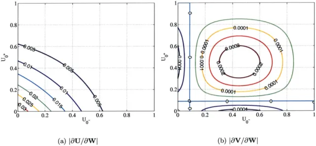
and the contour plots of the Jacobian matrices are shown in Figure 2-8. In this case, both UO- and U0+ were varied in the range [0, 1]. The height 6+ was set to unity and 6~ = -J+. The Jacobian matrix [OU/OW] has no spurious singularities whereas [aV/8W] has singularities at UO- = Uo+ = (-5 + 2V/iU) /15.

0.8|-0.6 0.4 0.2 00 0.2 0.4 U- 0.6 0.8 1 0-0 0-0.2 0.4 UO_0 . 08 1 (a) |iU/OW| 0D U-₀ (b) |BV/OWI Figure 2-8: Singularities in Jacobian matrices for a wake.

X?> e 00

(33)

2.5 Perturbation Analysis

In order to gain some insight as to what the singularities in [OV/OW] mean to the set of integral equations, consider a perturbation 6V due to the perturbation 3Wv such that

6V

=a

Ae6WV, (2.28)

14W

where A and e are, respectively, the diagonal matrix of eigenvalues and the matrix of eigenvectors associated with [8V/aW]. Denoting the zero eigenvalue corresponding to each singularity as Ao and its associated eigenvector as eo, the perturbation 6U will be

6U = eo WV . (2.29)

aww

For the wake, both singularities in [8V/8W] produce a nonzero perturbation in the displacement thicknesses for each layer. Recall that in reality the edge velocity ue, assumed given here, does depend on the displacement thickness P*. In fact, computing the flow past separation is only possible with Interacting Boundary Layer Theory (IBLT) where the governing equation for ue is written in terms of P* and the geometry of the problem (see Appendix B). In Classical Boundary Layer Theory (CBLT), ue is prescribed and the computation fails at the separation point due to the Goldstein singularity. Therefore, although [V/&W] has spurious singularities, the governing equation for ue will prevent the Jacobian matrix for the entire system of equations from being singular for the wake case.

In the blowing case, both [8U/&W] and [aV/8W] have spurious singularities. Apply-ing the above analysis to [aV/8W] yields zero perturbations in both the momentum and displacement thicknesses for each layer. Hence, the Jacobian matrix for the entire system of equations will be singular. Therefore, using a two-equation integral boundary layer method to compute the multi-deck representation of a turbulent jet profile is inherently difficult. In the following chapters, an alternate approach is taken to efficiently compute the blowing case within the MISES framework.

(34)

(35)

Chapter 3 Spectral Method

In this chapter, the Galerkin form of the Chebyshev spectral method is presented. By using the idea of a residual, it will be shown how spectral approximation can be defined for the representation of a given function as well as for the solution of a partial differential equation (PDE). The boundary conditions will be imposed by means of the tau method. The Chebyshev polynomials will be defined and their orthogonality property examined. Lastly, the methodology will be applied to solve a simple curve-fitting example. The notation used in the formulation has been adopted from Peyret [33] and Boyd [2].

3.1 Basic Idea

Spectral methods are encompassed within the framework of the method of weighted resid-uals (MWR) as described in Finlayson [14]. This family of methods for solving PDEs utilize approximations defined in terms of a truncated series expansion, such that some quantity (error or residual) which should be identically zero is forced to be zero only in an approximate (mean) sense. This is done through the inner product defined by

lb

where u (x) and v (x) are arbitrary functions defined on [a, b] and w (x) is some given weight function.

3.2 Function Approximation

Assume the function u (x) defined on [a, b] can be approximated by a truncated series expansion

N

u (x) uN (X) ~~ Ck k (X) ,

(3.2)

k=O

where the N + 1 basis (or trial) functions

#k

(x) are given and the series coefficients ck must

be determined. In spectral methods, the chosen basis functions are either trigonometric functions eikx (i.e. Fourier series) for spatially periodic problems or Chebyshev Tk (x) and Legendre Pk (x) polynomials for nonperiodic problems. In general, the trial functions are orthogonal with respect to some weight w (x), such that

(36)

where Ck = constant and 4k1 is the Kronecker delta symbol.

The aforementioned basis functions possess two other useful properties. First, they are easy to compute. Indeed, both trigonometric functions and polynomials fulfill this criterion. Second, they form a complete set. To satisfy this property, the basis functions must be sufficient to represent all functions in the class we are interested in with arbitrarily high accuracy.

When the series UN (x) is substituted into the PDE

Lu (x) =

f

(x), (3.4)

where L is either the linear or nonlinear homogeneous differential operator associated with the PDE under consideration and

f

(x) is the corresponding inhomogeneous term, the result

is the residual function defined by

RN (x) LUN (x) -

f

(x) (3.5)

The residual function RN (x) is identically equal to zero for the exact solution. The difficulty lies in choosing the series coefficients cl in such a way so as to minimize the residual function.

3.3 Method of Weighted Residuals

The MWR sets to zero the inner product

(RN, Nj) =

Ja

RN (X) Oj (x) w* (x) dx = 0, (3.6) where /j (x) are the test (or weighting) functions and the weight w, (x) is associated with

the method and basis functions. Note that

j

E JN where the dimension of the discrete set

JN depends on the problem under consideration.

The choice of the test functions and of the weight defines the method. The Galerkin-type approach corresponds to the case where the test functions are the basis functions themselves and the weight w., is the weight associated with the orthogonality of the basis functions, that is,

0j = #$ and w* = w. (3.7)

3.4 Boundary Conditions

The traditional Galerkin method applies when the basis functions k (x) in the expansion of UN (x) satisfy the homogeneous boundary conditions of either Dirichlet, Neumann, or Robin type. In this case, JN =

{0,...

, N} which furnishes N + 1 Galerkin equations of

the form (3.6) to determine the N + 1 series coefficients ck. If the basis functions do not satisfy the homogeneous boundary conditions, the method may be applied by first using basis recombination. However, it is usually simpler to use the tau method.

In 1938, Lanczos [23] introduced the tau method to allow the use of basis functions not satisfying the homogeneous boundary conditions. Basically, this technique replaces Galerkin

36

(37)

equations with boundary conditions. For instance, if there are two boundary conditions then

JN =

{o,

...

, N - 2}. The omission of the Galerkin equations for

j

= N - 1 and

j

= N

introduces a supplementary error, the tau error, which has given its name to the method. The reader is referred to Gottlieb and Orszag [15] and Canuto et al. [3] for further details. In brief, high order derivatives of Chebyshev (and Legendre) polynomials grow rapidly as the endpoints are approached. The mismatch between the large values of the derivatives near x i 1 and the small values near the origin can lead to poorly conditioned matrices and accumulation of roundoff error. However, the ill-conditioning of an uncombined basis is usually not a problem unless N - 100 or the PDE has third or higher derivatives.

3.5 Chebyshev Polynomials

The Chebyshev polynomial of the first kind Tk (x) is the polynomial of degree k defined for x E [-1, 1] by

Tk (x) = cos (k cos 1 x) , (3.8)

where k = 0, 1, 2..., and hence -1 < Tk (x) 1. Now, setting x = cos z yields

Tk (z) cos kz, (3.9)

from which it is a simple matter to obtain the first Chebyshev polynomials

To (x) = 1, Ti (x) = cos z = x, T2 (x) = cos 2z = 2cos2 z - 1 = 2x2 - 1 ... (3.10)

Alternatively, using the trigonometric identity

cos (k

+

1) z

+

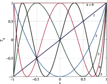
cos (k - 1) z = 2 cos z cos kz (3.11) the following recurrence relation can be deduced

Tk+1 (x) = 2xTk (x) - Tk_1 (x), (3.12) where k > 1. The polynomials Tk (x) for k > 2 can be obtained from the knowledge of To (x) and T1 (x). The graph of the first few polynomials is shown in Figure 3-1.

Consequently, the recurrence relations for the first, second, and higher order derivatives of the Chebyshev polynomials can be determined by simple differentiation. For instance, the first and second derivative recurrence relations are given by

Tk+1 (x) = 2Tk (x) + 2xTk (x) - T_ 1 (x), (3.13)

Tj'+1 (x) = 4Tk' (x) + 2xTk' (x) - Tk'_1 (x) . (3.14)

The Chebyshev polynomials are orthogonal on [-1, 1] with the weight

1

-( = . (3.15)

(38)

05.51

1 -0.5 0 05 5

X

Figure 3-1: Graphs of the Chebyshev polynomials Tk (x), for k =0, . . ., 5.

(Tk, Ti), Tk (x) T (x) w (x) dx = Ck (3.16)

where Ck takes on the values

Ck = (3.17)

3.6 Curve-Fit Example

Consider curve-fitting sets of turbulent jet profiles obtained from experiments conducted by Zhou and Wygnanski [45] using the spectral method. Once again, the data from three jet strengths Uoo/Ujet = {0.085,0.59,0.38} each consisting of five profiles measured at 32, 100, 200, 300, and 400 mm from the slot location were used.

The experimental jet velocity was first normalized with its edge velocity such that Uexp = Uexp/Ue. Next, the MATLAB piecewise cubic Hermite interpolation technique was used to

approximate the profile with 181 points. The points were chosen by setting x = - cos W with W ranging from [0, 7r] in increments of 7r/180 and then applying the transformation 77 = (x + 1) /2 such that 77 = y/6 _{ranges from [0, 1]. The interpolated}_jet_{velocity Uint}₌_Uint/ue

is denoted U (77) defined on [0,11 and its truncated series expansion UN (7q) has the form

N

UN () k k (C).- (3-18)

k=O

Choosing the basis functions

#k

(77) to be the Chebyshev polynomials Tk (x) defined on

[-1, 1] requires a change of variable from 77 to x given by

Chebyshev spectral method for incompressible viscous flow with boundary layer control via suction or blowing

Chebyshev Spectral Method for Incompressible Viscous Flow

with Boundary Layer Control via Suction or Blowing

Giuseppe Alescio

@

JUL 10 2006

rofessor of Aeronautics and Astronautics

Chebyshev Spectral Method for Incompressible Viscous Flow

with Boundary Layer Control via Suction or Blowing

Abstract

Acknowledgments

Contents

List of Figures

0,

List of Tables

Chapter 1

Introduction

1.1

Motivation

1.2

Integral Methods for Suction and Blowing

1.3

Spectral Method with Wall Function

1.4

Thesis Objective

1.5

Contributions

1.6

Overview

Chapter 2

Integral Method

2.1

Blowing Model

(rg-y

+

(7r)]

2.2

Integral Boundary Layer Equations

u+

a

2

1

I p

1 ar

(92)

+ a(UV) +

=9

pu'v,

ay

/1

+

(2.3)]

±

oudY

-2+

--- +2)

9

1 -

+

dO*

9*

Cf

2.3

Inherent Difficulties

1

d

V (W) =f (W),

0

dW

V

-(

dx

= [(W)V,

fawJ

2.4

Wake Model Comparison

o

<

Y:5

6+,

_-2+

_{--- +2)}

_{1 -}

_{- <y :5 0.}