Alfvénic fluctuations in "newborn"' polar solar wind

HAL Id: hal-00317803

https://hal.archives-ouvertes.fr/hal-00317803

Submitted on 3 Jun 2005

HAL is a multi-disciplinary open access

archive for the deposit and dissemination of

sci-entific research documents, whether they are

pub-lished or not. The documents may come from

teaching and research institutions in France or

abroad, or from public or private research centers.

L’archive ouverte pluridisciplinaire HAL, est

destinée au dépôt et à la diffusion de documents

scientifiques de niveau recherche, publiés ou non,

émanant des établissements d’enseignement et de

recherche français ou étrangers, des laboratoires

publics ou privés.

Alfvénic fluctuations in ”newborn”’ polar solar wind

B. Bavassano, E. Pietropaolo, R. Bruno

To cite this version:

B. Bavassano, E. Pietropaolo, R. Bruno. Alfvénic fluctuations in ”newborn”’ polar solar wind. Annales

Geophysicae, European Geosciences Union, 2005, 23 (4), pp.1513-1520. �hal-00317803�

Geophysicae

Alfv´enic fluctuations in “newborn” polar solar wind

B. Bavassano1, E. Pietropaolo2, and R. Bruno1

1_{Istituto di Fisica dello Spazio Interplanetario, Istituto Nazionale di Astrofisica, Rome, Italy} 2_{Dipartimento di Fisica, Universit`a di L’Aquila, L’Aquila, Italy}

Received: 27 January 2005 – Revised: 30 March 2005 – Accepted: 5 April 2005 – Published: 3 June 2005

Abstract. The 3-D structure of the solar wind is strongly

de-pendent upon the Sun’s activity cycle. At low solar activity a bimodal structure is dominant, with a fast and uniform flow at the high latitudes, and slow and variable flows at low lat-itudes. Around solar maximum, in sharp contrast, variable flows are observed at all latitudes. This last kind of pattern, however, is a relatively short-lived feature, and quite soon after solar maximum the polar wind tends to regain its role. The plasma parameter distributions for these newborn polar flows appear very similar to those typically observed in po-lar wind at low sopo-lar activity. The point addressed here is about polar wind fluctuations. As is well known, the low-solar-activity polar wind is characterized by a strong flow of Alfv´enic fluctuations. Does this hold for the new polar flows too? An answer to this question is given here through a comparative statistical analysis on parameters such as total energy, cross helicity, and residual energy, that are of general use to describe the Alfv´enic character of fluctuations. Our results indicate that the main features of the Alfv´enic fluc-tuations observed in low-solar-activity polar wind have been quickly recovered in the new polar flows developed shortly after solar maximum.

Keywords. Interplanetary physics (MHD waves and

turbu-lence; Sources of the solar wind) – Space plasma physics (Turbulence)

1 Introduction

The 3-D structure of the solar wind dramatically changes during the Sun’s activity cycle. This feature, first seen in wind speed values estimated from interplanetary scintillation observations (e.g. Rickett and Coles, 1983), has been unam-biguously confirmed by in-situ measurements of Ulysses, the first spacecraft able to perform an almost complete latitudinal scan (about ±80◦) of the heliosphere. From the beginning

Correspondence to: B. Bavassano

(bavassano@ifsi.rm.cnr.it)

of its journey away from the ecliptic plane in February 1992, through a Jupiter gravity assist, Ulysses has performed obser-vations for more than an entire solar activity cycle, with two full out-of-ecliptic orbits completed in mid-2004. From this huge data set it comes out very clearly that at low solar activ-ity the solar wind has quite a simple bimodal structure, with a fast, tenuous, and uniform flow filling large angular sectors at high heliographic latitudes (the so-called polar wind) and slower, more variable, and highly structured flows at low lati-tudes (e.g. McComas et al., 1998, 2000). Around solar maxi-mum, in sharp contrast, variable flows are observed at all lati-tudes and the wind structure appears to be a complicated mix-ture of flows coming from a variety of sources (McComas et al., 2002, 2003). However, this kind of wind pattern per-sists for a relatively short fraction of the high-solar-activity phase. For the remainder of the cycle a bimodal structure is the dominant feature of the 3-D solar wind.

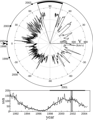
All this is well illustrated by Figs. 1 and 2, referring to the first and the second out-of-ecliptic orbit of Ulysses, re-spectively. The latitudinal variation of the wind velocity is displayed in the top polar graphs, with time running anti-clockwise from the left arrow. Note that the angular resolu-tion is variable, with a maximum at the aphelion (left) and a minimum at the perihelion (right), due to changes in the Ulysses angular velocity along the orbit. A bimodal struc-ture is clearly apparent in Fig. 1, where data from day 48 (1992), just after the Jupiter flyby, to day 346 (1997) are plot-ted. As shown by the sunspot number vs. time curve in the bottom panel, this interval, highlighted as a thick segment, covers the entire descending phase of a cycle (cycle 22) and the beginning of the next one. Conversely, a bimodal struc-ture is not seen in Fig. 2 (top panel), covering days from 347 (1997) to 51 (2004). This interval includes (see thick segment in the bottom panel) the rising phase of cycle 23, its maximum, and the beginning of its descending phase. A first striking feature of Fig. 2 is the absence of persistent fast wind during the Southern Hemisphere crossing, occur-ring when the solar cycle attains its highest levels. A sec-ond remarkable point is that at the next polar crossing in

1514 B. Bavassano et al.: Alfv´enic fluctuations in “newborn” polar solar wind 30 60 90 60 30 0 -30 -60 -90 -60 -30 300 600 900 (km/s)

V

year

ssn

Fig. 1. Top: Solar wind velocity V (daily averages) vs. heliographic

latitude as observed by Ulysses during days from 48 (1992) to 346 (1997). Dots along the outermost circle mark the beginning of each year, with time increasing anticlockwise starting from the arrow on the left. Bottom: Solar sunspot numbers (ssn) vs. time starting from 1991. Monthly and smoothed values are plotted as a thin and a thick line, respectively. A thick segment on top marks the time interval of the data displayed in the polar V panel.

the Northern Hemisphere, less than one year later but after the solar magnetic field reversal (Jones et al., 2003), the sit-uation has greatly changed, with an extended high-latitude sector of wind with speed well above 600 km/s. McComas et al. (2002) have shown that these post-maximum fast flows are virtually indistinguishable (in terms of statistical distribu-tions of plasma parameters as velocity, density, temperature, and alpha-particle abundance) from the polar flows observed by Ulysses during its first orbit. In other words, at the time of the second orbit northern crossing, the polar wind rebuild-ing is already well under way. This reflects the restructurrebuild-ing of the solar magnetic field after its reversal phase, with a re-growing of the northern polar coronal hole (e.g. Miralles et al., 2001).

As is well known, an outstanding feature of the low-solar-activity polar wind is that of a strong and ubiquitous flow of Alfv´enic fluctuations, largely dominant with respect to all other kinds of perturbation (see, e.g. Goldstein et al., 1995; Horbury et al., 1995; Smith et al., 1995). The point that we will address here is: Does this hold for the new after-maximum polar flows too? In other words, does the Alfv´enic

30 60 90 60 30 0 -30 -60 -90 -60 -30 300 600 900 (km/s)

V

year

ssn

Fig. 2. Solar wind velocity vs. latitude as observed by Ulysses

dur-ing days from 347 (1997) to 51 (2004), in the same format of Fig. 1.

regime quickly recover its features, as is seen to occur for plasma conditions? The aim of the present investigation is to answer to this question.

It is worth recalling that Alfv´enic fluctuations in solar wind are usually a mixture of two different populations, char-acterized by an opposite direction of propagation in the wind plasma frame of reference. The first population, dominant in the great majority of cases, is made up of fluctuations prop-agating, in the wind frame, away from Sun (outward popu-lation), while the second population is made up of fluctua-tions propagating, in the wind frame, towards the Sun (in-ward population). Obviously, outside the Alfv´enic critical point (where the solar wind becomes super-Alfv´enic), both kinds of fluctuation are convected outwards, as seen from the Sun. The major source for outward fluctuations seen in the interplanetary space is the Sun, with smaller contribu-tions from interplanetary sources. Conversely, interplanetary inward fluctuations can only come from sources in regions outside the Alfv´enic critical point (in fact, inside this point inward waves fall back to the Sun). As is well known (e.g. Dobrowolny et al., 1980), the presence of the two kinds of waves is a condition that leads to the development of nonlin-ear interactions.

Though Ulysses observations have offered a new per-spective to solar wind studies, many fundamental advances in understanding the behaviour of Alfv´enic fluctuations date back from the seventies and eighties, with spacecraft

the solar equator. This was made possible by the fact that near-equator fast streams, coming from equatorward exten-sions of polar coronal holes (or small low-latitude holes), are rich in Alfv´enic fluctuations. For an exhaustive review on the results in the near-equator wind, reference can be made to Tu and Marsch (1995). Discussions of the Ulysses observations in polar wind, with comparisons to low-latitude results, can be found in Goldstein et al. (1995), Horbury and Tsurutani (2001), and Bavassano et al. (2004).

2 Data and method of analysis

The data used in the present study are those of the so-lar wind plasma and magnetic field experiments aboard the Ulysses spacecraft (principal investigators D. J. McComas and A. Balogh, respectively), as made available by the World Data Center A for Rockets and Satellites (NASA Goddard Space Flight Center). The plasma data are the fluid velocity vector (averaged over proton and alpha-particle populations), the proton number density, the alpha-particle number density, and the proton temperature. The time resolution of plasma measurements is either 4 or 8 min, depending on the space-craft mode of operation. The magnetic data are 1-minute averages of higher resolution measurements.

The computational scheme of our analysis is quite sim-ple. For each plasma velocity vector V we first compute the corresponding magnetic field vector B by averaging over 4 (or 8) min, then derive the Els¨asser’s variables, defined as (Els¨asser, 1950)

Z±=V ± B/

p

4πρ , (1)

where ρ is the mass density. A discussion on the use of Els¨asser variables in studies on solar wind fluctuations may be found in the review of Tu and Marsch (1995). These vari-ables are ideally suited to separately identify Alfv´enic fluc-tuations propagating in opposite directions. When studying Alfv´enic fluctuations in solar wind, it is useful to know that

Z+ fluctuations always correspond to outward modes and

Z− fluctuations to inward modes, regardless of the

back-ground magnetic field direction. This request is fulfilled if Eq. (1) is used for a background field with a sunward com-ponent along the local spiral direction, while for the opposite magnetic polarity the equation

Z±=V ∓ B/

p

4πρ (2)

is taken. In the following we will apply this dual defini-tion. Obviously, in the case of folded (or S-shaped) field configurations, erroneous outward/inward classifications are obtained. This, however, occurs for quite a small number of cases (see Balogh et al., 1999).

Once the time series of the Els¨asser variables Z+ and

Z−are obtained, their total variances, e+ and e−, as given

by the trace of their variance matrix, are computed. The val-ues of e+and e−give a measure of the energy per unit mass

associated with Z+and Z−fluctuations in a given frequency

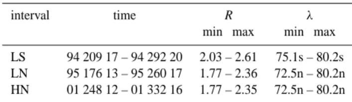
Table 1. The analysed data intervals: start and end times (year, day,

hour), minimum and maximum distances (R, in AU), and latitudes (λ, in degrees, with n and s for north and south, respectively).

interval time R λ

min max min max LS 94 209 17 – 94 292 20 2.03 – 2.61 75.1s – 80.2s LN 95 176 13 – 95 260 17 1.77 – 2.36 72.5n – 80.2n HN 01 248 12 – 01 332 16 1.77 – 2.35 72.5n – 80.2n

band, determined by the data sampling time (see above) and by the averaging time used to evaluate variances. Results dis-cussed here refer to hourly variances. This choice is based on the well-established result (e.g. see Tu and Marsch, 1995) that fluctuations on an hourly scale fall in the core of the in-ertial (f−5/3_{) Alfv´enic regime (see Goldstein et al., 1995,}

and Horbury et al., 1995). Shorter intervals would have too small a number of data points, while longer intervals would include contributions from low frequencies outside the iner-tial regime.

In addition to e+ and e−, two other quantities will be

used to describe Alfv´enic fluctuations, namely the normal-ized cross-helicity, σC, and the normalized residual energy,

σR (for a discussion on these quantities, see Matthaeus and

Goldstein, 1982, and Roberts et al., 1987a). They are defined as σC=(e+−e−)/(e++e−) and σR=(eV−eB)/(eV+eB), with

eV and eB the energies (per unit mass) of V and B/

√ 4πρ fluctuations, respectively, as given by their total variances (at hourly scale in the present case). Both parameters may only vary between −1 and +1. The cross-helicity σCgives a

mea-sure of the energy balance between the two components (out-ward and in(out-ward) of the Alfv´enic fluctuations. The value of σC is 1 (−1) when only the outward (inward) component is

present. Absolute values of σCbelow 1 correspond to a

mix-ture of the two components and/or to the presence of non-Alfv´enic variations in the solar wind parameters. The resid-ual energy σR gives the balance between kinetic and

mag-netic energy (with the magmag-netic field scaled to Alfv´en units through the factor 1/√4πρ). The absence of magnetic (ki-netic) fluctuations corresponds to σRequal to +1 (−1), while

equipartition gives σR=0. It should finally be recalled that

σC and σR have to fulfill the constraint σC2+σR2≤1

(pro-vided that σR6=±1, see Bavassano et al., 1998).

3 The investigated intervals and their Alfv´enic content

Our analysis is based on a comparison between fluctuations in post-maximum polar wind and in low-activity polar wind from the point of view of their Alfv´enic character. An in-spection of the post-maximum flows observed by Ulysses in the Northern Hemisphere during its second orbit (Fig. 2) has allowed one to identify at the highest latitudes an interval of three solar rotations (as seen by Ulysses) in which polar wind conditions appear to be well established. We have decided to

1516 B. Bavassano et al.: Alfv´enic fluctuations in “newborn” polar solar wind 400 600 800

1994

V

N

T

day

B

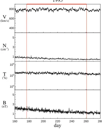
Fig. 3. Hourly averages of the solar wind velocity V , the proton

number density N , the proton temperature T , and the magnetic field magnitude B vs. time at the southern polar pass of the Ulysses first out-of-ecliptic orbit. Red lines indicate the interval that corresponds to the three southernmost solar rotations (label LS in Table 1).

study the Alfv´enic content of this interval and to compare it to that found for analogous (in terms of latitude and duration) intervals in low-activity polar wind.

The selected intervals are listed in Table 1, identified by a two-letter label (the first letter gives the solar activity level, L=low and H=high, the second letter is for the hemisphere, N=north and S=south). Intervals labeled LS and LN refer to the first Ulysses orbit, with LS for the southern polar cross-ing in 1994 and LN for the northern one in 1995, both at low solar activity. They have already been the object of past stud-ies on Alfv´enic fluctuations (e.g. see Goldstein et al., 1995; Smith et al. 1995; and Bavassano et al., 2000a, b). The third interval, labeled HN, is for the 2001 northern crossing at high solar activity. These intervals are highlighted as thick angu-lar sectors and dashed bands in Fig. 1 (LS and LN, around the South and North pole, respectively) and Fig. 2 (HN, around the North pole).

Hourly averages of the solar wind plasma (protons plus al-pha particles) velocity, the proton number density, the proton temperature, and the magnetic field magnitude for the inves-tigated intervals are shown in Figs. 3, 4, and 5 (between red lines). The 1994 and 1995 intervals correspond to very stable and almost identical wind conditions. The situation is not ex-actly the same for the newborn polar wind of the 2001 inter-val. Here, even though a fast wind appears well established

400 600 800

1995

V

N

T

day

B

Fig. 4. Solar wind parameters at the northern polar pass of the

Ulysses first out-of-ecliptic orbit, in the same format of Fig. 3. Red lines indicate the interval that corresponds to the three northernmost solar rotations (label LN in Table 1).

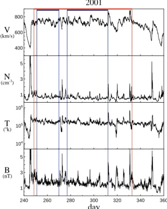
(see McComas et al., 2002), flow conditions are not as steady as for the 1994 and 1995 intervals, and several velocity gra-dients are observed. Though weak in comparison to those seen in low-latitude wind, these gradients represent non neg-ligible perturbations of the polar flow, with the development of compression/rarefaction regions. However, it clearly ap-pears from Fig. 5 that the 2001 sample has extended periods during which the wind is relatively steady (see blue lines).

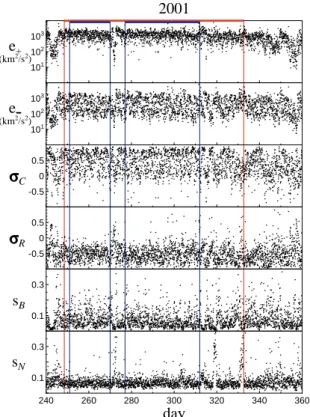
As discussed above, our analysis is based on the com-putation of hourly values of e+, e−, σC, and σR. In

addi-tion to this, to evaluate the level of variaaddi-tions of compressive type, hourly standard deviations of the magnetic field mag-nitude (sB) and the proton density (sN), normalized to B and

N hourly values, have been computed. Time plots of this set of parameters for the investigated intervals in 1994, 1995, and 2001 are shown in Figs. 6, 7, and 8, respectively.

The data shown in Figs. 6 and 7 are from the data set used by Bavassano et al. (2000a, b). As already well dis-cussed (see also Goldstein et al., 1995), these low-solar-activity polar samples are characterized by an Alfv´enic flow dominated by the outward fluctuations component, as easily seen from the displacement of σCtowards high positive

val-ues. Moreover, as is typical for observations outside ∼1 AU (e.g. see Matthaeus and Goldstein, 1982, and Roberts et al., 1987a), an imbalance of σR towards negative values (i.e.

400 600 800

2001

V

N

T

day

B

Fig. 5. Solar wind parameters at the northern polar pass of the

Ulysses second out-of-ecliptic orbit, in the same format of Fig. 3. Red lines indicate the three northernmost rotations interval (label HN in Table 1). Blue lines mark periods in which the wind is rela-tively steadier (see text).

to velocity fluctuations) is clearly apparent. All this occurs in the presence of low values of sBand sN, below 0.1 for the

large majority of cases.

Are these features observed in the 2001 newborn polar wind too? An answer can come from a comparison of Figs. 6 and 7 to Fig. 8, where the results for the 2001 interval are shown. As already mentioned above, flow conditions for this interval are less steady than for the 1994 and 1995 intervals, and this is expected to affect the Alfv´enic fluctuation prop-erties (e.g. see Roberts et al., 1987b, 1992). Velocity gra-dient effects are certainly present in the Fig. 8 data, with a decrease of σCand an increase of σR, sB, and sN. However,

if we focus on the intervals between blue lines, where (see above) the irregularities in the wind velocity are of lesser rel-evance, appreciable differences with respect to low-activity results (Figs. 6 and 7) do not come out. Thus, the Alfv´enic character appears to have been quickly recovered in the post-maximum polar wind.

4 The σC–σRand e+–e−pairs

To further compare the 2001 interval Alfv´enic features with those of the 1994 and 1995 intervals, an occurrence frequency analysis of the values of σC, σR, e+, and e−has

been performed. More specifically, 2-D histograms of the

101 102 103 1994 (kme2+_/s2₎ 101 102 103 (kme2_/s2₎ -0.5 0 0.5 C -0.5 0 0.5 R 0.1 0.3 sB 200 220 240 260 280 300 320 0.1 0.3 day sN

Fig. 6. From top to bottom, hourly values of e+, e−, σC, σR, sB,

and s_Nare plotted vs. time for the 1994 polar interval (LS).

parameter pairs σC–σR and e+–e− have been derived for

the three intervals. For 2001 data the analysis has been per-formed for both the whole interval and the subintervals de-limited by blue lines in Fig. 8. The histograms are shown as coloured contour plots in the panels of Figs. 9 and 10. A label in the upper left corner indicates the examined interval (2001∗is for the 2001 blue-line subintervals).

Histograms of Fig. 9 indicate that the Ulysses observations tend to cluster in the bottom right quadrant, where σCis

pos-itive and σRnegative. Following the constraint σC2+σR2≤1,

the σC–σRpairs fall inside a circle of radius 1, drawn in red

in the four panels (the small blue areas outside the circle are the effect of interpolations in constructing the coloured sur-face graphs). It is worth recalling (Bavassano et al., 1998) that the correlation coefficient between V and B/√4πρ fluc-tuations is closer to 1 (in absolute value) the closer to the unit circle the corresponding σC–σRpair falls.

A great similarity exists between the four distributions of Fig. 9. In all cases a prominent peak emerges at σC∼0.8

and σR∼−0.5, in the proximity of the unit circle (i.e. for

highly correlated velocity and magnetic fluctuations). It is accompanied by a tail extending towards σC∼0 and σR∼−1,

with a weak secondary peak at the end. The main peak is easily interpreted in terms of wind regions dominated by

Z+fluctuations. Not surprisingly, for the 2001∗ subset this

feature emerges in a cleaner way than for the whole 2001 sample. The secondary peak corresponds to cases for which magnetic fluctuations exist nearly in the absence of velocity

1518 B. Bavassano et al.: Alfv´enic fluctuations in “newborn” polar solar wind 101 102 103 1995 (kme2+_/s2₎ 101 102 103 (kme2_/s2₎ -0.5 0 0.5 C -0.5 0 0.5 R 0.1 0.3 sB 160 180 200 220 240 260 280 0.1 0.3 day sN

Fig. 7. Hourly values of e+, e−, σC, σR, sB, and sN vs. time for

the 1995 polar interval (LN).

fluctuations. Similar cases were observed in the inner helio-sphere by Tu and Marsch (1991), who interpreted them as a special type of convected magnetic structures. Thus, his-tograms of Fig. 9 indicate that the polar wind fluctuations es-sentially are a mixture of Alfv´enic fluctuations and convected structures of magnetic type (see also Bavassano et al., 1998). This is a support to models (e.g. Tu and Marsch, 1993) based on a superposition of such two components.

The frequency distributions shown in Fig. 10 indicate that also for the Z+ and Z− fluctuation energies essentially the

same pattern is observed in the different samples. The great majority of points falls within a narrow band close to the e+=10e− line (white solid line). The e+–e− pairs of this

band represent the Alfv´enic population typically found in the polar wind, with a largely dominant contribution from outgoing fluctuations, and correspond to the main peak at σC∼0.8 seen in Fig. 9 (σC is 0.82 for e+/e−=10). The

re-maining points mostly fall in the region between the band and the e+=e−line (white dashed line). As is obvious, the

e+∼e− cases of Fig. 10 correspond to the σC∼0 cases of

Fig. 9. It is worth mentioning that the e+values in the main

band tend to be higher for the 1995 interval. This could be an effect of the lower level of variability that characterizes the wind seen by Ulysses during the northern polar pass in 1995, as compared to other polar wind phases (e.g. see Bavassano et al., 2005). 101 102 103 2001 (kme2+_/s2₎ 101 102 103 (kme2_/s2₎ -0.5 0 0.5 C -0.5 0 0.5 R 0.1 0.3 sB 240 260 280 300 320 340 360 0.1 0.3 day sN

Fig. 8. Hourly values of e+, e−, σC, σR, sB, and sNvs. time for the

2001 polar interval (HN). Blue lines mark wind regions relatively unaffected by velocity gradient effects.

5 Summary and conclusion

The dependence of the 3-D structure of the solar wind on the Sun’s activity cycle, first seen in wind speed values esti-mated from interplanetary scintillation, has been unambigu-ously confirmed by in-situ measurements of Ulysses, the first spacecraft able to perform an almost complete latitu-dinal scan of the heliosphere. At low solar activity a bi-modal structure is dominant, with a fast and uniform flow at high latitudes, and slow and variable flows at low latitudes. Around solar maximum, in sharp contrast, variable flows are observed at all latitudes. This last kind of pattern, however, has a relatively short life. In fact, quite soon after solar max-imum the fast high-latitude wind is seen to regain its role, though solar activity remains high (see Fig. 2).

From statistical distributions of the Ulysses measurements McComas et al. (2002) have concluded that the 2001 new-born polar flows exhibit plasma features (as velocity, den-sity, temperature, and alpha-particle abundance) virtually in-distinguishable from those typical of the low-solar-activity polar wind. However, when time profiles of wind velocity, density, temperature, and magnetic field are examined for the intervals investigated here (see Figs. 3 to 5), flow conditions in 2001 do not appear to be as steady as in 1994 and 1995. Though weak in comparison to gradients seen in low-latitude wind, the velocity variations observed in the 2001 sample represent non negligible perturbations in the plasma flow,

-1 -0.5 0 0.5 R P(%) 0 1 2 3 4 5 6

1994

1995

2001

2001

Fig. 9. Occurrence frequency distributions of the σ_C-σ_Rpairs are shown in the four panels, with the label in the upper left corner to indicate the interval under examination. The 2001∗panel is for the subintervals of the 2001 sample (highlighted by the blue lines in Figs. 5 and 8). The colour code for the occurrence frequency P (in per cent) is shown on top. The red circle indicates the limit value for the sum of σC2and σR2(see text).

with clear evidence of compression and rarefaction effects. The point addressed in the present paper is about a relevant feature of the low-activity polar wind, namely the ubiquitous presence of a strong flow of Alfv´enic fluctuations. Does this remain valid for the post-maximum polar wind too?

In order to obtain an answer to this question we have deter-mined for the post-maximum polar flow seen in 2001 the val-ues of the parameters that are generally used to characterize fluctuations of Alfv´enic type (namely Z+and Z−fluctuation

energies, normalized cross-helicity, and normalized residual energy) and have compared them with those obtained for low-activity polar wind intervals in 1994 and 1995 (already investigated by Bavassano et al., 2000a, b). From this com-parison (e.g. see Figs. 9 and 10) it clearly appears that sig-nificant differences between the examined samples for the values of e+, e−, σC, and σRdo not come out. Thus, though

the plasma flow for the post-maximum polar interval is not as steady as for those at low solar activity, the Alfv´enic char-acter of the fluctuations clearly appears to be essentially the same.

In conclusion, the main features of the flow of Alfv´enic fluctuations typical of the low-activity polar wind are fully recovered in the newborn polar streams seen shortly after the solar maximum. 0 500 1000 1500 2000 (km2 /s2 )

e

1994

1995

e

e

2001

e

2001

Fig. 10. Fluctuation energies are shown in terms of occurrence

fre-quency distributions in the e+–e−plane. The four panels have the

same meaning as in Fig. 9. The colour code for the occurrence frequency P (in per cent) is shown on top. White lines are for e+=10e−(solid) and e+=e−(dashed).

Acknowledgements. The use of data of the plasma analyzer

(princi-pal investigator D. J. McComas, Southwest Research Institute, San Antonio, Texas, USA) and of the magnetometers (principal investi-gator A. Balogh, The Blackett Laboratory, Imperial College, Lon-don, UK) aboard the Ulysses spacecraft is gratefully acknowledged. The data have been made available through the World Data Center A for Rockets and Satellites (NASA/GSFC, Greenbelt, Maryland, USA). Solar sunspot data are from the World Data Center for the Sunspot Index, Royal Observatory of Belgium (Brussels, Belgium). Topical Editor R. Forsyth thanks M. L. Goldstein and another referee for their help in evaluating this paper.

References

Balogh, A., Forsyth, R. J., Lucek, E. A., and Horbury, T. S.: He-liospheric magnetic field polarity inversions at high heliographic latitudes, Geophys. Res. Lett., 26, 631–634, 1999.

Bavassano, B., Bruno, R., and Carbone, V.: MHD Turbulence in the Heliosphere, in: The Sun and the heliosphere as an integrated system, edited by Poletto, G. and Suess, S. T., Kluwer Academic Publishers, Dordrecht, The Netherlands, Astrophysics and Space Science Library, v. 317, 253–281, 2004.

Bavassano, B., Bruno, R., and D’Amicis, R.: Large-scale velocity fluctuations in polar solar wind, Ann. Geophys., 23, 1025-1031, 2005, SRef-ID: 1432-0576/ag/2005-23-1025.

1520 B. Bavassano et al.: Alfv´enic fluctuations in “newborn” polar solar wind Bavassano, B., Pietropaolo, E., and Bruno, R.: Cross-helicity and

residual energy in solar wind turbulence: radial evolution and latitudinal dependence in the region from 1 to 5 AU, J. Geophys. Res., 103, 6521–6529, 1998.

Bavassano, B., Pietropaolo, E., and Bruno, R.: Alfv´enic turbu-lence in the polar wind: A statistical study on cross helicity and residual energy variations, J. Geophys. Res., 105, 12 697–12 704, 2000a.

Bavassano, B., Pietropaolo, E., and Bruno, R.: On the evolution of outward and inward Alfv´enic fluctuations in the polar wind, J. Geophys. Res., 105, 15 959–15 964, 2000b.

Dobrowolny, M., Mangeney, A., and Veltri, P.: Properties of mag-netohydrodynamic turbulence in the solar wind, Astron. Astro-phys., 83, 26–32, 1980.

Els¨asser, W. M.: The hydromagnetic equations, Phys. Rev., 79, 183–183, 1950.

Goldstein, B. E., Smith, E. J., Balogh, A., Horbury, T. S., Goldstein, M. L., and Roberts, D. A.: Properties of magnetohydrodynamic turbulence in the solar wind as observed by Ulysses at high heli-ographic latitudes, Geophys. Res. Lett., 22, 3393–3396, 1995. Horbury, T. S., Balogh, A., Forsyth, R. J., and Smith, E. J.:

Obser-vations of evolving turbulence in the polar solar wind, Geophys. Res. Lett., 22, 3401–3404, 1995.

Horbury, T. S. and Tsurutani, B. T.: Ulysses measurements of waves, turbulence and discontinuities, in: The heliosphere near solar minimum: The Ulysses perspective, edited by: Balogh, A., Marsden, R. G., and Smith, E. J., Springer-Praxis Books in As-trophysics and Astronomy, London, UK, ISBN 1-85233-204-2, 167–227, 2001.

Jones, G. H., Balogh, A., and Smith, E. J.: Solar magnetic field reversal as seen at Ulysses, Geophys. Res. Lett., 30(19), 8028, doi:10.1029/2003GL017204, 2003.

Matthaeus, W. H. and Goldstein, M. L.: Measurement of the rugged invariants of magnetohydrodynamic turbulence in the solar wind, J. Geophys. Res., 87, 6011–6028, 1982.

McComas, D. J., Bame, S. J., Barraclough, B. L., Feldman, W. C., Funsten, H. O., Gosling, J. T., Riley, P., Skoug, R., Balogh, A., Forsyth, R., Goldstein, B. E., and Neugebauer, M.: Ulysses re-turn to the slow solar wind, Geophys. Res. Lett., 25, 1–4, 1998. McComas, D. J., Barraclough, B. L., Funsten, H. O., Gosling, J.

T., Santiago-Mu˜noz, E., Skoug, R. M., Goldstein, B. E., Neuge-bauer, M., Riley, P., and Balogh, A.: Solar wind observations over Ulysses first full polar orbit, J. Geophys. Res., 105, 10 419– 10 433, 2000.

McComas, D. J., Elliot, H. A., Gosling, J. T., Reisenfeld, D. B., Skoug, R. M., Goldstein, B. E., Neugebauer, M., and Balogh, A.: Ulysses’ second fast-latitude scan: Complexity near solar maximum and the reformation of polar coronal holes, Geophys. Res. Lett., 29(9), doi:10.1029/2001GL014164, 2002.

McComas, D. J., Elliott, H. A., Schwadron, N. A., Gosling, J. T., Skoug, R. M., and Goldstein, B. E.: The three-dimensional solar wind around solar maximum, Geophys. Res. Lett., 30(10), 1517, doi:10.1029/2003GL017136, 2003.

Miralles, M. P., Cranmer, S. R., and Kohl, J. L.: UVCS observations of a high-latitude coronal hole with high oxygen temperatures and the next solar cycle polarity, Ap. J., 560, L193–L196, 2001. Rickett, B. J. and Coles, W. A.: Solar cycle evolution of the solar wind in three dimensions, Proceedings of Solar Wind 5 Confer-ence, edited by: Neugebauer, M., NASA Conference Publication 2280, 315–321, 1983.

Roberts, D. A., Klein, L. W., Goldstein, M. L., and Matthaeus, W. H.: The nature and evolution of magnetohydrodynamic fluctua-tions in the solar wind: Voyager observafluctua-tions, J. Geophys. Res., 92, 11 021–11 040, 1987a.

Roberts, D. A., Goldstein, M. L., Klein, L. W., and Matthaeus, W. H.: Origin and evolution of fluctuations in the solar wind: Helios observations and Helios-Voyager comparisons, J. Geophys. Res., 92, 12 023–12 035, 1987b.

Roberts, D. A., Goldstein, M. L., Matthaeus, W. H., and Ghosh, S.: Velocity shear generation of solar wind turbulence, J. Geophys. Res., 97, 17 115–17 130, 1992.

Smith, E. J., Balogh, A., Neugebauer, M., and McComas, D. J.: Ulysses observations of Alfv´en waves in the southern and north-ern solar hemispheres, Geophys. Res. Lett., 22, 3381–3384, 1995.

Tu, C.-Y. and Marsch, E.: A case study of very low cross-helicity fluctuations in the solar wind, Ann. Geophys., 9, 319–332, 1991. Tu, C.-Y. and Marsch, E.: A model of solar wind fluctuations with two components: Alfv´en waves and convective structures, J. Geophys. Res., 98, 1257–1276, 1993.

Tu, C.-Y. and Marsch, E.: MHD structures, waves and turbulence in the solar wind: Observations and theories, Space Sci. Rev., 73, 1–210, 1995.