HAL Id: inserm-00663766
https://www.hal.inserm.fr/inserm-00663766
Submitted on 27 Jan 2012
HAL is a multi-disciplinary open access
archive for the deposit and dissemination of
sci-entific research documents, whether they are
pub-lished or not. The documents may come from
teaching and research institutions in France or
abroad, or from public or private research centers.
L’archive ouverte pluridisciplinaire HAL, est
destinée au dépôt et à la diffusion de documents
scientifiques de niveau recherche, publiés ou non,
émanant des établissements d’enseignement et de
recherche français ou étrangers, des laboratoires
publics ou privés.
factor study in breast cancer.
Carine Bellera, Gaëtan Macgrogan, Marc Debled, Christine de Lara,
Véronique Brouste, Simone Mathoulin-Pélissier
To cite this version:
Carine Bellera, Gaëtan Macgrogan, Marc Debled, Christine de Lara, Véronique Brouste, et al..
Vari-ables with time-varying effects and the Cox model: some statistical concepts illustrated with a
prog-nostic factor study in breast cancer.. BMC Medical Research Methodology, BioMed Central, 2010,
10 (1), pp.20. �10.1186/1471-2288-10-20�. �inserm-00663766�
R E S E A R C H A R T I C L E
Open Access
Variables with time-varying effects and the Cox
model: Some statistical concepts illustrated with
a prognostic factor study in breast cancer
Carine A Bellera
1,5*, Gaëtan MacGrogan
2, Marc Debled
3, Christine Tunon de Lara
4, Véronique Brouste
1,
Simone Mathoulin-Pélissier
1,5Abstract
Background: The Cox model relies on the proportional hazards (PH) assumption, implying that the factors investigated have a constant impact on the hazard - or risk - over time. We emphasize the importance of this assumption and the misleading conclusions that can be inferred if it is violated; this is particularly essential in the presence of long follow-ups.
Methods: We illustrate our discussion by analyzing prognostic factors of metastases in 979 women treated for breast cancer with surgery. Age, tumour size and grade, lymph node involvement, peritumoral vascular invasion (PVI), status of hormone receptors (HRec), Her2, and Mib1 were considered.
Results: Median follow-up was 14 years; 264 women developed metastases. The conventional Cox model
suggested that all factors but HRec, Her2, and Mib1 status were strong prognostic factors of metastases. Additional tests indicated that the PH assumption was not satisfied for some variables of the model. Tumour grade had a significant time-varying effect, but although its effect diminished over time, it remained strong. Interestingly, while the conventional Cox model did not show any significant effect of the HRec status, tests provided strong evidence that this variable had a non-constant effect over time. Negative HRec status increased the risk of metastases early but became protective thereafter. This reversal of effect may explain non-significant hazard ratios provided by previous conventional Cox analyses in studies with long follow-ups.
Conclusions: Investigating time-varying effects should be an integral part of Cox survival analyses. Detecting and accounting for time-varying effects provide insights on some specific time patterns, and on valuable biological information that could be missed otherwise.
Background
Survival analysis, or time-to-event data analysis, is widely used in oncology since we are often interested in studying a delay, such as the time from cancer diagnosis or treatment initiation to cancer recurrence or death. Thanks to the improvement of cancer treatments, and the induced longer life expectancy, we observe an increasing number of studies with long follow-up peri-ods. Statistical models to analyze such data should thus adequately account for the increasing duration of fol-low-ups. The Cox proportional hazards (PH) model
allows one to describe the survival time as a function of multiple prognostic factors [1]. This model relies on a fundamental assumption, the proportionality of the hazards, implying that the factors investigated have a constant impact on the hazard - or risk - over time. If time-dependent variables are included without appropri-ate modeling, the PH assumption is violappropri-ated. As a result, misleading effect estimates can be derived, and signifi-cant effect in the early (or late) follow-up period may be missed. Checking the proportionality of the hazards should thus be an integral part of a survival analysis by a Cox model. The assumption, however, is not systema-tically verified. In a 1995 review of cancer publications using a Cox model, Altman et al. reported that most
* Correspondence: bellera@bergonie.org
1Department of Clinical Epidemiology and Clinical Research, Institut Bergonié, Regional Comprehensive Cancer Centre, Bordeaux, France
© 2010 Bellera et al; licensee BioMed Central Ltd. This is an Open Access article distributed under the terms of the Creative Commons Attribution License (http://creativecommons.org/licenses/by/2.0), which permits unrestricted use, distribution, and reproduction in any medium, provided the original work is properly cited.
studies did not report verifying this assumption [2]; similar findings were reported recently by one of the co-authors of the present work [3].
Although the Cox model has been widely used (more than 25 000 citations since the publication of the origi-nal paper by Cox [4]), recent publications suggest a growing interest in the quality of its applications. Special papers in statistics have been published in the oncology literature providing general introductions to survival analysis [5-8]; topics covered included summarizing sur-vival data, testing for a difference between groups, pre-senting existing statistical models, or assessing the adequacy of a survival model. Others works focused on providing definition of specific survival endpoints [9], or on the quality of reporting of survival events [3].
Assessing whether the assumption of proportional hazards is a central theme in survival analysis, and as such is discussed in several statistical textbooks [10-14] as well as in the general statistical literature [15-18]. To our knowledge however, this topic has been discussed in few medical journals. Importantly, this strong assump-tion does not seem to be systematically assessed. For illustration, a recent review of clinical trials with primary analyses based on survival end points showed that only one of the 64 papers that used a Cox model mentioned verifying the PH assumption [3].
Our objective is to inform clinicians, as well as those who read and write manuscripts in medical journals, about the importance of the underlying PH assumption, the misleading conclusions that can be inferred if it is violated, as well as the additional information provided by verifying it. After a theoretical introduction, we describe techniques to assess if this assumption is vio-lated, and model strategies to account for, and describe time-dependency. We illustrate our discussion with a study on prognostic factors in breast cancer.
Methods and results
Survival analysis
In many studies, the primary variable of interest is a delay, such as the time from cancer diagnosis to a parti-cular event of interest. This event may be death, and for this reason the analysis of such data is often referred to as survival analysis. The event of interest may not have occurred at the time of the statistical analysis, and simi-larly, a subject may be lost to follow-up before the event is observed. In such case, data are said to be censored at the time of the analysis or at the time the patient was lost to follow-up. Censored data still bring some infor-mation since although we do not know the exact date of the event, we know that it occurred later than the cen-soring time.
Both the Kaplan-Meier method and the Cox propor-tional hazards (PH) model allow one to analyze
censored data [1,19], and to estimate the survival prob-ability, S(t), that is the probability that a subject survives beyond some time t. Statistically, this probability is pro-vided by the survival function S(t) = P (T > t), where T is the survival time. The Kaplan Meier method estimates the survival probability non-parametrically, that is, assuming no specific underlying function [19]. Several tests are available to compare the survival distributions across groups, including the log-rank and the Mann-Whitney-Wilcoxon tests [20,21]. The Cox PH model accounts for multiple risk factors simultaneously. It does not posit any distribution, or shape for the survival function, however, the instantaneous incidence rate of the event is modeled as a function of time and risk factors.
The instantaneous hazard rate at time t, also called instantaneous incidence, death, or failure rate, or risk, is the instantaneous probability of experiencing an event at time t, given that the event has not occurred yet. It is a rate of event per unit of time, and is allowed to vary over time. Just as the risk of events per unit time, one can make an analogy by considering the speed given by a car speedometer, which represents the distance tra-velled per unit of time. Suppose, that the event of inter-est is death, and we are interinter-ested in its association with n covariates, X1, X2, ..., Xn, then the hazard is given by:
h tx( )h t0( ) exp(1 1x 2 2x n nx ) (1) The baseline hazard rate h0(t) is an unspecified non-negative function of time. It is the time-dependent part of the hazard and corresponds to the hazard rate when all covariate values are equal to zero. b1, b2, ..., bn are the coefficients of the regression function b1x1+ b2x2+... bnxn. Suppose that we are interested in a single covariate then the hazard is:
h tx( )h t0( ) exp(x) (2) The hazards for two subjects with covariate values x1 and x2 are thus given respectively by hx1(t) = h0(t) exp (bx1) and hx2(t) = h0(t) exp(bx2), and the hazard ratio is expressed as:
HRhx2( ) /t hx1( )t exp[ ( x2x1)] (3)
Taking x2 = x1 + 1, the hazard ratio reduces to HR = exp(b) and corresponds to the effect of one unit increase in the explanatory variable X on the risk of event. Since b = log(HR), b is referred as the log hazard ratio. Although the hazard rate hx(t) is allowed to vary over time, the hazard ratio HR is constant; this is the assumption of proportional hazards. If the HR is greater than 1 (b > 0), the event risk is increased for subjects with covariate value x2 compared to subjects with
covariate value x1, while a HR lower than 1 (b < 0) indi-cates a decreased risk. When the HR is not constant over time, the variable is said to have a time-varying effect; for example, the effect of a treatment can be strong immediately after treatment but fades with time. This should not be confused with a time-varying covari-ate, which is a variable whose value is not fixed over time, such as smoking status. Indeed, a person can be a non-smoker, then a smoker, then a non-smoker. Note however, that a variable may be both time-varying and have an effect that changes over time.
In a Cox PH model, the HR is estimated by consider-ing each time t at which an event occurs. When esti-mating the overall HR over the complete follow-up period, the same weights are given to the very early HR which affect almost all individuals and to very late HR affecting only the very few individuals still at risk. The HR is thus averaged over the event times. In the case of proportional hazards, the overall HR is not affected by this weighting procedure. If, on the other hand, the HR changes over time, that is, the hazard rates are not pro-portional, then equal weighting may result in a non-representative HR, and may produce biased results [22]. It should be noted that the HR is averaged over the event times rather than over the follow-up time. It is unchanged if the time scale is changed without disturb-ing the orderdisturb-ing of events.
Example
We applied some of the presented methods to breast cancer patients as time-varying effects have been reported, such as for nodal or hormone receptor status, [23-26]. We studied women with non-metastatic, oper-able breast cancer who underwent surgery between 1989 and 1993 at our institution, and who did not receive previous neoadjuvant treatment. Exclusion criteria included a previous history of breast carcinoma, concur-rent contralateral breast cancer, and pathologic data missing. Follow-up was performed according to the Eur-opean Good Clinical Practice requirements and con-sisted of regular physical examinations, and annual X-ray mammogram, and additional assessments in case of suspected metastases. Clinical and pathological charac-teristics were analyzed according to the hospital-recorded file at the time of treatment initiation. Patholo-gical tumour size (≤ or > 20 mm) was measured on fresh surgical specimens. A modified version of the Scarff-Bloom-Richardson grading system was used (SBR grade I, II, or III). PVI (Yes, No) was defined as the pre-sence of neoplastic emboli within unequivocal vascular lymphatic or capillary lumina in areas adjacent to the breast tumour. Exploratory immuno-histochemical ana-lyses were performed on a tissue microarray (TMA) to assess hormone receptor (HRec) status (positive if
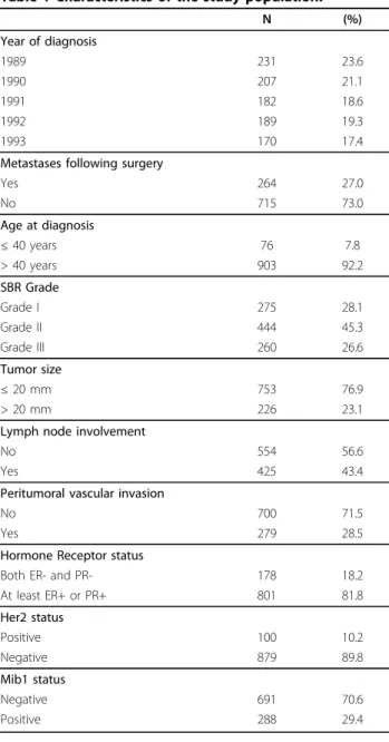
ER-positive and/or progesterone receptor [PgR]-ER-positive). ER and PgR expression levels were evaluated semi-quan-titatively according to a standard protocol with cut-off values at 10% positive tumor cells. Her2 expression level was evaluated according to the Herceptest scoring sys-tem [27]. Mib1 expression level was evaluated semi-quantitatively. Information on all factors was available for 979 women (Table 1). The median follow-up time was 14 years (95% confidence interval: 13.7 - 14.2) and 264 women developed metastases.
Working example
The prognostic factors were initially selected based on current knowledge regarding risk of metastases. They were next analyzed using a conventional Cox regression model; all were statistically significant at the 5% level in
Table 1 Characteristics of the study population.
N (%) Year of diagnosis 1989 231 23.6 1990 207 21.1 1991 182 18.6 1992 189 19.3 1993 170 17.4
Metastases following surgery
Yes 264 27.0 No 715 73.0 Age at diagnosis ≤ 40 years 76 7.8 > 40 years 903 92.2 SBR Grade Grade I 275 28.1 Grade II 444 45.3 Grade III 260 26.6 Tumor size ≤ 20 mm 753 76.9 > 20 mm 226 23.1
Lymph node involvement
No 554 56.6
Yes 425 43.4
Peritumoral vascular invasion
No 700 71.5
Yes 279 28.5
Hormone Receptor status
Both ER- and PR- 178 18.2
At least ER+ or PR+ 801 81.8 Her2 status Positive 100 10.2 Negative 879 89.8 Mib1 status Negative 691 70.6 Positive 288 29.4
the univariate analyses, and were then entered onto a multivariate Cox model. The risk of metastases was increased for women with younger age compared to older age; grade II and III tumours compared to grade I tumours; large compared to small tumour sizes; lymph node involvement compared to no involvement; and PVI compared to no PVI (Additional file 1: Estimated log hazard ratios (log(HR)), and hazard ratios (HR = exp ( ˆ )) with 95% confidence intervals (95% CI) and p-values for model covariates when fitting a multivariate conventional Cox model and a Cox model with time-by-covariate interactions.). Based on this model, all vari-ables, but hormone receptor, Her2 and Mib1 status, sig-nificantly affected the risk of metastases.
Assessing non-proportionality: Graphical strategy
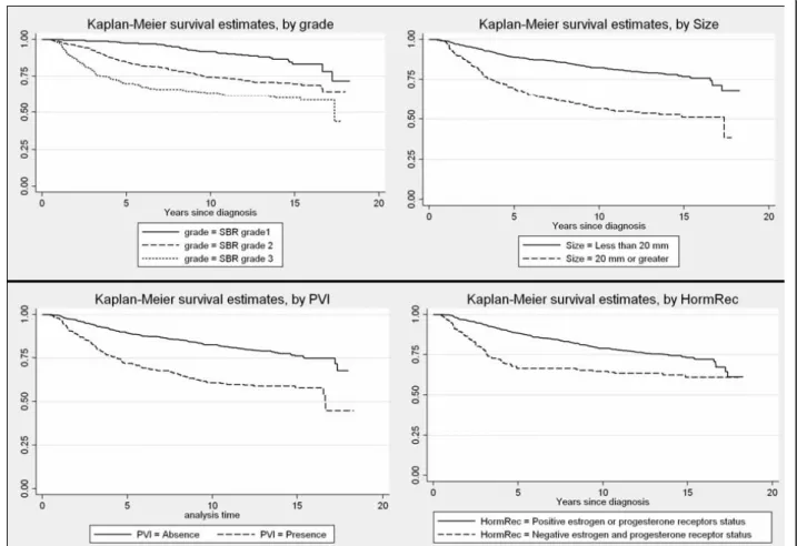
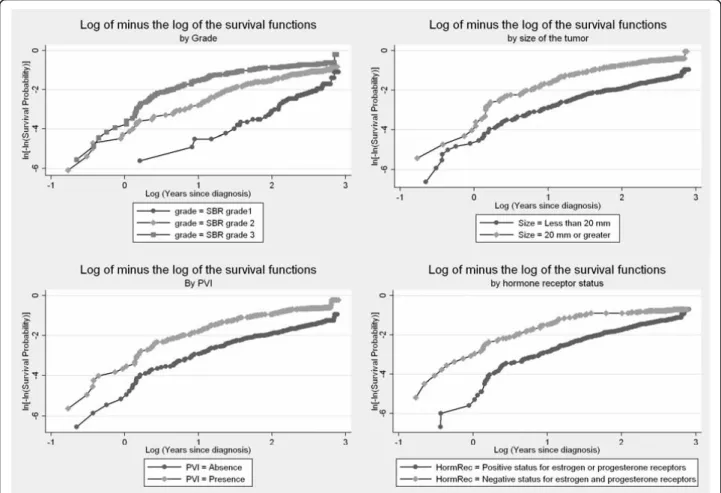
In the presence of a categorical variable, one can plot the Kaplan-Meier survival distribution, S(t), as a func-tion of the survival time, for each level of the covariate. If the PH assumption is satisfied, the curves should stea-dily drift apart. One can also apply a transformation of the Kaplan-Meier survival curves and plot the function log(-log(S(t))) as a function of the log survival time, where log represents the natural logarithm function. If the hazards are proportional, the stratum specific log-minus-log plots should exhibit constant differences, that is be approximately parallel. These visual methods are simple to implement but have limitations. When the covariate has more than two levels, Kaplan-Meier plots are not useful for discerning non-proportionality because the graphs become to cluttered [10]. Similarly, although the PH assumption may not be violated, the log-minus-log curves are rarely perfectly parallel in prac-tice, and tend to become sparse at longer time points, and thus less precise. It is not possible to quantify how close to parallel is close enough, and thus how propor-tional the hazards are. The decision to accept the PH hypothesis often depends on whether these curves cross each other. As a result, the decision to accept the PH hypothesis can be subjective and conservative [28], since one must have strong evidence (crossing lines) to con-clude that the PH assumption is violated. In view of these limitations, some suggest providing standard
errors to these plots [29]. This approach however can be computationally intensive and is not directly available in standard computer programs. Kaplan-Meier and log-minus-log plots are available from most standard statis-tical packages (Table 2).
Working example (cont’)
Kaplan-Meier survival curves and log-minus-log plots are shown for some variables (Figures 1 and 2). The Kaplan-Meier survival curves appeared to steadily drift apart for all but the hormone receptor status, Her2 sta-tus, and mib1 status. The log-minus log plots looked approximately parallel for Age, size of the tumour, lymph node involvement, and PVI. Again, plots for the hormone receptor status, Her2 status, and mib1 status tended to indicate a violation of the PH assumption. There was also some suspicion with respect to the SBR grade.
Assessing non-proportionality: Modelling and testing strategies
Graphical methods for checking the PH assumption do not provide a formal diagnostic test, and confirmatory approaches are required. Multiple options for testing and accounting for non-proportionality are available.
Cox proposed assessing departure from non-propor-tionality by introducing a constructed time-dependent variable, that is, adding an interaction term that involves time to the Cox model, and test for its significance [1]. Suppose one is interested in evaluating if some variable X has a time-varying effect. A time-dependent variable is created by forming an interaction (product) term between the predictor, X (continuous or categorical), and a function of time t (f(t) = t, t2, log(t), ...). Adding this interaction to the model (equation 2), the hazard then becomes:
h tx( )h t0( ) exp[x. . ( )]x f t (5) The hazard ratio is given by HR(t) = hx+1(t)/hx(t) = exp[b + g.x.f(t)] for a unit increase in the variable X, and is time-dependent through the function f(t). If g > 0 (g < 0), then the HR increases (decreases) over time. Testing for non-proportionality of the hazards is
Table 2 Statistical software
R/Splus© SAS© SPSS© Stata©
Graphical checks survfit function lifetest procedure Survt command sts command
Time-by-covariate interactions
programming required. phreg procedure (definition of interactions)/test statement.
time program command (definition of interactions)/cox reg command.
tvc option/stcox command Scaled Schonfeld
residuals
cox.zph function phreg procedure/ressch option Not directly available/programming required stphtest command Cumulative residuals Timereg/gof libraries/ cum.residuals function phreg procedure/assess statement/ph option
Not directly available/programming required
Not directly available/ programming required
equivalent to testing if g is significantly different from zero. One can use different time functions such as poly-nomial or exponential decay but often very simple fixed functions of time such as linear or logarithmic functions are preferred [28]. This modeling approach also provides estimates of the hazard ratio at different time points since values t of time can be fitted into the hazard ratio function. Time-dependent variables provide a flexible method to evaluate departure from non-proportionality and an approach to building a model for the depen-dence of relative risk over time. This approach however should be used with caution. Indeed, if the function of time selected is mis-specified, the final model will not be appropriate. This is a disadvantage of this method over more flexible approach.
Working example (cont’)
We created time-by-covariate interactions for each vari-able of the model, by introducing products between the variables and a linear function of time. As shown in Additional File 1 (Estimated log hazard ratios (log(HR)), and hazard ratios (HR = exp( ˆ )) with 95% confidence intervals (95% CI) and p-values for model covariates
when fitting a multivariate conventional Cox model and a Cox model with time-by-covariate interactions.), sig-nificant time-by-covariate interactions involved the SBR grade, hormone receptor status, Her2 status, and PVI (p < 0.05). Thus these results indicated that the hazard ratios associated with these factors were not constant over time. The parameters ( ˆ ) associated with most interactions were negative, suggesting that the hazard ratios were decreasing over time. The estimated hazard ratio associated with an SBR grade II (versus grade I) as a function of time t was given by: HR(t) = exp(1.71 -0.14t). Hazard ratios were 4.8, 3.6, and 2.7 at respec-tively 1, 3, and 5 years. Similarly, the estimated hazard ratio associated with the hormone receptor status was: HR(t) = exp(0.73 - 0.14t), that is hazard ratios of 1.8, 1.3, and 1.0 at respectively 1, 3, and 5 years. While the conventional Cox model did not show any significant effect for hormone receptors, Her2 and Mib1, these variables had a significant effect once time-by-covariate interactions were included.
Departure from non-proportionality can also be inves-tigated using the residuals of the model. A residual
measures the difference between the observed data, and the expected data under the assumption of the model. Schoenfeld residuals are calculated and reported at every failure time under the PH assumption, and as such are not defined for censored subjects [15,30]. They are defined as the covariate value for the individual that failed minus its expected value assuming the hypotheses of the model hold. There is a separate residual for each individual for each covariate. A smooth plot of the Schoenfeld residuals can then be used to directly visua-lize the log hazard ratio [15]. Assuming proportionality of the hazards, the Schoenfeld residuals are independent of time. Thus, a plot suggesting a non-random pattern against time is evidence of non-proportionality. Graphi-cally, this method is more reliable and easier to interpret than plotting the log(-log(S(t)) function presented ear-lier. The presence of a linear relationship with time can be tested by performing a simple linear regression and a test trend. A slope significantly different from zero would be evidence against proportionality: an increasing (decreasing) trend would indicate an increasing (decreasing) hazard ratio over time. It is recommended to carefully look at the residual plot in addition to
performing this test as some patterns may be apparent on the plots (quadratic, logarithmic), but remain unde-tected by the statistical test. Moreover, undue influence of outliers might become obvious [10]. Although, the method based on the smoothed Schoenfeld residuals provides time-dependent estimates, it can have some drawbacks [14,18]. The uncertainty estimates associated with the resulting time-dependent estimates can be diffi-cult to use in practice, and the estimator provided may not have good statistical properties, such as consistency. Importantly, p-values resulting from trend tests based on the Schoenfeld residuals are obtained independently for each covariate of the model, assuming the Cox model is justified for the other covariates of the model; as such, results should be interpreted carefully. Tests based on the Schoenfeld residuals can be easily imple-mented in most standard statistical packages (Table 2).
Working example (cont’)
For each covariate, scaled Schoenfeld residuals were plotted over time, and tests for a zero slope were per-formed. The corresponding values, as well as the p-value associated with a global test of non-proportionality are reported in Table 3. The global test suggested strong
evidence of non-proportionality (p < 0.01). Variables that deemed most likely to contribute to non-propor-tionality were the SBR grade (p < 0.01), PVI (p = 0.05) and hormone receptor status (p = 0.05). These numeri-cal findings suggest a non constant hazard ratio for these variables. Residuals help visualizing the log hazard ratio ˆ over time for each covariate (figure 3). We added dashed and dotted lines representing respectively the null effect (null log hazard ratio) and the averaged log hazard ratio estimated by the conventional Cox model. With respect to the SBR grade, the plots sug-gested strong effect over the first five years. This effect tended to diminish afterwards. Similarly, the impact of PVI changed over time, with again higher risks of metastases in the early years, and then this effect tended to vanish. Concerning hormone receptor status, plots suggested that a negative status increased the risk of metastases early on, and became protective afterwards.
The cumulative sum of Schoenfeld residuals, or equivalently the observed score process can also be used to assess proportional hazards [31]. Graphically, the observed score process is plotted versus time for each variable of the model, together with simulated processes assuming the underlying Cox model is true, that is, assuming proportional hazards. Any departure of the observed score process from the simulated ones is evi-dence against proportionality. These plots can then be used to assess when the lack of fit is present. In particu-lar, an observed score well above the simulated process is an indication of an effect higher than the average one, and conversely. This method is particularly well illu-strated in a recent publication by Cortese et al. [18]. Goodness-of-fit tests can be implemented based on the cumulative residuals. The cumulative residuals based approach overcomes some drawbacks encountered with the Schoenfeld residuals, since resulting estimators tend to have better statistical properties, and justified p-values are derived [14]. The cumulative residuals
approach is implemented in some standard statistical packages (Table 2).
Working example (cont’)
Tests based on cumulative residuals are presented in Table 4. At the 5% significance level, test statistics sug-gest non-constant effect over time for the grade of the tumor, as well as the status of the hormone receptors, her2, and Mib1. For illustration, we also plotted the resulting score process for some variables (Figure 4). In accordance with the test statistics based on the cumula-tive residuals, we observe strong departure of the observed processes from the simulated curves under the model for the grade and hormone receptor status. These plots are particularly useful in identifying where the lack of fit is present. For example, the initial positive score process associated with hormone receptors, suggests that the effect of this variable is initially higher than the average effect, and thus lower than the average effect afterwards. That is, the risk of metastases is increased initially for women with both negative hormone recep-tors compared to the average risk, and decreased afterwards.
Another simple approach for testing time-varying effects of covariates involves fitting different Cox models for different time periods. Indeed, although the PH assumption may not hold over the complete follow-up period, it may hold over a shorter time window. Unless there is an interest in a particular cut-off time value, two subsets of data can be created based on the median event time [10]. That is, a first analysis is conducted by censoring everyone still at risk beyond this time point, and a second one by considering only those subjects still at risk thereafter. In such case, the interpretation of the models is conditional on the length of the survival time, and results should thus be interpreted with cau-tion. Even if the period of analysis is shortened, one should still ensure that the PH assumption is not vio-lated within these reduced time periods. Moreover, since fewer event times are considered, analyses can suf-fer from a decreased power. Finally, although this method is particularly simple to implement and might provide sufficient information in some settings, that is if one is interested in a short time window, it should be noted that this method is not directly testing the PH assumption, and a different parametrization would be needed to perform such a test.
Working example (cont’)
The median event time was 4.3 years. A Cox model was applied censoring everyone still at risk after 4.3 years, while only those subjects still at risk beyond this time point were included in another model (Additional file 2: Estimated hazard ratios (exp( ˆ )) with 95% confidence intervals (95% CI) and p-values for model covariates in two independent Cox models for two different time
Table 3 Test for non-proportionality based on the scaled Schoenfeld residuals from the conventional Cox model (see table 1). Variable p-value Age 0.10 Grade II <0.01 Grade III <0.01 Size 0.32
Lymph node involvement 0.22
PVI 0.05
Hormone receptor 0.05
Her2 0.08
Mib1 0.07
periods.). All variables but age were statistically signifi-cant in the first model as negative hormone receptor status, positive Her2 status and Mib1 positive status were associated with an increased risk of metastases. In women still at risk past 4.3 years, younger age, greater tumor size, and lymph node involvement were asso-ciated with an increased risk of metastases. The effects of other variables have disappeared. Interestingly, hormone receptor negative status had a significant protective effect in this second model (HR = 0.5), while the first analysis suggested a significant increased risk for (HR = 1.7).
Tests for non-proportionality based on the cumulative residuals suggested a persistent time-varying effect of the grade for the analysis restricted to the first 4.3 years.
It is also possible to account for non-proportionality by partitioning the time axis as proposed by Moreau et al. [32]. The time axis is partitioned and hazard ratios are then estimated within each interval. Thus, testing for non-proportionality is equivalent to testing if the time-specific HR are significantly different. Results can how-ever sometimes be driven by the number of time intervals [33], and time intervals should thus be carefully selected.
Abandoning the assumption of proportional hazards, and as such, the Cox model, is another option. Indeed, other powerful statistical models are available to account for time-varying effects, including additive models, accelerated failure time models, regression splines mod-els or fractional polynomials [33-36].
Finally, one can perform a statistical analysis stratified by the variable suspected to have a time-varying effect; this variable should be thus categorical or be categor-ized. Each stratum k has a distinct baseline hazard but common values for the coefficient vector b, that is, the hazard for an individual in stratum k is hk(t) = exp(bx) Stratifying assumes that the other covariates are acting in the same way in each stratum, that is, HRs are similar across strata. Although stratification is effective in removing the problem of non-proportionality and sim-ple to imsim-plement, it has some disadvantages. Most importantly, stratification by a non-proportional variable precludes estimation of its strength and its test within the Cox model. Thus, this approach should be selected if one is not directly interested in quantifying the effect of the variable used for stratification. Moreover, a strati-fied Cox model can lead to a loss of power, because more of the data are used to estimate separate hazard functions; this impact will depend on the number of subjects and strata [10]. If there are several variables with time-varying risks, this would require the model to
Table 4 Test for non-proportionality based on the Cumulative residuals from the conventional Cox model (see table 1). Variable p-value Age 0.97 Grade II 0.02 Grade III <0.01 Size 0.16
Lymph node involvement 0.75
PVI 0.11
Hormone receptor <0.01
Her2 <0.01
Mib1 <0.01
be stratified on these multiple factors, which again is likely to decrease the overall power.
Discussion
While ensuring that the PH assumption holds is part of the modeling process, it is also useful in providing valu-able information on time-varying effects. In our illustra-tive example, the conventional Cox model suggested that all factors but HRec, Her2, and Mib1 status were strong prognostic factors of metastases. Additional tests indicated that the PH assumption was not satisfied for some variables of the model. Tumour grade had a sig-nificant time-varying effect, but although its effect diminished over time, it remained strong. According to the conventional model hormone receptor status did not significantly impact relapses. Additional tests pro-vided strong evidence of a time-varying effect. Impor-tantly, both tests based on residuals suggested that negative hormone receptor status increased the risk of metastases early but became protective thereafter, in accordance with the analysis partitioned on event time. This reversal of effect may explain the non-significant averaged hazard ratio provided by the conventional Cox model and reported earlier [26].
Applying a Cox model without ensuring that its underlying assumptions are validated can lead to nega-tive consequences on the resulting estimates [28,37]. For variables not satisfying the non-proportionality assump-tion, the power of the corresponding tests is reduced, that is, we are less likely to conclude for a significant effect when there is actually one. If the hazard ratio is increasing over time, the estimated coefficient assuming PH is overestimating at first and underestimating later on. For those variables of the model with a constant hazard ratio, the power of tests is also reduced as a con-sequence of an inferior fit of the model.
Once non-proportionality is established, time-depen-dency can be accounted for in different ways. The strat-egy will depend on the study objectives. If there is no interest in longer time periods, one can shorten the fol-low-up time as non-proportionality is less likely to be an issue on short time intervals. If there is no particular interest in the variable with the time-varying effect, one could stratify on this variable in the statistical analysis, however no association between the stratification vari-able and survival can be tested. If one wants to describe the effect of the variable over time, it is possible to rely on time by covariate interactions or on plots of residuals to estimate of relative risks at different time points. Methods to test and account for non-proportionality are available in most standard statistical software (Table 2).
It is difficult to propose definite guidelines for the best strategy for testing for non-proportionality. Each method has its advantages and limitations, and
depending on the study objective some approaches might be preferred. Before performing statistical model-ing, the study objectives should be clearly stated in advance, as well as the statistical tests that will be employed. Departure from non-proportionality can be investigated using graphical and numerical approaches. Plotting methods involve visualizing the Kaplan-Meier survival curves for the variable tested for non-propor-tionality. This graphical method requires categorical variables, and is particularly appropriate for binary data; however they do not provide formal diagnostic tests. Numerical tests involve for example testing for covari-ate-by-time interactions or for the presence of a trend in the residuals of the model. Including a covariate-by-time interaction is particularly simple within the Cox model; however, results are strongly dependent on the choice of the functional form of the time function. Tests based on cumulative residuals tend to have better statis-tical properties than those based on the Schoenfeld resi-duals. As a result, performing a test based on the cumulative residuals seems to be a more powerful approach in detecting covariates with time-varying effects.
Note that the Cox model involves multiple types of residuals including the martingale, deviance, score and Schoenfeld residuals, which can be particularly useful as additional regression diagnostics for the Cox model. Martingale residuals are useful for determining the func-tional form of a covariate to be included in the model and deviance residuals can be used to examine model accuracy. Additional details can be found in [10,11].
Statistical testing raises the issue of power, that is, the ability of tests to find true effects. We have seen for example that some simple strategies, such as shortening the observation period can suffer from reduced power as fewer events are considered. This might be a limita-tion with small datasets. Simulalimita-tions have shown that stratified Cox modeling usually leads to wider confi-dence intervals, that is, reduced power compared to unstratified analysis [38]. Statistical tests for time-vary-ing effects have different power to detect non-propor-tionality. It has been shown that tests requiring partitioning of the failure time have less power than other tests, while tests based on time-dependent covari-ates or on the Schoenfeld residuals have equally good power to detect proportionality in a variety of non-proportional hazards and are practically equivalent [17]. The issue of power naturally leads to the question of sample size. Clinical trials are usually designed with just enough power to detect the treatment effect. In this context, one should not expect to have enough details about the actual shape of the HR over time. Assuming a trial designed with an 80% power to detect a treatment effect, Therneau and Grambsch showed that the test
based on the residuals was able to detect non-propor-tionality, but could not distinguish between a linear and a discrete increase of the hazard ratio over time [10]. Observational studies are usually designed for explora-tory analyses and do not rely on a formal estimation of the sample size. There might not always be enough power to detect a specific time trend. The question of lack of power should not be interpreted as an argument against testing for non-proportionality. Just as any other statistical model, one should ensure that major assump-tions are not violated.
Since its original publication in 1972, the Cox propor-tional-hazards model has gained widespread use and has become a popular tool for the analysis of survival data in medicine. After performing an online search, we found that the original paper by Cox had been cited approximately 25, 000 times, with about 8, 000 citations in oncology papers [4]. While time dependency has been accounted for and reported in oncology publica-tions, such as in breast or colon cancer studies [26,33,39-42,42], the verification of the PH assumption is unfortunately far from being systematic. In a 1995 review of five clinical oncology journals including about 130 papers, Altman et al. reported that only 2 out of the 43 papers which relied on a Cox model, mentioned that the PH assumption was verified [2]. Similarly, about ten years later Mathoulin et al. assessed the quality of reporting of survival events in randomized clinical trials in eight general or cancer medical journals [3]. The authors reported that only one of the 64 papers that used a Cox model mentioned verifying the PH assumption.
Our objective was to familiarize the reader with the PH assumption. We also highlighted that detecting and accounting for time-varying effects provide insights on some specific time patterns and valuable biological information that could be missed otherwise. Given the possible consequences on parameter estimates, checking the proportionality of hazards should be an integral part of a survival analysis based on a Cox model. In the pre-sence of variables with time-varying risks, plots should be used to augment the results and indicate where non-proportionality is present. This seems particularly appropriate in the context of oncology studies, as long follow-ups are common and non-constant hazards have already been reported.
Conclusions
Investigating time-varying effects should be an integral part of Cox survival analyses. Detecting and accounting for time-varying effects provide insights on some speci-fic time patterns, and on valuable biological information that could be missed otherwise.
Additional File 1: Estimated log hazard ratios (log(HR)), and hazard ratios (HR = exp(ˆ)) with 95% confidence intervals (95% CI) and p-values for model covariates when fitting a multivariate conventional Cox model and a Cox model with time-by-covariate interactions.
Click here for file
[ http://www.biomedcentral.com/content/supplementary/1471-2288-10-20-S1.DOC ]
Additional File 2: Estimated hazard ratios (exp(ˆ)) with 95% confidence intervals (95% CI) and p-values for model covariates in two independent Cox models for two different time periods.
Click here for file
[ http://www.biomedcentral.com/content/supplementary/1471-2288-10-20-S2.DOC ]
Acknowledgements
The tissue microarray was financed by the Comités départementaux de la Gironde, Dordogne, Charente, Charente Maritime, Landes, by la Ligue Nationale contre le Cancer, and by Lyons Club de Bergerac, France. Author details
1
Department of Clinical Epidemiology and Clinical Research, Institut Bergonié, Regional Comprehensive Cancer Centre, Bordeaux, France. 2
Department of Pathology, Institut Bergonié, Regional Comprehensive Cancer Centre, Bordeaux, France.3Department of Medical Oncology, Institut Bergonié, Regional Comprehensive Cancer Centre, Bordeaux, France. 4Department of Surgery, Institut Bergonié, Regional Comprehensive Cancer Centre, Bordeaux, France.5Unité INSERM 897, Université Victor Segalen Bordeaux 2, Bordeaux, France.
Authors’ contributions
CB conceived the study, performed the statistical analysis and drafted the manuscript. GMG carried out the immunoassays. MD provided clinical expertise in oncology. CTL provided clinical expertise in surgery. VB was responsible of the datamanagement. SMP participated in the design of study. All authors read and approved the final manuscript.
Competing interests
The authors declare that they have no competing interests. Received: 2 November 2009 Accepted: 16 March 2010 Published: 16 March 2010
References
1. Cox D: Regression Models and Life-Tables. Journal of the Royal Statistical Society, Series B 1972, 34:187-220.
2. Altman DG, De Stavola BL, Love SB, Stepniewska KA: Review of survival analyses published in cancer journals. Br J Cancer 1995, 72:511-8. 3. Mathoulin-Pelissier S, Gourgou-Bourgade S, Bonnetain F, Kramar A: Survival
end point reporting in randomized cancer clinical trials: a review of major journals. J Clin Oncol 2008, 26:3721-6.
4. ISI Web of Knowledge. Web of Science Accessed Dec 1st, 2008. [http:// apps.isiknowledge.com].
5. Clark TG, Bradburn MJ, Love SB, Altman DG: Survival analysis part I: basic concepts and first analyses. Br J Cancer 2003, 89:232-8.
6. Bradburn MJ, Clark TG, Love SB, Altman DG: Survival analysis part II: multivariate data analysis–an introduction to concepts and methods. Br J Cancer 2003, 89:431-6.
7. Bradburn MJ, Clark TG, Love SB, Altman DG: Survival analysis Part III: multivariate data analysis – choosing a model and assessing its adequacy and fit. Br J Cancer 2003, 89:605-11.
8. Clark TG, Bradburn MJ, Love SB, Altman DG: Survival analysis part IV: further concepts and methods in survival analysis. Br J Cancer 2003, 89:781-6.
9. Punt CJ, Buyse M, Kohne CH, Hohenberger P, Labianca R, Schmoll HJ, et al: Endpoints in adjuvant treatment trials: a systematic review of the literature in colon cancer and proposed definitions for future trials. J Natl Cancer Inst 2007, 99:998-1003.
10. Therneau T, Grambsch P: Modelling Survival Data: Extending the Cox Model. New York, Springer 2000.
11. Klein JP, Moeschberger ML: Survival analysis. Techniques for censored and truncated data. New York, Springer 2003.
12. Kalbfleisch JD, Prentice R: The statistical analysis of failure time data. New York, John Wiley & Sons, 2 2002.
13. Lawless JF: Statistical models and methods for lifetime data. New York, John Wiley & Sons, Inc., 1 1982.
14. Scheike T, Martinussen T: On Estimation and Tests of Time-Varying Effects in the Proportional Hazards Model. Scandinavian Journal of Statistics 2004, 31:51-62.
15. Grambsch P, Therneau T: Proportional Hazards Tests and Diagnostics Based on Weighted Residuals. Biometrika 1994, 81:515-26.
16. Putter H, Sasako M, Hartgrink HH, van d V, van Houwelingen JC: Long-term survival with non-proportional hazards: results from the Dutch Gastric Cancer Trial. Stat Med 2005, 24:2807-21.
17. Ng’andu NH: An empirical comparison of statistical tests for assessing the proportional hazards assumption of Cox’s model. Stat Med 1997, 16:611-26.
18. Cortese G, Scheike T, Martinussen T: Flexible survival regression modelling. Stat Methods Med Res 2009, 00:1-24.
19. Kaplan E, Meier P: Nonparametric Estimation from Incomplete Observations. J Am Stat Assoc 1958, 53:457-81.
20. GEHAN EA: A generalized Wilcoxon test for comparing arbitrarily singly-censored samples. Biometrika 1965, 52:203-23.
21. Mantel N: Evaluation of survival data and two new rank order statistics arising in its consideration. Cancer Chemother Rep 1966, 50:163-70. 22. O’Quigley J, Pessione F: The problem of a covariate-time qualitative
interaction in a survival study. Biometrics 1991, 47:101-15.
23. Saphner T, Tormey DC, Gray R: Annual hazard rates of recurrence for breast cancer after primary therapy. J Clin Oncol 1996, 14:2738-46. 24. Hery M, Delozier T, Ramaioli A, Julien JP, de LB, Petit T, et al: Natural
history of node-negative breast cancer: are conventional prognostic factors predictors of time to relapse?. Breast 2002, 11:442-8.
25. Arriagada R, Le MG, Dunant A, Tubiana M, Contesso G: Twenty-five years of follow-up in patients with operable breast carcinoma: correlation between clinicopathologic factors and the risk of death in each 5-year period. Cancer 2006, 106:743-50.
26. Hilsenbeck SG, Ravdin PM, de Moor CA, Chamness GC, Osborne CK, Clark GM: Time-dependence of hazard ratios for prognostic factors in primary breast cancer. Breast Cancer Res Treat 1998, 52:227-37. 27. HercepTest: Dako A/S G, Denmark: HercepTest package 2008 [http://pri.
dako.com/28630_herceptest_interpretation_manual.pdf].
28. Schemper M: Cox Analysis of Survival Data with Non-Proportional Hazard Functions. The Statistician 1992, 41:455-65.
29. Martinussen T, Thomas H: Dynamic Regression Models for Survival Data. New York, Springer 2006.
30. Schoenfeld D: chi-squared goodness if fit test for the proportional hazards regression model. Biometrika 1981, 67:147-53.
31. Lin D, Wei L, Ying Z: Checking the Cox Model with Cumulative Sums of Martingale-Based Residuals. Biometrika 1993, 80:557-72.
32. Moreau T, O’Quigley J, Mesbah J: A Global Goodness-of-Fit Statistic for the Proportional Hazards Model. App Stat 1985, 34:212-8.
33. Quantin C, Abrahamowicz M, Moreau T, Bartlett G, MacKenzie T, Tazi MA, et al: Variation over time of the effects of prognostic factors in a population-based study of colon cancer: comparison of statistical models. Am J Epidemiol 1999, 150:1188-200.
34. Abrahamowicz M, MacKenzie T, Esdaile J: Time-Dependent Hazard Ratio: Modeling and Hypothesis Testing With Application in Lupus Nephritis. J Am Stat Assoc 1996, 91:1432-9.
35. Anderson WF, Chen BE, Jatoi I, Rosenberg PS: Effects of estrogen receptor expression and histopathology on annual hazard rates of death from breast cancer. Breast Cancer Res Treat 2006, 100:121-6.
36. Sauerbrei W, Royston P, Look M: A new proposal for multivariable modelling of time-varying effects in survival data based on fractional polynomial time-transformation. Biom J 2007, 49:453-73.
37. Lagakos SW, Schoenfeld DA: Properties of proportional-hazards score tests under misspecified regression models. Biometrics 1984, 40:1037-48. 38. Shepherd BE: The cost of checking proportional hazards. Stat Med 2008,
27:1248-60.
39. Yoshimoto M, Sakamoto G, Ohashi Y: Time dependency of the influence of prognostic factors on relapse in breast cancer. Cancer 1993, 72:2993-3001.
40. Gilchrist KW, Gray R, Fowble B, Tormey DC, Taylor SG: Tumor necrosis is a prognostic predictor for early recurrence and death in lymph node-positive breast cancer: a 10-year follow-up study of 728 Eastern Cooperative Oncology Group patients. J Clin Oncol 1993, 11:1929-35. 41. Gore SD, Pocock SJ, Kerr G: Regression Models and Non-Proportional
Hazards in the Analysis of Breast Cancer Survival. Applied Statistics 1984, 33:176-95.
42. Bolard P, Quantin C, Esteve J, Faivre J, Abrahamowicz M: Modelling time-dependent hazard ratios in relative survival: application to colon cancer. J Clin Epidemiol 2001, 54:986-96.
Pre-publication history
The pre-publication history for this paper can be accessed here: [http://www.biomedcentral.com/1471-2288/10/20/prepub]
doi:10.1186/1471-2288-10-20
Cite this article as: Bellera et al.: Variables with time-varying effects and the Cox model: Some statistical concepts illustrated with a prognostic factor study in breast cancer. BMC Medical Research Methodology 2010 10:20.
Submit your next manuscript to BioMed Central and take full advantage of:
• Convenient online submission • Thorough peer review
• No space constraints or color figure charges • Immediate publication on acceptance
• Inclusion in PubMed, CAS, Scopus and Google Scholar • Research which is freely available for redistribution
Submit your manuscript at www.biomedcentral.com/submit