Design & analysis of a parallel drive spherical rotation mechanism for application in high tech farming robots

Design & Analysis of a Parallel Drive Spherical Rotation Mechanism for Application in High Tech Farming Robots

by JamiLynn Rose

Submitted to the

Department of Mechanical Engineering

MASSACHUSETTS INSTITUTE

OF TECHNOLOGY

JUL 16 2019

LIBRARIES

ARCHIVES

in Partial Fulfillment of the Requirements for the Degree of

Bachelor of Science in Mechanical Engineering

at the

Massachusetts Institute of Technology

June 2019

C 2019 Massachusetts Institute of Technology. All rights reserved.

Signature of Author:

Signature redacted

Certified by:

Accepted by:

Department of Mechanical Engineering May 12, 2019

Signature redacted

Ian Hunter Professor of Mechanical Engineering Thesis Supervisor

Signature redacted

Maria Yang

Design & Analysis of a Parallel Drive Spherical Rotation Mechanism for Application in High Tech Farming Robots

by JamiLynn Rose

Submitted to the Department of Mechanical Engineering on May 12, 2019 in Partial Fulfillment of the

Requirements for the Degree of

Bachelor of Science in Mechanical Engineering

ABSTRACT

Increasing global use of pesticides has resulted in a significant amount of pollution which continues to harm the life and ecology of our planet. This thesis proposes and investigates a mechanized alternative to chemical pesticide use which employs high tech farming robots to directly identify and eliminate harmful insects and invasive plant species in agricultural settings. We focus specifically on the design and control of a parallel drive spherical rotation mechanism capable of manipulating a miniaturized steam jet ejector along the surface of a sphere. The jet ejector is capable of shooting out a lethal high-pressure steam jet towards the targeted pest while the rotation mechanism allows for fast and precise control of the jet ejector through a full hemisphere of rotation. This is well beyond the small angle range achieved by other commonly

utilized parallel drive mechanisms such as the Gough-Stewart Platform.

The design of the parallel spherical rotation mechanism was inspired by a similar parallel manipulator invented by Professor Ian Hunter in 1990. The mechanism design was simplified, miniaturized, and adapted to fit the design requirements of our specific use case. The forwards kinematics of the mechanism as well as the mathematical inversion problem are analytically solved for. An alpha prototype of the device is designed, constructed, and controlled using the derived equations. Through testing the device demonstrated targeted levels of precision and repeatability.

Thesis Supervisor: Ian Hunter

Acknowledgements

The author would like to acknowledge Professor Ian Hunter for his guidance and for the

opportunity to work on such an interesting and challenging project. The author would also like to thank Ashin Modak and Adam Spanbauer for their support, ideas, and collaboration, Dr.

Catherine Hogan for her guidance through the writing process, and Tom Frejowski and Daniel Weiss for their suggestions and encouragement.

Table of Contents

1.1.1 Pesticide Use in Modem Agriculture... 15

1.1.2 Addressing the Issue of Pesticide Misuse... 18

1.2 A Mechanized Design Solution... 19

2. Top Level Design 21 2.1 Needle-free Jet Injection Technology... 21

2.2 Targeted Pesticides... 22

2.3 Existing Parallel Spherical Rotation Mechanisms... 24

2.5 D esign C oncept ... 27

3. Design and Device Fabrication 29 3.1 D esign E xploration ... 29

3.2 D evice M odeling ... 35

3.2.1 Degrees of Freedom...35

3.2.2 Identifying Singularities...36

3.2.3 Trying to Solve Kinematics Intuitively...37

3.2.4 Implementing in Mathematica ... 37 3.2.5 Forward Kinematics ... 40 3.2.6 Mathematical Inversion ... 42 3.3 C om ponent Selection... 43 3.3.1 Motor Specifications...43 3.3.2 M aterial Selection ... 44 3.4 A lpha Prototype... 46 4. Device Performance 48 4.1 Validation of Mathematical Inversion... 49

4.2 Precision T esting ... 51

4.3 Speed T esting ... 52

5. Next Steps ₅₄ 5.1 Im provem ents... ₅₄

5.2 Future Research Directions ... 55

List of Figures

Global pesticide use per hectare of cropland 2008... 16

Global pesticide production 1940s -2000...17

Pesticide residue levels in human tissue... 18

High level depiction of mechanism use case within farming robotics...20

Needle-free jet injector developed by MIT Bioinstrumentation Lab...22

Jet speed of injector technology...23

Pesticide break down by type in the US...24

Gough-Stewart platform parallel manipulator...25

Gough-Stewart platform behavior at high angle ranges...25

Parallel manipulator invented by Professor Ian Hunter...27

Solid model of first low level prototype...30

Linkage and node labeling convention...30

Coordinate system used for describing kinematics...31

Depiction of mechanism motion in 3D...32

Image of first low level prototype fabricated...32

Figure 3-7: Figure 3-8: Figure 3-9: Figure 3-10: Figure 3-11: Figure 3-12: Figure 3-13: Figure 3-14: Figure 3-15: Figure 4-1: Figure 4-2:

Solid model of second low level prototype...33

Image of second low level prototype fabricated...34

Singularity point of mechanism...36

Reproduction of fig. 3-2 and fig. 3-3 for reference...38

Conversion to polar coordinates...41

Flexural Stress vs. Strain of Markforged composite materials...44

Depiction of continuous carbon fiber inlay within 3D printed linkages...45

Solid model of alpha prototype...46

Image of alpha prototype fabricated... 47

Laser locations plotted on surface of a sphere...50

List of Tables

TABLE 3-1: TABLE 4-1: TABLE 4-2:

Comparison of different actuator specifications... 43 Validation of mathematical inversion equations with 25 sample points...49 Speed testing data... 52

Chapter 1

Introduction

1.1

Background

1.1.1 Pesticide Use in Modern Agriculture

Since the Industrial Revolution, humans have fueled technological innovation that has resulted in large improvements in quality of life and an associated population explosion. As population has increased, so has the demand for food and resources. In a highly competitive world economy, the agricultural market has developed into one which is dependent on high product yields. The only way for farmers to remain competitive in this market is with the aid of

fertilizers and pesticides to boost yields and ensure profits. These trends have led to the chemicalization of agriculture worldwide which has contributed a massive amount of environmental pollution thereby harming the life and ecology of our planet.

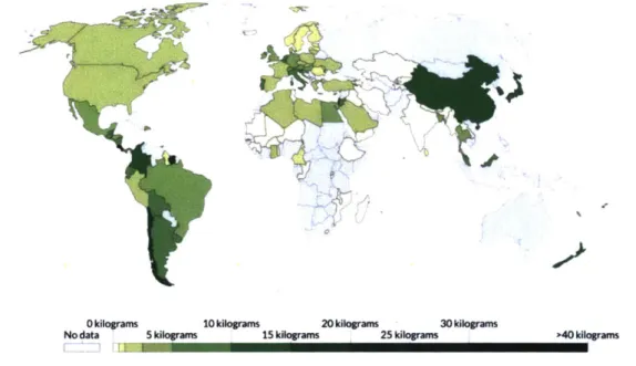
0 kilograms 10 kilograms 20 kilograms 30 kilograms

No data 5 kilograms 15 kilograms 25 kilograms >40 kilograms Source: UN Food and Agricultural Organization (FAO) CC BY

Figure 1-1: Pesticide use per hectare of cropland in 2008. Average pesticide application per unit of cropland, measured in kilograms per hectare - Taken from Roser and Ritchie 2013. [1]

According to the Indian Veterinary Research Institute,

90,000 metric tons of technical grade pesticides are used annually in India to

control pests and plant diseases. The majority of these pesticides are beneficial when used for specific purposes, handled properly and applied as per the recommendations of the manufacturer. However, over the years, there has been a mounting fear and concern that indiscriminate and in-proportionate use ofpesticides may lead to their residues in the food chain where they may exert their harmful effects on human beings and animals. In an ideal pesticide application, the chemical should fall exactly on the target and be

degraded completely to harmless compounds but this never occurs and only some part of the pesticide hits the target pests while the remainder drifts into the environment. [2]

Indeed, there is a balance to be struck in applying just the right amount of pesticides to reap their benefits without causing harm to the environment. However, there are no existing technologies that effectively aid farmers in monitoring the amount of pesticides they apply to their crops. From the perspective of the average farmer, it is better to overshoot the amount of

pesticides they are using and risk contributing harmful pollution, than undershoot the amount of chemicals they are applying and end up with a low yield. Given present day demands for food products and rigorous competition among agricultural suppliers, farmers are left with few alternatives to using these harsh chemicals in their work flow. As a result, excessive pesticide use is increasing all around the world.

1950 1960 1970

Year

1980 1990

Figure 1-2: Total global pesticide production and global Taken from Tillman et al. [3]

pesticide imports, 1940s- 2000

-As the use of pesticides continues to rise globally, we see that the harmful effects of excessive pesticide use are not limited to the environment. Pesticide residues have been found to cause immune system problems in animals as well as carcinogenic effects and reproductive disorders in both animals and humans. [1]

C U C .20 .0) 6 3.0 2.01 1.0 0.0 19 * Pesticide production * Pesticide Imports 12 110 12 0 t: R-C

.g 0

W

PeetiM residue in human onue. Unitd ate". Ip HCH (OC) kNOgrs 4 0 DDE- T 3 190 1973 19697 197 19683

Peal baaal) in huanb9 40 UadK~t 30 2.5 Deekdnn MWn4m Pe 2 0 MD HCH (BCH) 1 L -OM (9MT 10 DDE 05 0 0 19 77-6 196-7 1971 1976-77 196-83

Figure 1-3: Pestiide residue levesh in humain huadios tiseadMuaWilnUA 1120 0 Mahgrams PIK 70 kafe 1we so n PCs Mdk b") so C HCH (8NC) 30 tZ DDT COMPLEX 20 10 1976 1978 1980 1 982 1 9I4 1977 1979 1981 1983 1905

Figure 1-3: Pesticide residue levels in human adipose tissue and human milk in USA,

1970-1983, United Kingdom, 1963-1983, and Japan, 1976-1985 -Simon (1996) - Taken from the State of Humanity. [19]

As shown by the figure above, these chemicals are found in nonnegligible amounts in human tissue. Though some of the harmful effects of these chemicals on human and animal health are well understood, the extent of possible damage resulting from this chemical exposure may be greater than current data reveals.

1.1.2 Addressing the Issue of Pesticide Misuse

Significant economic, political, and social phenomena have contributed to the steady escalation of pesticide use and misuse. This complex issue will require a multitude of flexible and multifaceted approaches to solve, however three potential approaches to addressing this issue are presented below.

1. Educate people, especially farmers, on the harmful effects of excessive pesticide usage. a. Formally communicate to people the health risks associated with pesticide use to

humans, animals, and the environment.

b. Inform farmers about the harmful effects of pesticide overuse and advise them to judiciously use pesticides in terms of their quantity and frequency.

2. Regulate pesticide usage and manufacturing on a governmental level.

a. Require that appropriate documentation be provided to farmers from

manufacturers of pesticides.

b. Ban or limit use of particularly harmful chemicals 3. Develop safer pesticides or alternatives to pesticides.

a. Develop Bio-pesticides like viral, bacterial or fungal pesticides or pesticides of

botanical origin which can be used in crops to kill the insect pests without

polluting the environment. [2]

b. Develop non-chemical alternatives to pesticides.

Initiative is currently being taken in all three of these categories to address the issue of excessive pesticide usage. For the remainder of this paper, we will focus on category 3 section b and explore one mechanized design solution that aims to provide a non-chemical alternative to pesticide use.

1.2 A Mechanized Design Solution

Over the last several decades there has been significant growth in the area of high-tech farming robotics. From nursery planting to shepherding and herding, dozens of agricultural robots are currently commercially available and are utilized to mechanize agricultural processes and increase productivity. [4] Given the growing acceptance and use of farming robots in today's agricultural sector, the opportunity is presented to leverage this pre-existing trend to attack the issue of pesticide abuse. We propose a farming robot that is able to target and mechanically "zap" both invasive insects and plants with a highly pressurized jet of steam. Previous innovations at MIT in the Bioinstrumentation Lab in jet ejection technology encourage the feasibility of this type of approach.

Figure 1-4: Concept illustration depicting a farming robot that is able to navigate through agricultural fields, target harmful pests, and eliminate them with a high-pressure jet of steam.

One notable design challenge in bringing this concept to reality is in the manipulation of the jet ejector element which is mechanically targeting the pest. In order to accomplish the task of quickly tracking a moving target as small and evasive as a fly, the manipulator must be capable of traversing a large angle range at very high speeds. The remainder of this thesis focuses on the design and development of the manipulator for this desired motion in this particular use case.

Chapter 2

Top Level Design

In this chapter we review a key enabling technology which informed the chosen design path. Additionally, the design requirements are listed and the approach to achieve these requirements is outlined.

2.1

Needle-free Jet Injection Technology

Needle-free drug delivery by jet injection is achieved by ejecting a liquid drug through a narrow orifice at high pressure, thereby creating a fine high-speed fluid jet that can readily penetrate skin and tissue. Until very recently, all jet injectors utilized force- and pressure-generating principles that progress injection in an uncontrolled manner with limited ability to regulate delivery volume and injection depth. [5] In an effort spearheaded by Andrew Taberner, N. Catherine Hogan, and Ian Hunter, the Bioinstrumentation Lab at MIT has developed a new needle-free injection technology that addresses the shortcomings evident in pre-existing technologies.

The device developed by the Bioinstrumentation Lab is controlled by a custom high-stroke linear Lorentz-force motor that is feed-back controlled during the time-course of an injection. Using this device, the speed of the drug jet and the volume of the drug being delivered is able to be monitored and modulated continuously in real time during the injection process. The lab has demonstrated the ability to control injection depth (up to 16 mm) and repeatably and precisely inject volumes of up to 250 mL into transparent gels and post-mortem animal tissue. [6]

SPiston jet

Magnet

180 MM _Ampoule

Figure 2-1: (a) Handheld-injector. (b) Cutaway view of linear Lorentz-force motor. (c) cRIO controller - Taken from Taberner et al.[6]

Thus far, this needle-free jet injection device has been experimentally tested and validated with a wide range of typically injected drugs and macromolecules. We believe we will be able to repurpose this technology to eject various other types of liquids at high speeds for a multitude of applications beyond needle-free injection in medical settings.

We now highlight the potential for this technology to be applied to the area of high-tech farming robotics, more specifically to facilitate the elimination of harmful and excessive use of pesticides. In order to adapt this jet injection technology to attack the issue of pesticide control, we suggest a repurposing of the device to eject small jets of high speed, high pressure steam. These jets of steam will be utilized to kill unwanted insects by physically "zapping" them, or rather slicing them with a high-speed jet of steam. The same method can be applied to unwanted and harmful plants, particularly invasive weeds, that pose serious threats to agricultural yields. Though it is necessary to totally uproot some vigorous weeds, like bamboo for instance, many weeds will die after just cutting off the top, as long as they do not receive water.

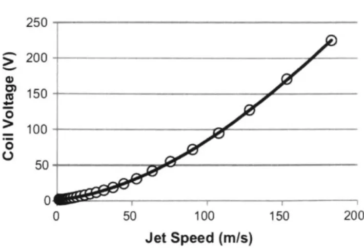
250 > 200 0S150 100 0 50-0 50 100 150 200 Jet Speed (m/s)

Figure 2-2: Typical feed-forward model relationship. Measured points (open circles) and polynomial fit (line). This data corresponds to a liquid injection material - Taken from Tabemer

et al. [6]

As shown in Figure 2-2, the jet injector is able to achieve liquid jet speeds over 150 m/s.

Considering that a steam jet is much less massive than a liquid jet, it is reasonable to assume that we will be able to achieve equal, if not higher, speeds after adapting this technology to eject steam. For example, an impulse of 0.01 seconds with 1mg of steam would generate a 15 N force

on the bug. This should be more enough to kill the bug, without just washing it away. One standing issue is to control the ejection so the plant the bug is on does not get sliced and harmed in the process.

2.2

Targeted Pesticides

Although there are many forms of pesticides that target rodents, fungi, bacteria in

addition to insects and other plants, we intend to target only invasive insects and plants with our technology. Below we show a larger scope breakdown of pesticides used, and see that

Other pesticides 250,000 tons 200,000 tons 150.000 tons 100.000 tons 50,000 tons 0 tons 1990 1992 1994 1996 1998 2000 2002 2004 20

Source UN Food and Agricultural Organization (FAO)

Figure 2-3: Pesticide breakdown by type, United States. Broken down by product type, measured in tons of active ingredient - Taken from Roser and Ritchie. [1]

By limiting our scope in targeting only insects and plants we will still be able to address a significant portion of the pesticide problem. The jet injection technology previously developed by the lab provides an opportunity to innovate an alternative to pesticide use that eliminates the need for chemicals entirely. The design of the parallel manipulator discussed in the rest of this paper takes this jet injector technology as a central component to mechanical design decisions.

2.3

Existing Parallel Spherical Rotation Mechanisms

A commonly used parallel manipulator is the Gough-Stewart platform which contains six prismatic actuators, commonly hydraulic jacks or electric linear actuators, attached in pairs to three positions on the platform's baseplate, crossing over to three mounting points on a top plate. All 12 connections are made via universal joints. Devices placed on the top plate can be moved in the six degrees of freedom in which it is possible for a freely-suspended body to move. These are the three linear movements x, y, z (lateral, longitudinal, and vertical), and the three rotations (pitch, roll, and yaw). [8]

lop or mobile plate

Ip per legs

yindrical joints

Lmwer legs

wer universal joints

Fied base plate

Figure 2-4: Gough-Stewart platform six degree of freedom parallel manipulator - Taken from Kerr. [8]

This design for parallel manipulation is very well suited for applications in flight simulators, mechanical testing, and other situations that require fast and precise manipulation of small angle ranges. However, this design is not ideal for large angle ranges because a very large height discrepancy is required in order to change the angle. As show in the figure below, a large angle change would require analogously large motion from the prismatic actuators.

Figure 2-5: Stewart platform geometry is not ideal for large angle changes as they require very large changes in actuator length to achieve. Inertial effects make this motion difficult to perform

quickly.

I

As a result, this geometry is not ideal for large angle parallel manipulation and a new geometry needed to be ideated to meet our design requirements.

2.4

Design Requirements

This section focuses on the mechanical design for the parallel manipulator of the jet ejector.

Requirement 1: The mechanism must achieve at least one full hemisphere of spherical rotation. Design Decision: Actuators are able to manipulate through a range of 180 degrees of spherical motion. Five bar linkage with 3D arrangement allows us to achieve this motion.

Requirement 2: The mechanism must be able to travel at speeds matching the fastest invasive insects (fastest flying insect is a dragonfly which can traverse between 13.4 to 26.8 m/s).

Design Decision: Actuators will be configured in parallel so that the second actuator does not need to account for inertial effects of the first.

Requirement 3: Require precise position control of the mechanism.

Design Decision: Utilize servo motors to achieve precise control. Two points of actuation control three degrees of freedom.

Requirement 4: Mechanism linkages must be as light as possible to minimize inertial effects hindering high speeds.

Design Decision: Manufacture linkages with high strength carbon fiber composite. Minimize heavy metal elements such as bearings.

Requirement 5: Design must avoid mechanical interferences.

By meeting these five design requirements we are able to design a prototype for this type of parallel manipulator in our specified use case.

2.5

Design Concept

The design of the parallel spherical rotation mechanism was inspired by a similar parallel drive mechanism invented by Professor Ian Hunter shown below.

If

b

Figure 2-6: Parallel spherical manipulator with four actuator and six degrees of freedom developed by Professor Ian Hunter in 1990.

This design, while not meeting requirement 4, does realize our remaining design objectives. The rest of this thesis focuses on the simplification, miniaturization, and adaptation of this design to fit the requirements of our specific use case.

Chapter 3

Design & Device Fabrication

In this chapter we review the design of the parallel spherical rotation mechanism, the iterations that the design went through, the fabrication of the mechanism, and the kinematic modeling of the mechanism.

3.1

Design Exploration

Before committing to a particular design, significant time and effort was spent creating low level prototypes in order to gain an intuitive understanding of how the system behaved and moved through 3D space. Below we see a preliminary prototype of a five-bar linkage mechanism with linkages of quarter circle geometry. The links all share a common center point but have different radii in order to avoid interferences when rotated.

/2

4 )

A

Figure 3-1: A: Five-bar linkage with quarter circle linkages. The yellow linkages have the same radii. The grey and orange linkages are of decreasing radii. Handles allow for easy rotation by

hand. B: Shows nesting of linkages when rotated.

All solid modeling was done in the CAD software system Onshape. [15] Before discussing the benefits as well as the shortcomings of this design, we will set a coordinate system and a convention for referring to the different linkages present.

n4.1 Fr iii

n3.

Figure 3-2: L I radii =100 mm, L4 radii =100 mm, L3 radii =80 mm, L2 radii =60 mm. W-77777W

p

- -- I

As shown in the figure above, each link, as well as its nodes are labeled. Ultimately, the goal of this mechanism is to control the motion of node n3.2 which is constrained by the other linkages to move on the surface of a sphere depicted in the coordinate system shown below.

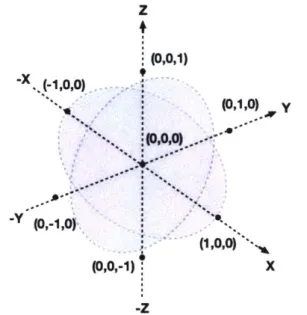
z (0,0,1) (-1,,0) (0,1,0) y -y (0,-1,00 (1,,O~ (0,0,-1) x -z

Figure 3-3: The gray circle represents the surface of motion of node n3.2. We use a unit coordinate system with the point (0,0,0) located at the center to simplify the mathematics referring to the position of n3.2. This normalized coordinate system also helped simplify the

math when figuring out the kinematics in section 3.2.

The equation of a sphere representing the grey area in the figure above is,

(x -

+ (y -

where (a, b, c) denotes the center of the sphere. In this coordinate system, we see that actuator one which controls our input angle P1 is located at (-1, 0, 0). Similarly, actuator two which controls our second input angle 42 is located at (0, 1, 0). To give some basic intuition for the

system, we can think of it as a two-step process. First, we rotate linkage Li to set q51. This rotation sets a new axis of rotation along the axis of the revolute joint at node n2.1. Second,

we rotate L4 to set /2. As this rotation is carried out, node n3.2 rotates about the new axis

set by the first rotation. The figure below gives a visual description of this motion.

'P

2

~mm~

Figure 3-4: The first input rotation sets our new axis of rotation. The second input rotation controls the rotation of node n3.2 around the new axis of rotation. The angle n3.2 which

traverses around this new axis of rotation is exactly equal to

/2-Returning to our first low level prototype, below is an image of the fabricated device.

Figure 3-5: The parts for this prototype were 3D printed and laser cut for fast turnaround time. A .;A

Though the linkages were designed to nest within each other, this design still caused

interferences that made continuous transfer between the upper and lower hemisphere of rotation very difficult.

Figure 3-6: Interferences occur at q1 = 900, 0 2 = 900 as well as

#

prevents quick and continuous transfer of node n3.2 from the lower hemisphere to the upper hemisphere.

In order to address these issues, the second low level prototype ellipse shaped linkages were made. This avoided interferences in both rotation axes.

Figure 3-7: Prototype number two with elliptical shaped linkages. Additionally, two 3D printed parts were added connecting laser cut pieces to the center to add more rigidity to the frame

Though this design eliminated mechanical interferences, it resulted in n3.2 being directed to move on the surface of an ellipsoid rather than a sphere. Although eliminating possibilities for interferences would reduce risk of the mechanism breaking, this geometry would make the mathematics more difficult when determining the kinematics for the mechanism. This trade off was considered and ultimately, I decided to first figure out the kinematics for the simpler spherical rotation before tackling more complicated geometries. The following equation,

x 2 _y 2

z 2

-+ + - = 1, ₍₂₎

a2 b2 ce ₍₂₎

represents an ellipsoid where (a, b, c) denotes the center of the ellipsoid.

Figure 3-8: The parts for this prototype were 3D printed and laser cut for fast turnaround time. As shown by these prototypes, depending on the shapes of the linkages, the mechanism could be

3.2

Device Modeling

3.2.1 Degrees of Freedom

Linkages with multiple degrees of freedom need more than one driver to precisely operate them. Generally, mutli-degree of freedom mechanisms are open loop kinematic chains that are actuated in series and used for reaching and positioning, such as robotic arms. Our proposed device is a closed loop kinematic chain actuated in parallel to control three degrees of

freedom. Although there are only two points of actuation, we expect to require three kinematic equations to fully describe the position of the mechanism at any point in time. Because of this

inconsistency with most multi-degree of freedom mechanisms, traditional methods to solve for the kinematics of the system did not generate useful results.

For example, Gruebler's equation was used to confirm the number of degrees of freedom of the system. When using this equation, different types of joints result in different f values. Higher pair joints are classified as those with surface contact such as revolute and prismatic joints, receiving a value of f= 1. Lower pair joints are classified as those with point, line, and curve contact such as pin in slot joints. These lower pair joints receive a value of f= 2. Certain joints can even count as f= 0.5, 1, 2, or 3. [9] Gruebler's Equation,

F = 3(n - 1) - 2f, = 3(5 - 1) - 2 * 5 = 2 DOF, (3)

Is used to discern the number of degrees of freedom of the mechanism where n= total number of links, f_1 = total # of joints. Gruebler's equation does not account for link geometry and

therefore can lead to misleading results, especially in 3D mechanisms. [9] Though the equation tells us there are two degrees of freedom, and this initially makes sense considering that there are two actuators controlling the motion, there are actually three pieces of information essential to fully determining the position of the mechanism. The first kinematic equation includes

information about the first actuator while the second kinematic equation contains information about the second actuator. When these two equations are solved, we get two solutions. The third

piece of information required for uniquely determining the location of node n3.2 is which hemisphere you are operating in.

3.2.2 Identifying Singularities

At a singular configuration, at least one direction in which the robot cannot generate

non-zero velocity at the end-effector. At the points q1 = 900, 52 = -90* as well as

#1l

#2

'Pl

Figure 3-9: Solid model of prototype configured at position points 51 = 90*, P2 = -90*. The dotted line shows the infinity of solutions for n3.2 in this configuration.

In order to deal with this singularity in the mechanism, we decided to simply avoid crossing this configuration. Though the mechanism has the ability to traverse a full 360 degrees of spherical rotation, for our application in farming robotics, only a full 180 degrees of spherical rotation is required.

3.2.3 Trying to Solve Kinematics Intuitively

Initially I tried to compute the kinematic equations of the mechanism by applying the same intuition presented in Figure 3-4. By this logic, the final position of node n3.2 can be calculated in two steps. First,

#1

the angle of rotation node n3.2 traverses around this new axis, fl where fl is exactly equal to

42-Simple geometry was used to calculate the new axis of rotation from our first input angle

#1a.

cos 02 + (R cos (p)2 (1 - cos 02) R2 _{cos (1 sin 4P1 (1 - cos 02) R sin (p, sin 02}

R = R2 cos 01 sin (1 (1 - cos 02) cos 02 + (R sin (1p)2(1 - cos 02) -R cos 01 sin 02 (4). -R sin 01 sin 02 R cos (1 sin 02 COs 02

We are then able to calculate the new position of node 3.2 by the following equation,

n3.2 xn₃.₂ = n3.2 R Yn3.2 . (5) Z fn3.2. Zn3.2

One problem with this method of computing our forwards kinematics is that it is not able to be back solved analytically. Additionally, it requires information about the previous position of node n3.2 in order to calculate the next position. We found a simpler way to solve the kinematics

of the system was by leveraging the symbolic computation software, Mathematica [16].

3.2.4 Implementing in Mathematica

Any pair of input angles (01, 02) correspond to some (x,y) position on the surface of a sphere. Since we know the geometry of the linkages confines node n3.2 to move on the surface of a sphere, we can apply this constraint to solve for the pair of z values that correspond to the calculated (x,y) position. Since we are only concerned with the top hemisphere of rotation, we take the positive z value solution as our answer. To simplify the model, we treat all linkages

as the same radius of unit value. In cohesion with the coordinate system presented in Figure 3-3 positive rotation of both qfj and 0 2 are determined by the right-hand rule where a rotation

pointed towards the center point at (0,0,0) is considered positive.

L1I n2.1 1.2 z (0,0,1) (0,1,0) y .Y. -y(09-190iJ (1,0,0) (0,0,-1) X -z

Below we show how the constraints of our problem were applied in Mathematica.

1. Set positions of actuator 1 and actuator 2 at positions (-1, 0, 0) and (0, 1, 0) respectively. 2. Constrain nl.2 to move in circle in YZ plane.

3. Constrain n4.2 to move in circle in XZ plane.

4. Apply the length constraint between nodes n 1.2 and n3.2 by subtracting the location of

ni.2 from the location of n3.2 being calculated.

5. Apply the length constraint between nodes n4.2 and n3.2 by subtracting the location of n4.2 from the location of n3.2 being calculated.

6. Apply constraint of motion of node n3.2 on the surface of a sphere of unit radius. 7. Solve for final position of node n3.2 in cartesian coordinates (x, y, z) given an arbitrary

(01, 0 2) input.

8. (Optional) Convert cartesian coordinates into polar coordinates.

In order to solve the mathematical inversion problem, we follow steps 1-6 as they are presented

above but alter steps 7 to the following.

7. Solve for final position of actuators one and two (p1,

#

Forwards Kinematics

Inputs: input angles (01, 0 2)

Outputs: position of n3.2 in cartesian coordinates (x, y, z) Top hemisphere equations

Equations deriving (x, y, z) position of node n3.2 from the input of (41, 42) in the

upper hemisphere of rotation,

- -((sec412Vcos (p12 COS 02 ₂2(3+cos 24)2)+2 cos 2(p, sin 422tan 42)

(6)

(2+2 COS 02 2tan q)12)

-((sec 4)22Icos 12 cos $ 2

2

(3+cos 2(2)+2 cos 24) sin 422 tan $1)

(2+2 cos (p12 tan 422)

Cos 4)12 cos 022(3+cos 24)2)+2 cos 2$p1 sin 022

2 (cos 2$) +cos 2 sin (p₁2)

(7)

(8)

Bottom Hemisphere Equations

Equations deriving (x, y, z) position of node n3.2 from the input of (01, 4)2) in the

lower hemisphere of rotation,

= -((sec 412Vcos4$₁2 cos $ 2

2_{(3+cos 242)+2 cOS 24)1 sin (22 tan 42)} (2+2COS 02 2tanqb,2)

-((sec$P 22Vcos$012 cos$02 2

(3+cos 2$2)+2 cos 2(p, sin) 2 2 tan 01) (2+2 cos 4)12tan$22) (9) (10) (11)

cos 12 cos 0222(3+cos 2(P2)+2 cos 2qbl sin 022

2(cos 2$)2+cos 02 2sin $p12)

Once the (x, y, z) position of n3.2 is determined from the two input angles, we may convert to polar coordinates by use of the following equations,

x = rsinacosO,y = rsinasint9,z = rcosa, (12)

r = x2 + y2 + z 2, (13) a= cos- 1, (14) y sin sin- * r . (15)

z

0Cr

We are able to convert from the Cartesian coordinates derived from the forwards kinematics equations, to polar coordinates. Since we want to control the position of node n3.2 is 3D space, the end goal is to have a system where the desired vector position of node n3.2 can be specified and then the necessary (f1,

#

3.2.6

Mathematical Inversion

Inputs: position of n3.2 in cartesian coordinates (x, y, z)

Outputs: input angles (41, 0₂)

Top hemisphere equations

Equations deriving the (#1, 42) position of our actuators from the input of a desired (x, y, z) location in the upper hemisphere of rotation,

-1 (-4x2y)+(4ylx 2J)4(y2(4X2 -4lx2 = cos 02 = cos~' 12) -4(-4+4x2)(4_4X2 _x4_-4y2+2x2X2 Ix 41) 8(-1+x2 ) (4y2 X)-(4xy2 )- (x2(-4y2

+41y2|I2)-4(-4+4y2)(4_4x2 -y4-4y 2+2y2 y2

_ y4I) 8(-+y2

)

(16)

(17)

Bottom hemisphere equations

Equations deriving the (qb1,

#

location in the lower hemisphere of rotation,

-Cos-I(-4x2y)+(4ylx2I) _ (2(42_42) 2)-4(-4+4x2)(4_4X2 -x4-4y 2+2x 2 JX2 I_X41)

1 = -cs -1( 2 y)(

_)-8(-1+x

3.3 Component Selection

3.3.1 Motor Specifications

Now that we have the equations necessary to control the mechanism. We need to choose an actuator that will meet our needs in terms of speed, precision, and angle range.

VS-1I Servo NEMA 11-size XD-3420 Brush DC Stepper

Stall Torque (N.m) 1.47 .059 0.19 (24v)

No Load Speed (deg/s) 272.7 15,000 36,000 (24v)

Output Angle (deg) >= 170 360 continuous 360 continuous

rotation 1.80 step rotation

angle

(200 steps/revolution)

Weight (g) 100 110 448

Table 3-1: Comparison of different motor specifications. [11, 12, 13]

DC motors allow for very fast and continuous rotation and are usually ideal for anything that needs to spin at high RPMs. Though we have an interest in speed, we do not require continuous rotation for this application. Additionally, DC motors are difficult to control precisely in

comparison to servo and stepper motors which makes them unideal for our use case. Though servo motors are not typically as fast as DC motors, they are well suited for robotics because of their high precision, though this precision is only within a limited angle range. Stepper motors allow for slow accurate rotation and are very easy to set up and control. They have an advantage over servo motors in positional accuracy, however in our use case precision is prioritized over accuracy. Ultimately, we decided to use the servo motor because it could handle high torques and would be able to repeatably drive to specified locations with precision. One downside of this motor is that it only has 170 degrees of range, but since we only are aiming to control the mechanism in one hemisphere, this is appropriate for our use case.

3.3.2 Material Selection

In order to reduce unwanted inertial effects that reduce speed capabilities, wewanted the linkages to be as light as possible while retaining adequate strength to hold the mass of the miniaturized steam jet ejector which I estimated at 50g. I decided to 3D print the linkages with a carbon fiber composite material on a Markforged Mark Two 3D printer. This printer allows for parts to be routed with continuous strands of carbon fiber, allowing deliberate reinforcement of the part in desired axes.

0 UL 600 500 400 300 200 100 0 0 0.01 0.02 Flexural Strain 0.03 0.04

Figure 3-12: Data provided by Markforged of the flexural stress vs flexural strain relationship of composite beams with various continuous fiber infill reinforcements. [14]

Reinforcement with continuous carbon fiber along the bending axis gives us a flexural strength comparable to aluminum at a fraction of the weight. Therefore, I decided to use this reinforce all four quarter circle linkages.

Carbon Fiber ---HSHT Al 6061-T6 Fiberglass Kevlar* Fiberglass Onyx

Figure 3-13: Fiber inlay of linkage LI displayed in Markforged slicing software, Eiger. [18]

Adding continuous fiber inlay does significantly increase the weight of the linkage. In the future, this parameter can be optimized to allow for maximum strength benefits without adding

3.4 Alpha Prototype

A solid model of the final alpha prototye utilizing the VS- 1 servo motors and composite reinforced 3D printed linkages. The frame was constructed with aluminum t-slot extrusion pieces to add weight to the system so it would not move around as the mechanism rotated. A laser pointer was attached at the central node to visually track the vector location of node n3.2 throughout testing. Acrylic laser cut pieces were used to mount the motors to the frame.

VS-11 servo

motor AA batteries

red laiser for visual

Opcking

Figure 3-15: Image of final fabricated alpha prototype. Four AA batteries provide power to the servo motors. The motors are controlled by an Arduino Teensy microcontroller.

A video of the device being manipulated to various specified locations can be found at the

Chapter 4

Device Performance

In this chapter we review some low-level testing of mechanism. We validate the mathematical inversion problem results with the forwards kinematic results as well as the true mechanism location in 3D space.

4.1

Validation of Mathematical Inversion

To check the mathematical inversion problem, I specified 25 different (41,

#

then used the forwards kinematic equations to calculate the resulting (x, y, z) position of node n3.2. I then plugged these resulting (x, y, z) positions back into the mathematical inversion equations to validate that they would calculate the same (/1, 02) pairs. The results are presented

Mathematical Inversion

Input Input X rcalcuated Y rcalculated Z cakculated

0 0 0 -0.996 0.087 0 0 85 0 0 -0.707 0.707 85 -3.4151E-06 45 0 -0.707 0 0.707 45 0 0 45 0.00 0.707 0.707 8.5377E-07 45 -45 0 0.707 0 0.707 -45 0 0 -45 -0.577 -0.577 0.577 8.5377E-07 -45 45 45 -0.608 -0.608 0.510 45 45 50 50 -0.341 -0.082 0.937 50 50 5 20 -0.904 0.074 0.421 5 20 -10 65 -0.179 -0.852 0.492 -10 65 60 20 -0.594 -0.462 0.659 60 20 35 42 -0.171 -0.171 0.970 35 42 10 10 -0.187 -0.187 0.964 10 10 11 11 -0.069 0.964 0.258 11 11 -75 15 -0.985 0.0152 0.174 -75 15 -5 80 -0.985 0 0.174 -5 80 0 80 -0.336 -0'.605 0.721 0 80 40 25 0.227 -0.843 0.487 40 25 60 -25 -0.995 -0.050 0.087 60 -25 30 85 0.577 0.577 0.577 30 85 -45 -45 -0.832 -0.277 0.480 -45 -45 30 60 -0.277 -0.832 0.480 30 60 60 30 -0.832 0.277 0.480 60 30 -30 60 0.832 -0.277 0.480 -30 60 30 -60 0 -0.996 0.087 30 -60

Table 4-1: 25 points validating the mathematical inversion equations by use of the forwards kinematic results.

This table shows spot on agreement between the forwards and backwards solved equations. We approximated the returned (#1, 02) values to the nearest whole degree, rounding calculated results such as 8.53 77 x 10-7 down to 0.

In order to visualize the location of these (x, y, z) points on the surface of a sphere, I plotted them in MATLAB. This model allowed me to visually check the output of the alpha prototype to the true calculated (x, y, z) value. Just by observation it was clear that there was very good agreement between the calculated values and the position met by the prototype. In the future a more robust 3D optical tracking system could be implemented to better validate the accuracy and precision of the prototypes motion.

Forwards Kinematics

100 50 N 0 -50, -100 100 Laser Location s0 0 50 0 -50 -50 x -10 V10 -100 60 -100 -40 -W -40 -20 0 20 40 00 80 100 Y 100

Figure 4-1: 25 points from Table 4-1 plotted on the surface of a sphere for visual aid in validating device performance.

Once the basic performance of the prototype was validated, I wrote a MATLAB script to take in the desired position of node n3.2 in polar coordinates, convert this position to cartesian

coordinates, and back solve for the necessary (01, 02) pair using the mathematical inversion equations. [17] The script then interfaces with the Arduino Teensy to drive the motors to the desired angles.

4.2

Precision Testing

It is important that the device is repeatable and does not experience drift in position over time. To validate this, I set up a test that cycled the device through three positions, pausing for three seconds at each specified position. During the first cycle of the experiment I marked the position of the laser at each of the three positions. I ran this experiment for twenty-five minutes and then re-measured the position of the laser at all three positions. At (01 = 0, P2 = 0), the

laser position experienced no significant drift. At positions (01 = 0, P2 = 45) and (4g. = -45,

02 = 0) 1 was able to measure a positional difference of less than one millimeter. This most

likely was not the result of motor drift but rather an amplification of laser misalignment which is more visually apparent at shallow angles that cause the laser to traverse a greater distance.

F

o ~, ~

4~ 0

0W

Figure 4-2: Still image of the set up during the twenty-five-minute-long precision test.

A video of a portion of the precision test can be found at the following link: https://www.dropbox.com/s/904oe9fynj7w7i0/IMG_1 877.mov?dl=O

4.3

Speed Testing

The speed of the device was measured from the video data collected during the precision test. Five points were collected to attain a statistically significant measurement of the speed of the device.

Distance Imm] Time is] Speed Im/si

Trial 1 122.57 0.32 0.38 Trial 2 122.57 0.34 0.36 Trial 3 122.57 0.34 0.36 Trial 4 122.57 0.35 0.35 Trial 5 122.57 0.32 0.38 Average Speed - - 0.366 + 0.012

Table 4-2: Data collected from speed test to discern average speed.

Unfortunately, due to limitations of the speed of our servo motor, this average speed does not meet our design requirements. However, due to the parallel design of the mechanism, it has the capability to achieve much higher speeds by simply replacing the servo motors.

Chapter

5

Next Steps

5.1

Improvements

This preliminary work on designing and controlling this parallel spherical rotation mechanism has given several insights on how a system like this can be improved upon in the future. The alpha prototype has validated the geometric design of this device to achieve our desired spherical motion. Additionally, the kinematic equations and mathematical inversion equations provide a framework for controlling the device through 3D space. The prototype meets our design requirements in terms of precision and angle range, but falls short on the metric of speed. Although the servo motors currently included in the design are not able to perform at very high speed, we expect this to be fairly simple to improve in the future as the speed is currently limited only by the capabilities of the motors, not the capabilities of the mechanism itself.

We can improve our precision measurements by creating a 2D grid with IR sensors and randomly generating a desired target point and then driving the laser to that point. By using the

IR sensors to collect position data we will be able to calculated a more quantitative precision measurement. The device itself can also be further improved by reducing weight in the linkages and by reducing friction in the bearings that inhibit quick motion.

5.2

Future Research Directions

In the future it would be very beneficial to build a state space model for the mechanism so that the position as well as the velocity and the path traveled by the mechanism can be controlled. This path dependent model would improve the ability to control the system since we would no longer need to avoid singularities like the ones discussed in section 3.2.2. This would enable us to freely control the device through the entire 360 degrees of rotation it is capable of achieving.

It would also be beneficial to build a new and more robust prototype of the device that will be able to undergo more rigorous validation and testing and would be able to interface with the state space model.

Bibliography

[1] _{Roser, M, and Ritchie, H. "Fertilizer and Pesticides." Our World in Data, 26 Oct. 2013,} ourworldindata.org/fertilizer-and-pesticides.

[2] Chauhan, R.S. & Singhal, L. (2006). Harmful effects of pesticides and their control through cowpathy. Int. J. Cow Sci.. 2. 61-70.

[3] _{Tilman, D. and Cassman, K.G. and Matson, P.A. and Naylor, R. and Polasky, S., Nature} (2002) 418.6898, 671-677. Date added 2019-05-09. doi: 10.1038/nature 1014. URL: https://doi.org/ 10.103 8/nature0 1014

[4] _{UK-RAS Network. Agricultural Robotics: The Future of Robotic Agriculture . 2018,} arxiv.org/pdf/1 806.06762.pdf.

[5] R. M. J. Williams, N. C. Hogan, P. M. F. Nielsen, I. W. Hunter and A. J. Tabemer, "A computational model of a controllable needle-free jet injector," 2012 Annual

International Conference of the IEEE Engineering in Medicine and Biology Society, San

URL: http://ieeexplore.ieee.org/stamp/stamp.jsp?tp=&arnumber-6346362&isnumber-63

45844

[6] _{Tabemer A, et al. Needle-free jet injection using real-time controlled linear Lorentz-force} actuators. Med Eng Phys (2012), doi: 10.10.16. j.medengphy.2011.12.010

[7] _{Hogan, N.C. and Taberner, A.J. and Jones, L.A. and Hunter, I.W, "Needlefree delivery}

of macromolecules through the skin using controllable jet injectors," 2015. Expert

Opinion on Drug Delivery. doi:10.1517/17425247.2015.1049531. URL: https://doi.org/10.1517/17425247.2015.1049531

[8] _{Kerr DR. Analysis, Properties, and Design of a Stewart-Platform Transducer. ASME. J.}

Mech., Trans., andAutomation. 1989, 25-28. doi:10. 1115/1.3258965.

[9] _{"Gruebler's Equation ~ ME Mechanical." ME Mechanical, 10 June 2017,} memechanicalengineering.com/grueblers-equation/.

[10] _{Jia, Y. Transformations in Homogeneous Coordinates. 23 Aug. 2018,} web.cs.iastate.edu/~cs577/handouts/homogeneous-transform.pdf.

[11] _{Vigor Precision LTD. VS-11 Servo.}

vigorprecision.com.hk/uploadfile/20120530/20120530150204367.pdf.

[12] _{CHANGZHOU SONGYANG MACHINERY & ELECTRONICS NEW TECHNIC} INSTITUTE. Hugh Torque Hybrid Stepper Motor Specifications. 2012,

www.pololu.com/file/0J686/SY28STH32-0674A.pdf.

[13] Permanent Magnet DC Motors. moog.com/1iterature/MCG/moc23series.pdf.

[14] _{Markforged. Material Datasheet Composites. 15 Apr. 2019,} static.markforged.com/downloads/composites-data-sheet.pdf.

[15] _{"Onshape Product Design Platform." Onshape Product Design Platform,} www.onshape.com/.

[16] _{"Wolfram Mathematica." Wolfram Mathematica: Modern Technical Computing,} www.wolfram.com/mathematica/.

[17] "MATLAB." Math Works, www.mathworks.com/products/matlab.html.

[18] _{"Eiger Software | Markforged." Markforged Industrial Strength 3D Printing,} markforged.com/eiger/.