HAL Id: hal-00317412
https://hal.archives-ouvertes.fr/hal-00317412
Submitted on 14 Jun 2004
HAL is a multi-disciplinary open access
archive for the deposit and dissemination of
sci-entific research documents, whether they are
pub-lished or not. The documents may come from
teaching and research institutions in France or
abroad, or from public or private research centers.
L’archive ouverte pluridisciplinaire HAL, est
destinée au dépôt et à la diffusion de documents
scientifiques de niveau recherche, publiés ou non,
émanant des établissements d’enseignement et de
recherche français ou étrangers, des laboratoires
publics ou privés.
times: their characteristics and predictability
P. Ritter, H. Lühr, S. Maus, A. Viljanen
To cite this version:
P. Ritter, H. Lühr, S. Maus, A. Viljanen. High-latitude ionospheric currents during very quiet times:
their characteristics and predictability. Annales Geophysicae, European Geosciences Union, 2004, 22
(6), pp.2001-2014. �hal-00317412�
SRef-ID: 1432-0576/ag/2004-22-2001 © European Geosciences Union 2004
Annales
Geophysicae
High-latitude ionospheric currents during very quiet times: their
characteristics and predictability
P. Ritter1, H. L ¨uhr1, S. Maus1, and A. Viljanen2
1GeoForschungsZentrum Potsdam, Telegrafenberg, D-14473 Potsdam, Germany
2Finnish Meteorological Institute, Geophys. Res. Div., P.O. Box 503, FIN-00101 Helsinki, Finland
Received: 24 July 2003 – Revised: 4 December 2003 – Accepted: 14 January 2004 – Published: 14 June 2004
Abstract. CHAMP passes the geographic poles at a distance
of 2.7◦ in latitude, thus providing a large number of mag-netic readings of the dynamic auroral regions. The data of these numerous overflights were used for a detailed statisti-cal study on the level of activity. A large number of tracks with very low rms of the residuals between the scalar field measurements and a high degree field model were singled out over both the northern and southern polar regions, inde-pendently. Low rms values indicate best model fits and are therefore regarded as a measure of low activity, although we are aware that this indicator also has its limitations. The oc-currence of quiet periods is strongly controlled by the solar zenith angle at the geomagnetic poles, indicating the impor-tance of the ionospheric conductivity. During the dark polar season, about 30% of the passes can be qualified as quiet. The commonly used magnetic activity indices turn out not to be a reliable measure for the activity state in the polar region. Least suitable is the Dst index, followed by the Kp. Slightly
better results are obtained with the P C and the IMAGE-AE indices. The latter is rather effective within a time sector of
±4 hours of magnetic local time around the IMAGE array. The orientation of the interplanetary magnetic field (IMF) is an important controlling factor for the activity. This is also supported by the prevailing FAC distribution during quiet times, which resembles the typical NBZ (northward Bz)
pat-tern. In a superposed epoch analysis we show that the merg-ing electric field is a suitable geoeffective solar wind parame-ter. Based on the size of this electric field and the solar zenith angle at the geomagnetic poles, a prediction method for quiet auroral region periods is proposed. This may, among others, be useful for the data selection in main field modelling ap-proaches.
Key words. Ionosphere (auroral ionosphere; electric fields
and currents; ionosphere-magnetosphere interactions) –
Magnetospheric physics (solar wind-magnetosphere interac-tions)
Correspondence to: P. Ritter
(pritter@gfz-potsdam.de)
1 Introduction
The magnetic activity at high latitudes is influenced by a number of different current systems. These are driven pri-marily by field-aligned currents (FACs) caused by plasma convection or pressure gradients in the outer magnetosphere. At times when the magnetosphere is very quiet the FACs calm down. During those times it may be possible to ob-serve the response of the auroral ionosphere to electric fields produced internally by thermospheric wind dynamo actions (Campbell, 1997).
The determination of the internal magnetic field at high latitudes is notoriously difficult, because of the large mag-netic variations which are commonly encountered in these regions. Field modelers are therefore very much dependent on reliable criteria for a quiet time data selection.
The degree of ionospheric activity is primarily controlled by the solar wind-magnetosphere interaction. The influence of the solar wind increases when the interplanetary magnetic field (IMF) develops a southward component (negative Bz).
The dependence of the magnetic activity on the orientation of the IMF has been investigated in many studies (e.g. Hir-shberg and Colburn, 1969; Akasofu, 1979; Weimer, 1995). During northward IMF the activity is much reduced, but the solar wind-magnetosphere interaction is still poorly under-stood for this configuration (Vennerstrøm et al., 2002). In a recent study, Stauning (2002) showed, that for large positive
Bzabove 5 nT, the FACs become stronger again.
The other factor influencing the current intensity is the ionospheric conductivity. Primarily, the source for the gener-ation of charged particles in the ionospheric E-region is the solar extreme ultra-violet (EUV) radiation. In the auroral re-gion, another aspect is quiet effective: collisional ionisation caused by precipitating, energetic electrons which are associ-ated with intense FACs (Baumjohann and Treumann, 1996). Hence we can expect reduced activity at night, in particu-lar during the dark poparticu-lar winter outside magnetic storm and substorm periods.
0 5 10 15 20 rms [nT] North Pole: RMS 0 10 20 30 40 50 occurrence rate in %
Sep00 Dec00 Mar01 Jun01 Sep01 Dec01 Mar02 Jun0220
40 60 80 100 120 χ [°]
distribution of quiet orbits
0 5 10 15 20 rms [nT] South Pole: RMS 0 10 20 30 40 50 occurrence rate in %
Sep00 Dec00 Mar01 Jun01 Sep01 Dec01 Mar02 Jun0220
40 60 80 100 120 χ [°]
distribution of quiet orbits
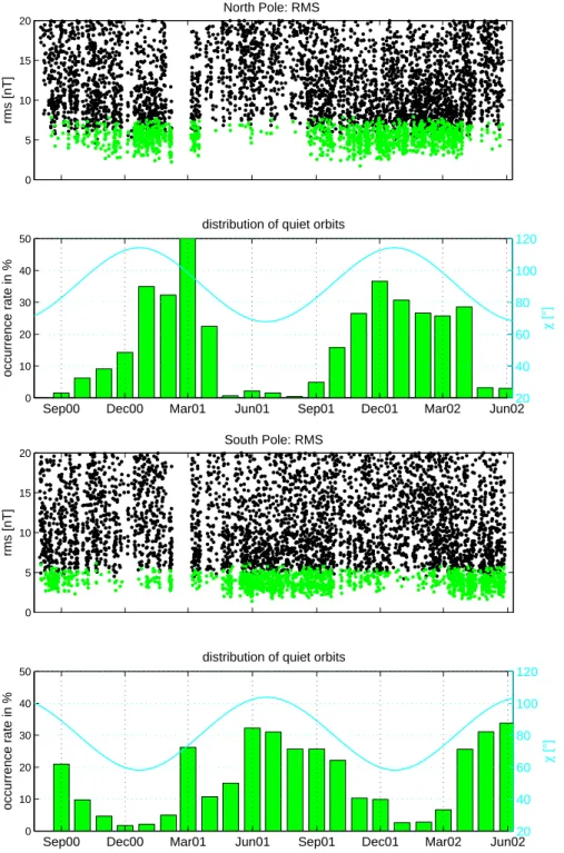
Fig. 1. Top panel: Disturbance level of the polar regions versus time. The green dots mark the low values assigned for the very quiet passes. Lower panel: occurrence of quiet passes and variation of solar zenith angle at the geomagnetic poles (θ, φ=81.8◦, −82.5◦and −74.3◦,125.5◦). At zenith angles of less than 80◦almost no quiet events are encountered (the results of March 2001 are biased due to a large data gap).
It has been reported repeatedly that the indices used com-monly for magnetic activity, like Kpor Dst, are not suitable
for characterizing the activity in the polar regions (e.g. Xu, 1989). In the literature, quite different criteria can be found which are used by various groups for selecting high lati-tude quiet periods. Sillanp¨a¨a et al. (2004) used the condi-tion Kp≤1.3 at a time 3 h before the event for their study of
quiet days, and additionally, the auroral activity index for the IMAGE array (IMAGE-AE, cf. Kauristie et al., 1996) had to be less than 100 nT. For the purpose of main field mod-elling Olsen (2002) selected the data according to the follow-ing conditions: Kp≤1.3 at the time of the observation, Kp
≤2.0 for the preceding 3 h, |Dst|<10 nT, |d(Dst)/dt |<3 nT
A rather different approach was applied by Maus et al. (2002). For their study of modelling the lithospheric magnetisation from CHAMP observations they inspected all polar passes regardless of the prevailing magnetic activity. Their criterion was the root-mean-square (rms) value of the variations in the residuals between a high degree field model and the scalar field magnitude detected in the auroral regions. Passes with an rms value below a certain threshold were clas-sified as being quiet.
In the study presented here, we make use of this collection of quiet orbits. By doing so, we take the opposite path to many other researchers who used solar wind parameters for classifying their ionospheric observations. We start from the quiet polar region and study the prevailing conditions which have been leading to this low level of activity. A question we want to address is, How well do the various magnetic in-dices reflect the observed activity at auroral latitude? A more challenging task is our attempt to predict the quiet intervals from external parameters, e.g. the interplanetary magnetic field and solar wind speed, exclusively. For such a prediction to be effective it is important to understand the processes in-volved. For that reason we are going to examine the features of all auroral currents during the quiet periods of low rms.
In the chapters to follow, we first present the data used here, and then introduce the processing steps involved. Sub-sequently, we study the relation of the various magnetic in-dices to the quiet conditions at high latitude. In the discus-sion section we assess the relevance of all these results for the characterisation of the high latitudes. We pay special attention to the accompanying IMF conditions. Finally, we present an attempt to predict times of low magnetic activity at polar latitudes.
2 Data processing and data selection
The time period considered covers almost two years of CHAMP magnetic field measurements (August 2000–May
2002). Hence, the satellite crossed the poles more than
10 000 times. With some data being rejected for quality rea-sons (manoeuvres, computer outages) the full data set con-sists of 8550 passes over the north pole and 8610 passes over the south pole. The CHAMP scalar magnetic field measure-ments are available for the entire time span, providing a dou-ble coverage of all seasons. The CHAMP vector field data are preprocessed from May 2001 onward, i.e. they cover a one year period. As the number of overflights is so large, even an extremely tight selection criterion to single out the very quiet orbits can be expected to deliver a relatively large number of data which cover the entire polar region reason-ably well.
For our purposes the polar region passes are assigned “quiet” based on the deviation of the measurements from a recent internal field model. As a criterion we use the mean rms value of the scalar residuals derived by subtracting a main field model (Olsen, 2002) and a constant homogenous external field (Dst correction) from the observations over an
orbit segment of 100◦across the pole. Rms values of less
than 8 nT and 6 nT were selected as a threshold for the north-ern and southnorth-ern polar passes, respectively. Figure 1 shows the distribution of rms residuals, especially the low values (green dots), over the entire time interval at the north and south poles. The threshold at the north pole was selected slightly higher, in order to account for the stronger crustal anomalies in that hemisphere. The group of quiet events con-tains 1360 passes (15.9%) at the north pole and 1406 passes (16.3%) at the south pole.
In the following section we want to find out whether there are magnetic indices which can be used as proxies to identify comparably quiet polar passes. For that reason we compare the rms residuals with a number of activity indices widely used to identify magnetically quiet periods: Kp, Dst, P Cn,
and IMAGE-AE.
The Kp(ap) index (Bartels, 1957; Siebert, 1971) is
pro-vided nowadays by the Niemegk Geomagnetic Observatory of the GeoForschungsZentrum Potsdam. Covering the range from 0 to 9, according to a quasi-logarithmic scale, the global
Kp index is obtained as the mean value of the disturbance
levels in the two horizontal field components, observed at 13 selected mid-latitude (≈50◦) stations during three-hour time intervals. Eleven of these observatories are located on the Northern Hemisphere and two are south of the equa-tor. The ap index is an equivalent of the Kp on a linear
scale, ranging from 0 to 400. The Kp and ap data are
available at http://www.gfz-potsdam.de/pb2/pb23/GeoMag/ niemegk/kp index/. In our subsequent statistical analysis we make use of the apindex. Due to its logarithmic scale, Kpis
not suitable for use in linear calculations.
Dst hourly values (Kertz, 1964; Sugiura, 1965;
Sug-iura and Kamei, 1991) can be acquired from the World Data Center for Geomagnetism (WDC-C2) in Kyoto (http://swdcwww.kugi.kyoto-u.ac.jp/dstdir/index.html). The
Dstindex represents the axially symmetric disturbance
mag-netic field from large-scale magnetospheric current systems observed at the dipole equator on the Earth’s surface. The four observatories used for this index are all located at lati-tudes below 40◦. The Dst index ranges from relatively low
positive values around 50 nT down to −400 nT.
The Polar Cap Magnetic Activity Index P C (Troshichev et al., 1988; Vennerstrøm and Friis-Christensen, 1991; Ven-nerstrøm et al., 1994; Papitashvili et al., 2001) is a proxy for the polar cap potential. It is determined from two observato-ries near the geomagnetic poles. One is located near Thule on Greenland for the northern index P Cn(available from the
World Data Center C1 at the Danish Meteorological Institute, ftp://ftp.dmi.dk/pub/wdcc1/indices/pcn), and the second one is the Antarctic station Vostok for the southern index P Cs
(available from the AARI–Arctic and Antarctic Research In-stitute, http://www.aari.nw.ru/clgmi/geophys/pc main.htm). The P C index is a dimensionless parameter characterizing
the current state of the magnetosphere. The P Cn values
range from −1 to 5, and they are a measure of ionospheric convection across the polar cap that takes place as a result of coupling between the solar wind and the high-latitude
ionosphere. For our comparisons we used the 15-min values in wdc format. Unfortunately, no P Cs values are available
for the time section presented here.
The IMAGE-AE index (Kauristie et al., 1996) is a local equivalent of the global Auroral Activity Index AE. It is computed from the observations of the Scandinavian netometer array IMAGE by superposing the horizontal mag-netic time series of up to 27 stations between 58◦and 79◦N. Its values can reach beyond amplitudes of 1000 nT. The in-dex data are provided as minute values, which we averaged over 15-min, to obtain one reading per pole passage.
The interplanetary magnetic field IMF components Byand
Bz shown in this paper are the 1-min final data of the
Ad-vanced Composition Explorer (ACE) satellite. They are pub-lished by the NASA Science Center. The average solar wind velocity from ACE is 444 km/s for the investigated time pe-riod; the mean transit time for the distance between the high-altitude satellite at L1 (≈1.48 million km from Earth) to the magnetopause is thus 54 min. The transit time of each event, however, was computed individually using the 1-min solar wind speed data. For the development of the FACs to the orbit position of the low-altitude satellite CHAMP (about 425 km from Earth) we add another 15 min (Weimer et al., 2003).
The ionospheric currents at high latitudes comprise Hall, Pedersen and field-aligned currents (FACs). All three con-tribute to the magnetic fields measured by satellites. The hor-izontal ionospheric currents are determined from the scalar magnetic field data of the Overhauser magnetometer on CHAMP. The FACs are computed from the vector data of the Fluxgate magnetometer. Since the Pedersen currents di-vert into di-vertical FACs at these high latitudes, it can be as-sumed that they cause only transverse magnetic fields. Thus, primarily Hall currents contribute to the total field (Ritter et al., 2004).
For the calculation of these horizontal currents in the po-lar regions we approximate them by a series of infinite line currents (Olsen, 1996; Ritter et al., 2004). The current model is fitted to the data using Biot-Savart’s law. The scalar mag-netic field residuals are available at a rate of 1 Hz, which is equivalent to 16 measurements per degree of latitude. For the inversion the line currents are placed at a height of 110 km above the surface of the Earth. They are separated horizon-tally by 1◦ in latitude (also approx. 110 km) over an orbit segment of ±80◦centered at the closest approach to the ge-ographic pole. For these calculations a static current system is assumed. Due to the orbital velocity of 4◦per minute, an
averaging effect of approximately 5 min occurs (Ritter et al., 2004).
In order to isolate the magnetic effect of the ionospheric currents in the CHAMP measurements, the contributions from all other sources have to be removed from the scalar field readings. Accordingly, the data processing includes subtraction of the main field model CO2(Holme et al., 2003),
employed up to degree and order 14, and elimination of the ring current effect (Dst-correction). We also apply a trend
correction over the entire orbit segment to account for
pos-sible asymmetries of the ring current, and a parabolic taper-ing of the currents at the edges of the interval, in order to suppress any currents showing up spuriously at lower mag-netic latitudes (θm<40◦). The lithospheric magnetisation is
accounted for by subtracting a recent crustal magnetic field model (Maus et al., 2002).
The field-aligned currents were computed track-by-track
using Ampere-Maxwell’s law ∇×B=µoj. For this more
qualitative purpose we assumed field-aligned current sheets perpendicular to the orbit tracks. In that case we can use the relation jk= 1 µov⊥ dB⊥ dt , (1)
where v⊥ is the orbit velocity component perpendicular to
the ambient magnetic field and B⊥is the magnetic field
com-ponent perpendicular to both the magnetic background field and the velocity vector. This assumption generally underes-timates the current density (L¨uhr et al., 1996). Applying a 20-s running mean to the 1-s time series of current estimates reveals the large-scale FAC pattern with a maximum and a minimum on either side of the geomagnetic pole – the loca-tions of the Region 1 and Region 2 currents.
3 Features of quiet periods
During the time span considered for our study, conditions ranging from active to very quiet occurred, according to the respective solar wind activity and seasonal conductance state of the ionosphere. The two bar diagrams of Fig. 1 show how strongly the occurrence of very quiet orbits in both hemi-spheres depends on the seasons, i.e. the solar elevation. Once the solar zenith angle (χ ) at the respective geomagnetic pole drops below 80◦ and the ionospheric E-region is continu-ously sunlit, only very few quiet events are detected. Dur-ing the dark winter months, on the other hand, we observe a large number of very quiet passes due to the greatly reduced conductivity of the ionosphere.
Table 1 lists the average values of the rms residuals and of the Kp, Cn, Dst, and IMAGE-AE indices: the mean rms
values are about 25 nT, the mean Kp values at the north
and south poles are approximately 2+ (ap 9), the average
|Dst| values are around 20 nT, |P Cn|averages generally at
1.25 and the mean absolute IMAGE-AE values range around 130 nT.
Although the mean index values of the very quiet events are lower, the quiet passes occur over a fairly large range of activity indices Kp<4 (ap<27) and |P Cn|<2 for the north
pole, as shown in a recent study by Ritter et al. (2003). The
Dst-range is confined to values >−50 nT, i.e. only slightly
reduced compared to average condition periods (mostly
>−80 nT). IMAGE-AE and rms show a more pronounced difference between normal and quiet periods. A comparison of the ratios of rms, Kp, Dst , P Cnand IMAGE-AE indices
of “normal” and quiet events suggests that Dst with the
Table 1. Average values of the rms residuals and the Kp, P Cn, Dst, and IMAGE-AE indices for normal and very quiet orbits at the north (NP) and south pole (SP) during the period 08/2000–05/2002.
all events quiet events ratio
index NP SP NP SP NP SP Kp 2.24 2.23 0.91 1.06 2.47 2.10 |Dst|(nT) 18.22 18.41 10.33 10.44 1.76 1.76 |P Cn| 1.25 1.24 0.36 0.50 3.48 2.51 IMAGE-AE (nT) 129.31 128.58 26.87 47.38 4.81 2.71 rms (nT) 24.26 24.60 5.28 3.78 4.60 6.48 0 5 10 15 0 10 20 30 40 ap corr=0.12 rms [nT]
North Pole: RMS accepted
0 5 10 15 0 10 20 30 40 |Dst| [nT] corr=0.01 rms [nT] 0 5 10 15 0 0.5 1 1.5 2 2.5 PCn corr=0.12 rms [nT] 0 5 10 15 0 50 100 150 |Image AE| [nT] corr=0.15 rms [nT] 0 50 100 150 0 100 200 300 400 ap corr=0.51 rms [nT]
North Pole: RMS rejected
0 50 100 150 0 100 200 300 400 |Dst| [nT] corr=0.37 rms [nT] 0 50 100 150 −5 0 5 10 15 PCn corr=0.59 rms [nT] 0 50 100 150 0 500 1000 1500 |Image AE| [nT] corr=0.66 rms [nT] 0 5 10 15 0 10 20 30 40 ap corr=0.14 rms [nT]
South Pole: RMS accepted
0 5 10 15 0 10 20 30 40 |Dst| [nT] corr=0.09 rms [nT] 0 5 10 15 0 0.5 1 1.5 2 2.5 PCn corr=0.11 rms [nT] 0 5 10 15 0 50 100 150 |Image AE| [nT] corr=0.11 rms [nT] 0 50 100 150 0 100 200 300 400 ap corr=0.50 rms [nT]
South Pole: RMS rejected
0 50 100 150 0 100 200 300 400 |Dst| [nT] corr=0.41 rms [nT] 0 50 100 150 −5 0 5 10 15 PCn corr=0.63 rms [nT] 0 50 100 150 0 500 1000 1500 |Image AE| [nT] corr=0.50 rms [nT]
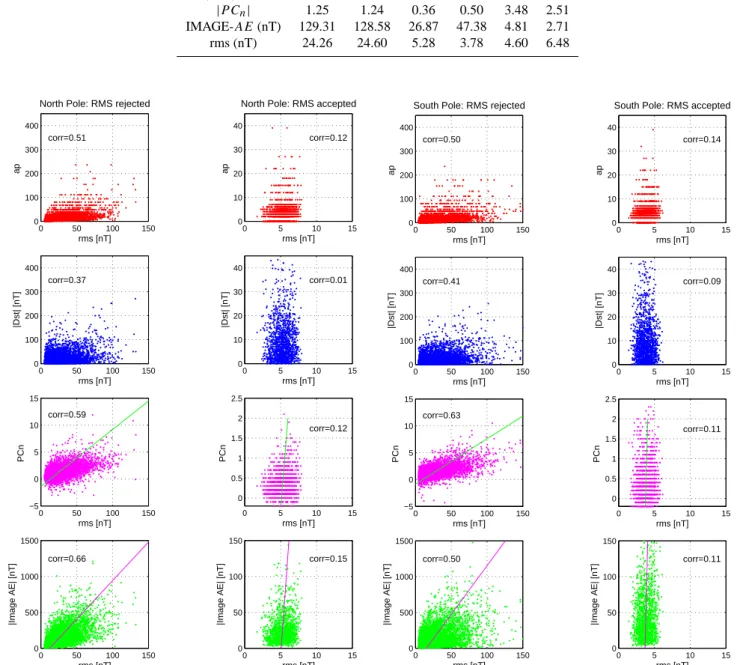
Fig. 2. Correlation analysis between the rms values of the residuals and activity indices ap(Kp), Dst, P Cn, and IMAGE-AE at the north (left) and south pole (right). Left columns for “normal” passes, and in the right columns those accepted by the rms criterion for very quiet orbits. Each diagram shows the index versus the rms value across the polar track, the regression line is added. The correlation coefficients R (“corr”) are listed in the diagrams.
regions (cf. Table 1). Kpalso turns out to represent magnetic
activity at the polar regions not too clearly. Naturally, the
ef-fectiveness of northern based IMAGE-AE and P Cnindices
are reduced at the south pole, but they are still better than Kp
and Dst.
Figure 2 shows the scatter plots of the indices versus the rms values for “normal” and for very quiet passes, and the correlation coefficients R for each distribution. During av-erage activity periods the correlation of the rms values with
0 50 100 150 0 0.1 0.2 0.3 0.4 0.5 IHCs [A/m] corr=0.95 rms [nT]
SOUTH POLE: all
0 50 100 150 0 0.5 1 1.5 2 |FACs| [A/km 2] corr=0.61 rms [nT] (a) 0 5 10 0 0.02 0.04 0.06 0.08
NORTH POLE: quiet
IHCs [A/m] corr=0.18 rms [nT] 0 5 10 0 0.2 0.4 0.6 0.8 |FACs| [A/km 2] corr=0.12 rms [nT] (b) 0 50 100 150 0 0.1 0.2 0.3 0.4 0.5 IHCs [A/m] corr=0.95 rms [nT]
SOUTH POLE: all
0 50 100 150 0 0.5 1 1.5 2 |FACs| [A/km 2] corr=0.61 rms [nT] (c) 0 5 10 0 0.02 0.04 0.06 0.08
SOUTH POLE: quiet
IHCs [A/m] corr=0.23 rms [nT] 0 5 10 0 0.2 0.4 0.6 0.8 |FACs| [A/km 2] corr=0.21 rms [nT] (d)
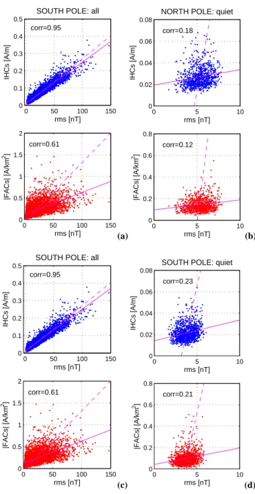
Fig. 3. Correlation analysis between the rms values of the residuals and both the ionospheric Hall and the field-aligned currents deter-mined from CHAMP data at the north (left) and south pole (right). Left columns for “normal” passes, and in the right columns those accepted by the rms criterion for very quiet orbits. The possible range of regression lines is indicated, and the correlation coeffi-cients R (“corr”) are listed in the diagrams.
marginal in both hemispheres. At the north pole the
corre-lation of P Cn with rms is also poor, whereas IMAGE-AE
shows a better but far from good correlation. At the south pole we can observe the opposite case, the correlation of
P Cn with rms is better than that of IMAGE-AE. For the
quiet periods the amplitudes of rms are generally smaller and
for these low rms values none of the indices shows a correla-tion.
The correlations of the ionospheric and field-aligned cur-rents with the rms values is presented in Fig. 3. Since the horizontal currents, as well as the rms values, are computed from the scalar residuals, the correlation coefficients are high for average activity orbits. The FACs amplitudes are signifi-cantly less correlated with rms. The correlation during very quiet periods is not significant for both current systems.
The IMAGE-AE index provided the closest agreement with the rms of the magnetic residuals measured by CHAMP in the north polar region. For this reason we want to explore this index a little further. It has been shown in an earlier study (Ritter et al., 2004) that estimates of the ionospheric Hall cur-rents (IHCs) derived from ground and satellite observations deliver very much the same results when determined from satellite and ground level, above and below the ionosphere. In the subsequent assessment we will consider the physically more meaningful IHCs rather than the rms for the level of magnetic activity.
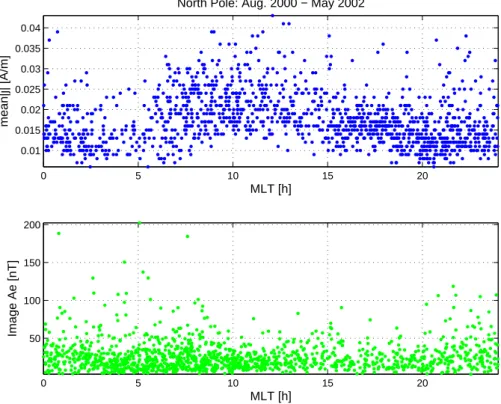
In a first step we compare the variation of the iono-spheric current densities of the quiet orbits as determined by CHAMP with the IMAGE-AE index readings of the times when the satellite passes the northern auroral regions. Fi-gure 4 shows the mean IHC in the top panel and the simulta-neous IMAGE-AE index below. Both are plotted versus the magnetic local time (MLT) of the observations. In case of the IMAGE data the MLT is 2.5 h ahead of UT. For CHAMP results we took the MLT value attained when the satellite crossed the 70◦corrected magnetic (cgm) latitude.
The amplitudes for these quiet passes are fairly low in both panels. Even so, we obtain significantly enhanced cur-rent densities from the satellite data around noon. During the hours 09:00 to 13:00 MLT the amplitudes have almost doubled. The IMAGE-AE gives a slightly different picture. Here we find little dependence on local time except for a shal-low activity minimum around noon.
The observations from CHAMP cover the whole polar re-gions while the IMAGE-AE is derived from a single lon-gitude sector. To study how the quality of the correlation depends on the longitudinal separation of the measurements from ground and space, we re-sampled our results and ex-amine the correlation coefficient of all orbits as a function of magnetic local time difference between the two observations. The result is presented in Fig. 5. As expected, the correlation clearly peaks (>0.8) when the satellite crosses overhead the IMAGE magnetometer network, at the lag time 0. A steep correlation drop can be observed on both sides. For separa-tions of more than 4 h in local time the correlation coefficient varies around 0.6.
The average intensity of the field aligned-currents (FACs) is reduced by a factor of about 3 during the quiet passes com-pared to normal conditions, as can be seen in the bottom row panels of Fig. 3. Besides the reduction in strength there is also a poleward shift of the FACs, and a re-ordering of the upward/downward current pattern takes place. We have cal-culated the current densities of the quiet events according to
0 5 10 15 20 0.01 0.015 0.02 0.025 0.03 0.035 0.04 MLT [h] mean|j| [A/m]
North Pole: Aug. 2000 − May 2002
0 5 10 15 20 50 100 150 200 MLT [h] Image Ae [nT]
Fig. 4. Variation of the ionospheric Hall currents (IHCs) determined from the HAMP scalar residuals (top) and of the IMAGE-AE index (bottom) versus magnetic local time (at 70◦cgm latitude) during very quiet orbits.
−120 −6 0 6 12 0.2 0.4 0.6 0.8 1 corr coef r
North Pole: Aug. 2000 − May 2002
Difference MLT(sat)−MLT(ground) [h]
Fig. 5. Cross correlation analysis between the ionospheric Hall currents (IHCs) determined from CHAMP and the IMAGE-AE index with respect to the difference in magnetic local time for all orbits.
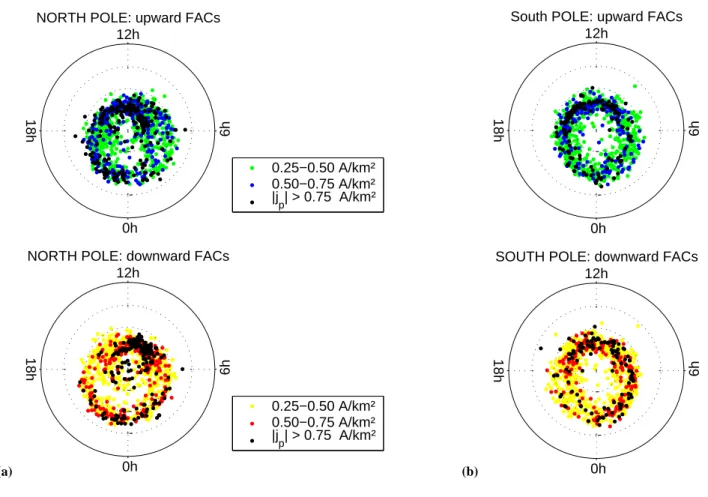
Eq. (1) and then averaged the FAC readings over 20 s, which is equivalent to a spatial average of 135 km at E-region level. Subsequently, we picked the peaks of upward and downward current density of each auroral region pass. The locations of these peaks are plotted in a latitude-magnetic local time frame, using color coding for the different levels of current density.
Figure 6 shows separately the upward and downward FACs both for the north and south poles. Current densities below 0.25 µA/m2 have been omitted from the plots, since they could not be determined reliably. Thus, in ≈30% of the passes across the north pole (≈55% at the south pole), the FAC density was below the measurement threshold.
During these very quiet periods the FAC pattern looks slightly different from normal conditions. The identifica-tion of the Region 1 and 2 currents is not so obvious any longer. When concentrating on the more intense FACs, we find some black dots, denoting the strongest amplitudes in Fig. 6, around midnight. The majority of the high current densities, however, is clustered around noon. Looking at the north pole, intense downward FACs are found in the pre-noon sector, equatorward of the upward FACs, and in the af-ternoon sector, poleward of them. This configuration of FAC pattern is consistent with the results of Stauning et al. (2002) and Vennerstrøm et al. (2002), who studied the distribution of FACs at high latitudes during periods of prolonged northward
(a)
6h
12h
18h
0h
NORTH POLE: upward FACs
0.25−0.50 A/km² 0.50−0.75 A/km² |j p| > 0.75 A/km² 6h 12h 18h 0h
NORTH POLE: downward FACs
0.25−0.50 A/km² 0.50−0.75 A/km² |j p| > 0.75 A/km² (b) 6h 12h 18h 0h
South POLE: upward FACs
6h
12h
18h
0h
SOUTH POLE: downward FACs
Fig. 6. Upward and downward field-aligned currents (FACs) at the north and south poles for quiet periods during the entire time period of this study. Shown are the latitudinal distributions (cgm) of the peak values versus magnetic local time (MLT). The current peaks were determined after applying a 20-s running mean to the 1-s time series. The amplitudes are color coded, with black points representing the strongest peaks in all four panels. The latitude circles are spaced by 10◦cgm.
IMF. Interestingly, the situation is not so clear at the south pole. Here, the FAC distribution looks quite symmetrical around noon. We have no good arguments to explain the hemispheric differences. The FAC intensities, however, are quite similar at both poles.
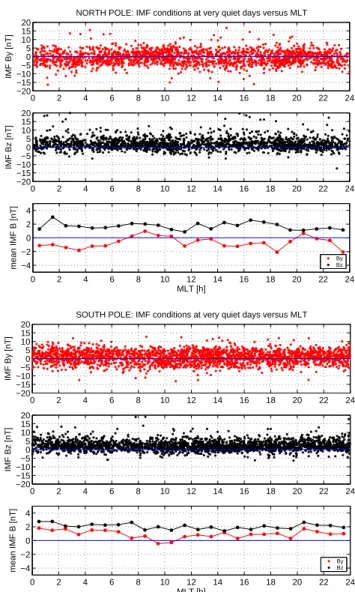
We also considered the interplanetary magnetic field (IMF). When limiting our attention to the quiet time passes we find predominantly positive values for the Bzcomponent,
while By scatters quite evenly about the zero line. In Fig. 7
we plotted the IMF Byand Bzvalues of the quiet times
ver-sus the magnetic local time of the satellite passes, separately for the north and south pole. The two top panels give an im-pression of the encountered values. The bottom panels con-tain averages over one hour in local time. The Bz average
stays close to 2 nT over all times and there is no difference between the hemispheres. Interestingly, we find a slightly negative By average for the north pole samples and a
posi-tive average of similarly small magnitude for the south pole. Since the quiet periods are closely connected to the dark seasons, we may speculate for the investigated time period that a slight tilt of the IMF towards negative Byis favorable
for quiet conditions during the Northern Hemisphere winter,
whereas a small positive By bias seems to allow for quiet
periods during southern winter. This suggestion is supported by a statement in Friis-Christensen and Wilhjelm (1975) who report stronger westward electrojets for IMF By>0 in the
Northern Hemisphere during winter months.
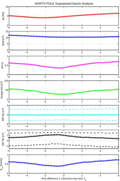
Above, we have tested the correlation between the rms values of the scalar residuals from polar passes and sev-eral magnetic activity indices. In the case of quiet condi-tions no significant correlation was found (cf. Fig. 2). As this might partly be due to a time shift between the reaction of the indices and the polar activity, we performed a super-posed epoch analysis with the various parameters. For each of the quiet passes we defined the closest approach to the magnetic pole as the key time. We determined the respec-tive indices in time segments of ±6 h around the event time, stacked the data of all quiet passes and averaged the compiled index curves at time steps of 10 min.
The results for the north pole are shown in Fig. 8. As ex-pected, the Dst index shows almost no variation over the
whole period. There is a slight decrease in the magnetic activity index, ap, two hours before the key time. Clearer
IMAGE-AE index. Their amplitudes reduce to about 50% some 10–20 min before the key time compared to the levels longer before and after T0. When looking at IMF conditions,
we observe no signature related to the quiet polar region in the Bycomponent. In the Bzcomponent we find a
system-atic positive excursion of the average track surpassing 2 nT. When averaging the positive and negative field readings in-dependently, the positive mean stays constant throughout all hours while the average curve of the negative readings at-tains its smallest values of about −1 nT one hour before the key time.
Another parameter we considered in Fig. 8 is the merging electric field Emas described by Kan and Lee (1979):
Em=vSW
q B2
y+Bz2sin2θ/2 , (2)
where vSWis the solar wind velocity, Byand Bzare the IMF
components and θ is the IMF clock angle. This geoeffective solar wind electric field exhibits a clear minimum shortly be-fore the key time, reaching values below 0.4 mV/m. This quantity seems to be a good indicator for a quiet polar cur-rent system. Results of the superposed epoch analysis for the southern polar region (not shown here) look very much the same.
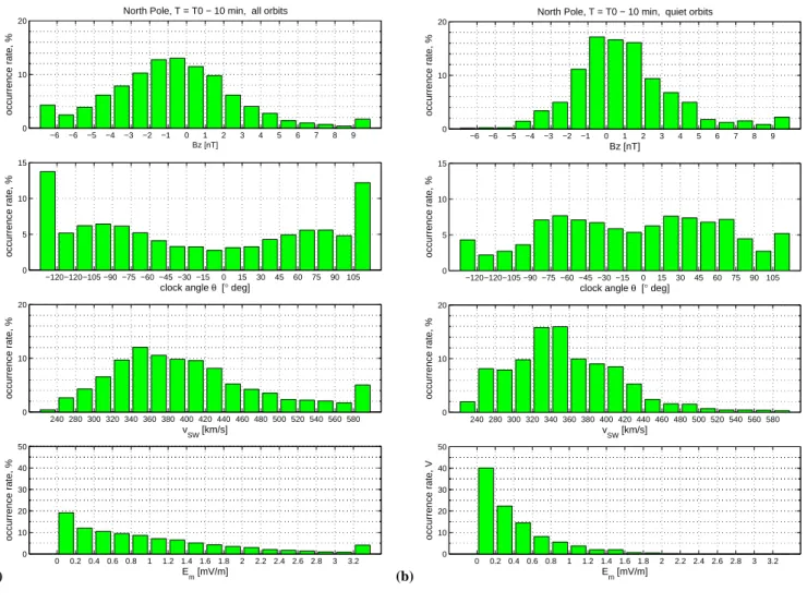
After having realized that the solar wind conditions are a good indicator for auroral activity, equally sensitive for both hemispheres, we carried this a step further. Figure 9 shows the distribution of some solar wind related quantities for all orbits and during the periods which have been identified as quiet in the northern polar region. The following features are found for the quiet periods (right-side histograms): The IMF Bz in the top right panel exhibit a clear positive bias
centered at 1.5 nT. The IMF clock angles in the second frame occur mostly between −90◦and 90◦. The distribution of the solar wind velocity in the third panel peaks at a fairly low speed of 340–360 km/s. Finally, the derived electric field in the bottom frame attains its largest occurrence rate at values less than 0.2 mV/m. From this it becomes quite clear that the merging electric field is a main driver of activity in the high latitude ionosphere.
4 Discussion
We have presented several aspects of the high-latitude iono-spheric current systems during magnetically quiet periods. The events were selected based on the rms value of the vari-ation of the scalar field residuals experienced during the pas-sage of the polar region, beyond 50◦ latitude. Besides the ionospheric currents the crustal anomalies also add to the variations. This is the reason for the different levels of rms values, as observed in Fig. 1, which are, as expected, differ-ent for the two hemispheres. Thus, our rms value also has to be considered as an incomplete measure of the true activity state of the polar ionosphere.
The scalar residuals are only negligibly influenced by field-aligned currents. Their effect is confined to transverse
0 2 4 6 8 10 12 14 16 18 20 22 24 −20 −15 −10 −5 0 5 10 15 20 IMF By [nT]
NORTH POLE: IMF conditions at very quiet days versus MLT
0 2 4 6 8 10 12 14 16 18 20 22 24 −20 −15 −10−5 0 5 10 15 20 IMF Bz [nT] 0 2 4 6 8 10 12 14 16 18 20 22 24 −4 −2 0 2 4 mean IMF B [nT] MLT [h] By Bz 0 2 4 6 8 10 12 14 16 18 20 22 24 −20 −15 −10 −50 5 10 15 20 IMF By [nT]
SOUTH POLE: IMF conditions at very quiet days versus MLT
0 2 4 6 8 10 12 14 16 18 20 22 24 −20 −15 −10 −50 5 10 15 20 IMF Bz [nT] 0 2 4 6 8 10 12 14 16 18 20 22 24 −4 −2 0 2 4 mean IMF B [nT] MLT [h] By Bz
Fig. 7. IMF By and Bz distribution versus magnetic local time (MLT) during quiet polar events. The top frames contain the IMF components taken at the times of the transition between upward and downward FAC peaks for each orbit. The mean values shown in the bottom frames are averaged over 1 h-MLT.
magnetic field components. Also, the Pedersen currents con-tribute little to the magnetic field magnitude (see Ritter et al., 2004), as long as the conductivity gradients are small, which can be expected during quiet periods. We are therefore left with the Hall currents that are responsible for the variations in the obtained rms values. As shown in Fig. 3, the correla-tion coefficient, the rms values, and the Hall current intensity determined from CHAMP data are well beyond 0.9 for both hemispheres. Hence, by using the rms criterion we have se-lected events with weak Hall currents. The amplitudes of rms provide no a priori information on the FAC activity.
The solar zenith angle at the geomagnetic poles turns out to have a strong controlling influence on the occurrence rates of quiet passes (cf. Fig. 1). This is plausible, since the Hall current intensity is the result of the product of the driving electric field and the ionospheric conductivity.
−6 −4 −2 0 2 4 6 0
5 10
ap (Kp)
NORTH POLE Superposed Epoch Analysis
−6 −4 −2 0 2 4 6 0 5 10 15 |Dst| [nT] −6 −4 −2 0 2 4 6 0 0.5 1 |PCn| −6 −4 −2 0 2 4 6 0 50 100 |Image Ae| [nT] −6 −4 −2 0 2 4 6 −5 0 5 IMF By [nT] −6 −4 −2 0 2 4 6 −2 0 2 4 IMF Bz [nT] −6 −4 −2 0 2 4 6 0 0.5 1 Em [mV/m]
time difference ∆ t [hours] to key time T
0
Fig. 8. The Superposed Epoch Analysis reflects the average development of activity indices relative to the time of detection of a quiet polar ionosphere. The parameters (ap, Dst, P Cn, IMAGE-AE, IMF By, IMF Bzand merging electric field Em) are centered at the key time T0,
which is the closest approach of the spacecraft to the geomagnetic pole. The dashed lines in the Bzand Bydiagrams mark the respective negative and positive mean values.
During darkness, the most effective process for enhancing the conductivity is collisional ionisation caused by precipitat-ing electrons. Intense FACs required for this process are gen-erally associated with magnetic storms or substorms. This is the reason why we can classify around 25% of the passes as “quiet” during seasons when the Sun is below the horizon (χ >90◦) at the magnetic pole. On the other hand, hardly any quiet pass is found at summertime, when the polar iono-sphere is continuously sunlit. Then the ever-flowing FACs drive ionospheric currents all the time.
One aim of this study is to find out which of the magnetic indices is best suited to predict the level of activity in the auroral region. There is no single index, as is demonstrated in Sect.3, that is able to identify reliably quiet periods at high latitude. The least suited measure is the storm-time index
Dst. It mainly reflects the ring current intensity. During quiet
times variations of Dst are to be largely caused by the decay
of the ring current. Therefore, this index tracks a current system decoupled from the high latitudes.
The commonly used magnetic activity index Kp or ap
shows a slightly better, but not satisfying relation to the level of activity at high latitudes. Kpis responding to the remote
effects of the auroral electrojets and to variations in the ring current. The polar cap index, P C, reflects the intensity of plasma convection or equivalently the cross-polar cap potential and is thus a lot more effective. With the electric field at high latitude we have already one factor controlling the current intensity. However, for a clear identification of quiet times this is not sufficient.
(a)
−6 −6 −5 −4 −3 −2 −1 0 1 2 3 4 5 6 7 8 9
0 10 20
North Pole, T = T0 − 10 min, all orbits
occurrence rate, % Bz [nT] −120−120−105 −90 −75 −60 −45 −30 −15 0 15 30 45 60 75 90 105 0 5 10 15 occurrence rate, %
clock angle θ [° deg]
240 280 300 320 340 360 380 400 420 440 460 480 500 520 540 560 580 0 10 20 occurrence rate, % v SW [km/s] 0 0.2 0.4 0.6 0.8 1 1.2 1.4 1.6 1.8 2 2.2 2.4 2.6 2.8 3 3.2 0 10 20 30 40 50 occurrence rate, % E m [mV/m] (b) −6 −6 −5 −4 −3 −2 −1 0 1 2 3 4 5 6 7 8 9 0 10 20
North Pole, T = T0 − 10 min, quiet orbits
occurrence rate, % Bz [nT] −120−120−105 −90 −75 −60 −45 −30 −15 0 15 30 45 60 75 90 105 0 5 10 15 occurrence rate, %
clock angle θ [° deg]
240 280 300 320 340 360 380 400 420 440 460 480 500 520 540 560 580 0 10 20 occurrence rate, % v SW [km/s] 0 0.2 0.4 0.6 0.8 1 1.2 1.4 1.6 1.8 2 2.2 2.4 2.6 2.8 3 3.2 0 10 20 30 40 50 occurrence rate, V E m [mV/m]
Fig. 9. Occurrence rates of the IMF Bz, the IMF clock angle θ =atan(By/Bz), the solar wind velocity vSW, and the merging electric field
Emfor all orbits (left) and for the quiet orbits (right), taken at a time t=10 min before the key time. The bars at the left and right ends of the panels include all events occurring beyond the labelled parameter ranges.
In our assessment we have omitted the auroral activity index AE. It is derived from observatories at magnetic lati-tude 65◦to 70◦N. There are two shortcomings with this in-dex. Most of the data for the time interval studied here are still preliminary, and the locations of the stations are too far south to follow the activity properly at very quiet times. As a replacement we tested the IMAGE-AE. This index has the advantage of good latitudinal coverage, but the disadvantage of a limitation to a single longitudinal sector. The compar-ison of the quiet time variations of the ionospheric current densities, as determined by CHAMP with the IMAGE-AE index readings, revealed enhanced current intensities from the satellite data around noon (Fig. 4). Note that there is no event with negligible current density encountered in this time sector. On the other hand, little dependence on local time except for a shallow activity minimum around noon can be observed in the IMAGE-AE index. This discrepancy might be explained by the occurrence of daytime cusp activity at higher latitudes, which is probably missed by the IMAGE
magnetometers, since most of the stations are located fur-ther south. The observed amplitude similarity at nighttime agrees qualitatively with Kauristie et al. (1996), who state a low relative error (less than 20%) between the global AE and the local IMAGE index (AU and AL) during the evening and night hours. A cross-correlation between the IMAGE-AE and CHAMP measurements shows that the auroral activity level is reflected well in the actual sector, but the relation drops off for larger separations (cf. Fig. 5). For time zones more than 4 h apart the correlation coefficient scatters around only 0.6. This analysis gives an indication of the required density of such meridional chains to monitor the auroral ac-tivity globally.
An important quantity controlling the high-latitude pro-cesses is the interplanetary magnetic field (IMF) (Papi-tashvili et al., 2002). We have checked the IMF conditions during our quiet intervals and found, as expected, a predom-inantly positive Bz. The Bycomponent differs only slightly
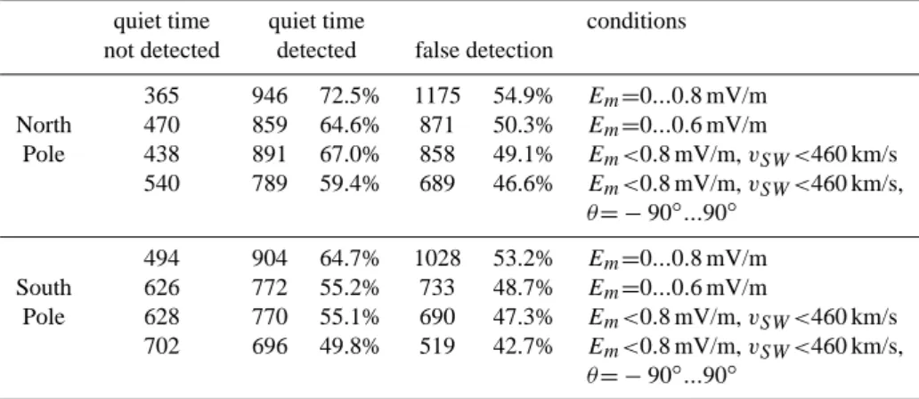
Table 2. Quiet period detection yield for various solar wind conditions.
quiet time quiet time conditions
not detected detected false detection
365 946 72.5% 1175 54.9% Em=0...0.8 mV/m North 470 859 64.6% 871 50.3% Em=0...0.6 mV/m Pole 438 891 67.0% 858 49.1% Em<0.8 mV/m, vSW<460 km/s 540 789 59.4% 689 46.6% Em<0.8 mV/m, vSW<460 km/s, θ = −90◦...90◦ 494 904 64.7% 1028 53.2% Em=0...0.8 mV/m South 626 772 55.2% 733 48.7% Em=0...0.6 mV/m Pole 628 770 55.1% 690 47.3% Em<0.8 mV/m, vSW<460 km/s 702 696 49.8% 519 42.7% Em<0.8 mV/m, vSW<460 km/s, θ = −90◦...90◦
During periods of prolonged northward IMF, reconnection poleward of the cusp starts, and the so-called northward Bz
(NBZ) FAC configuration builds up, which was first outlined by Araki et al. (1984) and Iijima et al. (1984), and later re-fined by Weimer (2001). The distribution of relatively in-tense field-aligned currents in our data, as shown in Fig. 6 (black dots), is consistent with the expected picture in the case of the north pole. We find upward FACs poleward of the downward currents in the pre-noon sector and the opposite sequence on the afternoon side. This pattern is consistent with the detailed studies of Vennerstrøm et al. (2002) and Stauning (2002). These authors also showed that the pre-dicted plasma convection is concentrated around local noon in the case of an NBZ configuration. Our Hall current esti-mates of the quiet orbits show enhanced amplitudes for mag-netic local times between 07:00 and 14:00 MLT (cf. Fig. 4). These observations fit nicely with the expected convection patterns associated with an NBZ configuration. We may therefore conclude that the NBZ-related currents in the day-side cusp and polar cap are the dominating ones during very quiet times and should be taken into account in internal field model approaches.
The superposed epoch analysis is a useful tool to investi-gate the dependence of different parameters. Here, we have tested the delayed response of the auroral activity to the vari-ous indicators. As can be seen from Fig. 8, the apindex goes
through a shallow minimum already 2 h before the key time. It is not clear to us which mechanism is responsible for this delay. The P Cnreaches its minimum 20 min before the key
time. This may be interpreted as the decay time of the auro-ral electrojet. As expected, the IMAGE-AE reacts virtually simultaneously. The ground stations and the satellite respond to the same currents.
In case of the average IMF Bz we obtain a broad
maxi-mum about an hour before the quiet pass. This is valid, al-though the transit time of the signal from ACE satellite to the ionosphere has been taken into account. It has been men-tioned earlier that changes in the solar wind, in particular a switch from negative Bz to positive values may have a
de-layed response of about an hour in the high-latitude convec-tion (Stauning et al., 2003).
After having studied the characteristics of polar current systems during very quiet periods as well as investigating the relation to relevant indices and ambient conditions, we want to make a suggestion for identifying times of quiet condi-tions based on external parameters, e.g. IMF and solar wind velocity. This might be of great interest for magnetic field modelling studies.
As mentioned before, current density is the product of con-ductivity and the electric field. Either one or both have to be small during quiet periods. In general, we can expect low ionospheric conductivity when the Sun is below the horizon. For this reason we limited our interval of predicting low ac-tivity to the times when the magnetic pole is at a zenith angle,
χ >90◦. The obvious second condition is a low electric field as determined by Eq. (2).
In order to test the prediction capability we make a list of all polar passes and single those out which occur during times when our conditions for a quiet period are fulfilled. Then these selected passes are compared with the list of quiet or-bits identified by the rms criterion. The results of this test are compiled in Table 2, separately for the northern and southern polar regions.
When choosing a fairly large range for the electric field, up to 0.8 mV/m, about 2/3 of the quiet passes are captured. More than half of the detections, however, are wrong, i.e. they were not found by the rms criterion. When reducing the E-field range, the false detections become less, but the positive detection yield decreases even faster. In accordance with Fig. 9, we tried to add more constraints on the solar wind conditions. This helped to bring down the false detection rate a little, but again at the expense of positive detections.
The reason for this development is that a good part of the quiet events occur during times of sizable E-fields, stronger than 0.4 mV/m. This requires a very low ionospheric con-ductivity. Since we treat the conductivity as constant over the whole polar region in our approach, it seems to be hard to achieve a reliability of more than 50% in the prediction of
the high-latitude activity state with the help of solar wind
parameters only. A more sophisticated treatment of the
ionospheric conductivity might improve the predictability. Another concern which should be taken into account, is that our activity indicator, the satellite rms value, has its limita-tions, since it responds to both the crustal anomalies and the ionospheric currents. This probably reduces the prediction yield, too.
5 Conclusions
We have studied the features of ionospheric current systems at high magnetic latitudes during quiet times. The domi-nating current distributions encountered, both horizontal and field-aligned, are found to be consistent with the pattern ex-pected for NBZ conditions in the dayside cusp and polar cap region. An important purpose of this study was to find out the prevailing conditions which lead to reduced current intensity. We obtained the following main results:
1. Commonly used activity indices are not well suited for selecting low activity periods of auroral regions. The order of indices from least suitable to best is: Dst, Kp,
P C, IMAGE-AE.
2. The solar zenith angle χ at the magnetic poles has a strong influence on the occurrence rate of quiet events. During the dark polar seasons (χ <90◦), low activity is
encountered at 30% of the satellite passes.
3. A second important factor ruling the ionospheric activ-ity state is the IMF orientation. The majoractiv-ity of the quiet events is accompanied by a positive IMF Bz(0....3 nT).
4. The most suitable indicator of the parameters investi-gated for the detection of low activity periods is a low merging electric field.
5. For the prediction of quiet polar regions a combination of conditions based on the solar zenith angle at the ge-omagnetic poles and the merging electric field are most effective. The success rate ranges around 50% of the events detected by our satellite rms criterion.
For an improvement of the reliability of the predictions a better understanding of the ionospheric conductivity distri-bution is required and probably an enhanced measure for the true polar activity state. This could be the topic of a follow-ing study.
Acknowledgement. The operational support of the CHAMP mis-sion by the German Aerospace Center (DLR) and the financial sup-port for the data processing by the Federal Ministry of Education (BMBF), as part of the Geotechnology Programme, are gratefully acknowledged. We thank the ACE MAG and SWEPAM instrument teams and the ACE Science Center for providing the ACE data. We are obliged to F. Christansen of DMI who kindly provided us with these data propagated to the magnetopause. We thank all institutes maintaining the IMAGE magnetometer network which is the data
base for the IMAGE-AE index. The Dst index data are provided by the WDC-C2 in Kyoto. The P Cnindex is released by the WDC-C1 in Copenhagen. The DFG supported PR through the Priority Programme “Geomagnetic Variations” SPP 1097.
Topical Editor M. Lester thanks L. Cafarella and S. Vennerstr¨om for their help in evaluating this paper.
References
Akasofu, S. I.: Interplanetary energy flux associated with magneto-spheric substorms, Planet. Space Sci., 27, 425, 1979.
Araki, K. T. and Iyemori, T.: Polar cap vertical currents associated with northward interplanetary magnetic field, Geophys. Res. Let-ters, 11, 23–26, 1984.
Bartels, J.: The geomagnetic measures for the time-variations of so-lar corpuscuso-lar radiation, described for use in correlation studies in other geophysical fields, Ann. Intern. Geophys. Year, 4, 227– 236, 1957.
Baumjohann, W. and Treumann, R. A.: Basic Space plasma Physics, Imperial College Press, London, 47–72, 1996. Campbell, W.: Introduction to geomagnetic fields, Cambridge
Uni-versity Press, 1997.
Friis-Christensen, E. and Wilhjelm, J.: Polar cap currents for dif-ferent directions of the interplanetary magnetic field in the Y-Z plane, J. Geophys. Res., 80, 1248, 1975.
Hirshberg, J. and Colburn, D. S.: Interplanetary field and geomag-netic variations: A unified view, Planet. Space Sci, 17, 1183, 1969.
Holme, R., Olsen, N., Rother, M., and L¨uhr, H.: CO2 – A CHAMP magnetic field model, “First CHAMP Mission Results for Grav-ity, Magnetic and Atmospheric Studies”, edited by Reigber, C., L¨uhr, H., and Schwintzer, P., Springer, Berlin, 220–225, 2003. Iijima, T., Potemra, T. A., Zanetti, L. J., and Bythrow, P. F.:
Large scale Birkeland currents in the dayside polar region dur-ing strongly northward IMF: a new Birkeland current system, J. Geophys. Res., 89, 7441–7452, 1984.
Kan, J. R. and Lee, L. C.: Energy coupling function and solar wind – Magnetosphere dynamo, Geophys. Res. Lett., 6, 577, 1979. Kauristie, K., Pulkkinen, T. I., Pellinen, R. J., and Opgenoorth, H.
J.: What can we tell about global-auroral electrojet activity from a single meridionial magnetometer data chain?, Ann. Geophys., 14, 1177–1185, 1996.
Kerz, W.: Ring current variations during the IGY, Ann. Int. Geo-phys. Year, 35, 49, 1964.
L¨uhr, H., Warnecke, J., and Rother, M.: An algorithm for estimat-ing field-aligned currents from sestimat-ingle spacecraft magnetic field measurements: a diagnostic tool applied to Freja satellite data, IEEE Trans Geosci. Remote Sens., 34, 1369–1376, 1996. Maus, S., Rother, M., Holme, R., L¨uhr, H., Olsen, N., and Haak, V.:
First scalar magnetic anomaly map from CHAMP satellite data indicates weak lithospheric field, Geophys. Res. Lett., 29, (14), doi:10.1029/2001GL013685, 2002.
Olsen, N.: A new tool for determining of ionospheric currents from satellite data, Geophys. Res. Lett., 23, 3635–3638, 1996. Olsen, N.: A model of the geomagnetic main field and its secular
variation for epoch 2000 estimated from Ørsted data, Geophys. J. Int., 149, 454–462, 2002.
Papitashvili, V. O., Christiansen, F., and Neubert, T.: A new model of field-aligned currents derived from high-precision satellite magnetic field data, Geophys. Res. Lett., 29, (14), doi:10.1029/2001GL01420, 2002.
Papitashvili, V. O., Gromova, L. I., Popov, V. A., and Ras-mussen,O.: Northern Polar Cap magnetic activity index PCN: Effective area, universal time, seasonal and solar cycle varia-tions, Scientific Report 01-01, Danish Meteorological Institute, Copenhagen, Denmark, 57, 2001.
Ritter, P., L¨uhr, H., and Maus, S.: The polar current system at very quiet times, in OIST-4 Proceedings, edited by Stauning, P., L¨uhr, H., Ultr´e-Gu´erard, P., LaBreque, J., Purucker, M., Primdahl, F., Joergenson, J., Christiansen, F., Hoeg, P., and Lauritsen, K., 189, DMI, Copenhagen, 2003.
Ritter, P., L¨uhr, H., Viljanen, A., Amm, O., Pulkkinen, A., and Sil-lanp¨a¨a, I.: Ionospheric currents estimated simultaneously from CHAMP satellite and IMAGE ground-based magnetic field mea-surements: A statistical study at auroral latitudes, Ann. Geo-phys., 22, 417–430, 2004.
Siebert, M.: Maßzahlen der erdmagnetischen Aktivit¨at, “Handbuch der Physik”, Springer, Heidelberg, vol. 49, (3), 206–275, 1971. Sillanp¨a¨a, I., L¨uhr, H., Viljanen, A., and Ritter, P.: Quiet-time
Mag-netic Variations at High Latitude Observatories, Earth Planets Space, vol. 56(1), 39–45, 2004.
Stauning, P.: Field-aligned ionospheric current systems observed from the Magsat and Ørsted satellites during northward IMF, Geophys. Res. Lett., 29, doi:10.1029/2001GL013961, 2002. Stauning, P., Christiansen, F., Watermann, J., Christensen, T., and
Rasmussen, O.: Mapping of Field aligned current patterns dur-ing northward IMF, “First CHAMP Mission Results for Gravity, Magnetic and Atmospheric Studies”, edited by Reigber, C., L¨uhr, H., and Schwintzer, P., Springer, Berlin, 353–362, 2003. Sugiura, M.: Hourly values of equatorial Dst for the IGY, Ann. Int.
Geophys. Year, 35, 9–45, 1965.
Sugiura, M. and Kamei, T.: Equatorial Dst index, 1957–1986, IAGA Bulletin, edited by Berthelier, A. and Menvielle, M., ISGI Publ. Off. Saint Maur, vol. 40, 1991.
Troshichev, O. A., Andrezen, V. G., Vennerstrøm, S., and Friis-Christensen, E.: Magnetic activity in the polar cap – A new in-dex, Planet. Space Sci., 36, 1095, 1988.
Vennerstrøm, S. and Friis-Christensen, E.: Comparison between the polar cap, PC, and the auroral electrojet indices AE, AL, and AU, J. Geophys. Res., 96, (A1), 101–113, 1991.
Vennerstrøm, S., Friis-Christensen, E., Troshichev, O. A., and Andrezen, V. G.: Geomagnetic Polar Cap (PC) Index 1975– 1993, Report UAG-103, WDC-A for Solar-Terrestrial Physics, NOAA/NGDC, Boulder, Colorado, 274, 1994.
Vennerstrøm, S., Moretto, T., Olsen, N., Friis-Christensen, E., Stampe, A., M., and Watermann, J. F.: Field-aligned currents in the dayside cusp and polar cap region during northward IMF, J. Geophys. Res., 107, (A8), doi:10.1029/2001JA009162, 2002. Weimer, D. R.: Models of high-latitude electric potential derived
with a least-error fit of spherical harmonic coefficients, J. Geo-phys. Res., 100, 595, 1995.
Weimer, D. R.: Maps of ionospheric field-aligned currents as a function of the interplanetary magnetic field derived from Dynamics Explorer 2 data, J. Geophys. Res., 106, (A7), doi:12.889/2000JA000295, 2001.
Weimer, D. R., Ober, D. M., Maynard, N. C., Collier, M. R., McCo-mas, D. J., Ness, N. F., Smith, C. W., and Watermann, J.: Predict-ing interplanetary magnetic field (IMF) propagation delay times using the minimum variance technique, J. Geophys. Res., 108, (A1), doi:10.1029/2002JA009405, 2003.
Xu, W.-Y.: Polar region Sq in quiet daily geomagnetic fields, 317– 393, 1989.