HAL Id: hal-03007840
https://hal.archives-ouvertes.fr/hal-03007840
Preprint submitted on 16 Nov 2020
HAL is a multi-disciplinary open access
archive for the deposit and dissemination of
sci-entific research documents, whether they are
pub-lished or not. The documents may come from
teaching and research institutions in France or
abroad, or from public or private research centers.
L’archive ouverte pluridisciplinaire HAL, est
destinée au dépôt et à la diffusion de documents
scientifiques de niveau recherche, publiés ou non,
émanant des établissements d’enseignement et de
recherche français ou étrangers, des laboratoires
publics ou privés.
A. Noullez
To cite this version:
A. Noullez. Turbulence Homogeneity and Isotropy : Mean-field and Fluctuations in the Taylor-Green
vortex. 2020. �hal-03007840�
Journal: Journal of Fluid Mechanics Manuscript ID Draft
mss type: JFM Papers Date Submitted by the
Author: n/a
Complete List of Authors: NOULLEZ, Alain; CNRS, Observatoire de la Cote d'Azur
Keyword: Homogeneous turbulence < Turbulent Flows, Isotropic turbulence < Turbulent Flows, Turbulence simulation < Turbulent Flows
Abstract:
We have performed medium resolution numerical simulations over very long times of the stationary turbulent flow that develops from a static constant in time Taylor-Green forcing. By averaging over thousands of large-scale eddy turnover times, we separate the turbulent fluctuations from the inhomogeneous anisotropic mean flow induced by the forcing. We show that the turbulent velocity fluctuations are only slightly more isotropic than the total flow and still display significant deviations from isotropy and homogeneity. Also, the fluctuations and the mean flow are not independent, and their energies are locally anticorrelated. The energy transfer laws of Kolmogorov, Yaglom and Monin and their corresponding finite Reynolds number corrections are also checked for different positions and orientations in the flow, and it is found that Kolmogorov and Yaglom laws are not completely satisfied due to the imperfect return to isotropy and homogeneity of the flow. Monin's relation is verified because it averages dissipation over the different directions and in a volume such that homogeneity is restored, and also only for the total fluid velocity and not for the velocity fluctuations as these do not obey Navier-Stokes equations. These results suggest that the hypothesis of small scale homogeneous and isotropic turbulence should be clarified in the presence of an inhomogeneous anisotropic mean flow induced by forcing.
Turbulence Homogeneity and Isotropy :
Mean-field and Fluctuations in the
Taylor-Green vortex
Alain Noullez†
Universit´e Cˆote d’Azur, Observatoire de la Cˆote d’Azur, CNRS, Laboratoire Lagrange, bd. de l’Observatoire, C.S. 34229, 06304 Nice Cedex 4, France
(Received xx; revised xx; accepted xx)
We have performed medium resolution numerical simulations over very long times of the stationary turbulent flow that develops from a static constant in time Taylor-Green forcing. By averaging over thousands of large-scale eddy turnover times, we separate the turbulent fluctuations from the inhomogeneous anisotropic mean flow induced by the forcing. We show that the turbulent velocity fluctuations are only slightly more isotropic than the total flow and still display significant deviations from isotropy and homogeneity. Also, the fluctuations and the mean flow are not independent, and their energies are locally anticorrelated. The energy transfer laws of Kolmogorov, Yaglom and Monin and their corresponding finite Reynolds number corrections are also checked for different positions and orientations in the flow, and it is found that Kolmogorov and Yaglom laws are not completely satisfied due to the imperfect return to isotropy and homogeneity of the flow. Monin’s relation is verified because it averages dissipation over the different directions and in a volume such that homogeneity is restored, and also only for the total fluid velocity and not for the velocity fluctuations as these do not obey Navier-Stokes equations. These results suggest that the hypothesis of small scale homogeneous and isotropic turbulence should be clarified in the presence of an inhomogeneous anisotropic mean flow induced by forcing.
Key words:
1. Introduction
Homogeneous and Isotropic Turbulence (HIT) is one of the most useful concepts for the study and characterization of fluid turbulence. This paradigm is based on the hypothesis (or postulate) that, far away from any boundary and at sufficiently small scales, turbu-lence ‘forgets’ about initial conditions and forcing mechanism and its statistical properties do not depend anymore on position or orientation. This implies in particular that two-point statistical quantities are functions only of the modulus of the distance between them and allows the description of turbulence through the energy spectrum, correlation function or structure functions, and many properties of these can be obtained only by using arguments of isotropy and incompressibility (see among others Hinze (1959), Monin & Yaglom (1975) or Frisch (1995)). The hypothesis of HIT at small scales is reasonably confirmed experimentally at sufficiently high Reynolds number Re for anisotropic (but homogeneous) shear flows when the shear rate is small (see e.g. Kim & Antonia (1993)
or Antonia & Kim (1994)), and of course numerically with homogeneous and isotropic volume forcing without boundaries (e.g. turbulence in a periodic box like in Gotoh, Fukayama & Nakano (2002)). It is however not clear if and how well it can be verified in the case of a strongly anisotropic and inhomogeneous volume or boundary forcing, which is often the case in experimental studies, like for instance the von K´arm´an swirling flow that has often been used recently to obtain very turbulent flows (high Re) in a small volume (Douady, Couder, & Brachet (1991); Monchaux, Ravelet, Dubrulle, Chiffaudel & Daviaud (2006); Ravelet, Chiffaudel & Daviaud (2008)). Indeed, even at very high Reynolds number Re, such forcing lead to a nonzero mean flow, often with topologies more complex than the forcing itself, that leaves a non-homogeneous anisotropic imprint on the total turbulent flow. As an example, (Huck, Machicoane & Volk 2017) recently studied the turbulence close to the central stagnation point in the von K´arm´an flow and found it to be strongly anisotropic and inhomogeneous, even at Re ≈ 27000 (Rλ≈ 225).
One of the aims of this paper is to investigate these deviations from HIT in the case of a numerical Taylor-Green flow, the simplest numerical equivalent of the von K´arm´an swirling flow. The advantage of using numerical simulations is that we can compute easily all longitudinal and transverse structure functions of the flow, and check the isotropic predictions for them, while measuring these quantities experimentally is a much more complex task. Also, the Taylor-Green vortex has been mostly studied in the spectral wavenumber space, with or without invoking global anisotropy (Brachet, Meiron, Nickel, Morf & Frisch 1983), but studies in physical space using correlations or structure functions are scarse, probably because of the high computational cost, while measurements in the von K´arm´an flow have been done only in physical space. It is thus interesting to try to relate these measurements and bridge the gap between these two flows using a common representation.
Another common idea in turbulence is that, in the presence of a mean flow due to the forcing mechanism, the turbulent fluctuations with respect to the mean flow will be much closer to HIT than the total flow. This leads to the image of homgeneous and isotropic fluctuations living independently of a mean static anisotropic and inhomoge-neous background. This image was however recently contradicted by (Huck, Machicoane & Volk 2017) who found both mean flow and turbulent fluctuations to be inhomogeneous and anisotropic. Moreover, exchange of energy between man flow and fluctuations was oberved. In order to investigate this idea, we decided to perform very long simulations of the Taylor-Green flow (thousands of eddy turnover times), so that we can extract the mean flow by time averaging and study separately the turbulent fluctuations around the mean flow. Our goal was to check whether these are in fact spatially independent of the mean flow (that is indeed strongly anisotropic and inhomogeneous), and a better realisation of HIT than the total flow itself.
One of the most important results in the theory of stationary HIT is Kolmogorov’s equation −D[∆ui(ri)] 3E + 6 ν ∂i D [∆ui(ri)] 2E =4 5 ε |ri| , (1.1)
relating the average cube of the longitudinal velocity increments ∆ui(ri) ≡ ui(x + ri) −
ui(x) in any direction ri ≡ r 1i and the mean energy dissipation rate in the flow
ε ≡ −dE dt = ν |∇u|2® = ν |∇ × u|2® = 1 2ν * X i,j µ ∂ui ∂xj +∂uj ∂xi ¶2+ , (1.2)
obtained by Kolmogorov in 1941 (Kolmogorov 1941), starting from the K´arm´an-Howarth equation (K´arm´an & Howarth 1938). In the limit of zero viscosity, (1.1) reduces to the
celebrated Kolmogorov ‘four-fifth’ law D [∆ui(ri)] 3E = −4 5 ε r , (1.3)
important because it is both ‘exact and non-trivial’ (Frisch 1995). Kolmogorov’s equation is derived exactly only under the hypothesis of global homogeneity and isotropy (Frisch 1995), but support has been given for its validity even for anisotropic turbulence (e.g. Monin & Yaglom (1975)). It is thus interesting to verify if it could be satisfied also in the presence of an inhomogeneous anisotropic mean flow, like the von K´arm´an flow. This is what we will do in this paper, checking the validity of (1.1) at different locations and for different directions of our numerical Taylor-Green flow. Of course, in that case, it is very important to define the meaning of that averaging h. . .i operation.
Monin (Monin 1959) tried to establish Kolmogorov’s equation (1.1) under less restric-tive conditions, working from the start with velocity increments rather than velocity correlations to establish an equivalent of the K´arm´an-Howarth equation for velocity increments. This approach was later examined again and extended by (Antonia, Ould-Rouis, Anselmet & Zhu 1997), (Hill 1997) and (Danaila, Anselmet, Zhou & Antonia 2001) to obtain another more general form of (1.1),
−|∆u(ri)| 2 ∆ui(ri)®+ 2 ν ∂i|∆u(ri)| 2® =4 3 ε r , (1.4)
i.e. a ‘four-third’ law that we will refer from now on as Yaglom’s law (even if it was never written by Yaglom) because, as noted by (Antonia, Ould-Rouis, Anselmet & Zhu 1997), it is exactly analogous to Yaglom’s equation for the transport of temperature increments by turbulence (Yaglom 1949). Yaglom’s equation has however an important difference with Kolmogorov’s equation in that its derivation does not require global but only local isotropy (Hill 1997) and represents an extended form (over all velocity components) of Kolmogorov’s equation. An even more general relation was obtained by (Monin 1959)
−∇ ·|∆u(r)|2
∆u(r)®+ 2 ν ∇2
|∆u(r)|2®
= 4 ε , (1.5)
that, following (Hill 1997), we’ll call Monin’s law and only requires the assumption of homogeneity for its derivation (Hill 1997) without the need for isotropy, and is thus the most general relation that can be obtained between the energy dissipation and the third-order velocity vector structure function, valid even for anisotropic turbulence.
Yaglom’s law (1.4), and even more Monin’s law (1.5), are not very well-known in the turbulence community, probably because they are much harder to study experimentally, the former requiring the measurement of all velocity components in a given direction and the latter requiring all velocity components in all directions, while Kolmogorov’s law (1.1) only requires one velocity component in one direction, so that it is relatively easy to measure using for example hot-wire probes. Experimental verifications of Yaglom’s law have been performed by (Antonia, Ould-Rouis, Anselmet & Zhu 1997) and (Danaila, Anselmet, Zhou & Antonia 2001), while (Lamriben, Cortet & Moisy 2011) observed Monin’s law in anisotropic axisymmetric rotating turbulence. Yaglom’s law and Monin’s law are however very important, not only because they require less restrictive isotropy or homogeneity constraints than Kolmogorov’s law, but also because they are more general and can be extended to the transport of other quantities by an incompressible velocity field (e.g. the transport of temperature by turbulence originally considered by Yaglom (1949)). Yaglom’s equation has for instance be generalised to MHD turbulence by (Politano & Pouquet 1998), (Politano & Pouquet 1998) for the transport of the two Els¨asser fields z±
used by (Sorriso-Valvo, Marino, Carbone, Noullez, Lepreti, Veltri, Bruno, Bavassano, & Pietropaolo 2007), (Marino, Sorriso-Valvo, Carbone, Noullez, Bruno & Bavassano 2008) to measure the turbulent energy cascade dissipation rate in the Solar wind. The Solar wind is however not perfectly homogeneous nor isotropic, and it is not clear how sensitive Yaglom’s law or Monin’s law are sensitive to these effects. So we decided to also check both of these laws in our Taylor-Green flows, along with Kolmogorov’s law to establish which, if any, of these can be trusted in the presence of inhomogeneities or anisotropies in the mean flow, for both the total flow and the fluctuations. Once again, we repeat that the whole study will be performed by computing structure functions in physical space along different spatial directions, without invoking isotropy from the start. Numerical verifications of energy transfer laws, or of the homogeneity and isotropy of turbulence at small scales are not common in the litterature, and one of the few examples is the very interesting work of (Gotoh, Fukayama & Nakano 2002) who showed that at sufficiently high Reynolds numbers, isotropy at small scales is well verified and that Kolmogorov and Yaglom laws are statisfied if the viscous correction is taken into accound (Monin’s law was not considered). However, the authors used an isotropic random white in time forcing for which the mean flow is zero and the statistical properties of the flow are homogeneous by construction, so it is interesting to reproduce that study with the TG forcing.
Our paper is organised as follows. In section 2, we present a brief derivation of Yaglom’s law (1.4) and Monin’s law (1.5) for people who are not familiar with these, and also to clarify our notations and emphasise the hypotheses that are used at various steps of the derivation for both laws. Section 3 describes the numerical flow and our Taylor-Green forcing, and gives all numerical parameters and global measurements of the simulation. In section 4, we precise all averaging procedures that we used, both to get the mean flow and to measure one-point and two-point statistical quantities in all directions, either in the whole volume or in specific planes. Results for the statistical homogeneity and isotropy at second order, both in one point or through the use of second order longitudinal or transverse structure functions are presented in section 5. The validity of Kolmogorov’s law, Yaglom’s law and Monin’s law is investigated in section 6. In the concluding section 7, we discuss about the implications of our results on the measurement of energy transfer laws in flows with a non trivial mean flow due to non-homogenous anisotropic forcing.
2. Energy transfer laws
Our derivation of energy transfer laws (1.1), (1.4) and (1.5) completely follows (Anto-nia, Ould-Rouis, Anselmet & Zhu 1997) and (Danaila, Anselmet, Zhou & Antonia 2001), so we will be brief, refering to these two papers for details and to (Hill 1997) and (Monin & Yaglom 1975) for the precise statement of the homogeneity and isotropy conditions for random vectors (not necessarily solutions of the Navier-Stokes equations). We will try to use vector notation throughout that, besides being much more concise, has (we believe) the advantage of being less ambiguous.
We start with the incompressible Navier-Stokes equation ∂tu′+ u′· ∇x′u ′ = ∇x′p ′ + ν ∇2 x′u ′ + f′ (2.1) ∂tu+ u · ∇xu= ∇xp + ν ∇ 2 xu+ f (2.2)
written at two points x and x′
≡ x + r separated by r, for the two velocities u′
(x′
) and u(x), p and p′
are the kinematic pressure per unit mass, and ∇x and ∇ 2 x are
respectively the gradient and laplacian with respect to the x (or x′
) coordinates. We then subtract the equation written at x from the equation at x′
the velocity increment
∆u(r; x, t) ≡ u(x + r, t) − u(x, t) . (2.3) We emphasise that the difference operator ∆ does not change the vectorial or scalar character of its argument and that, applied to a vector, it yields a vector and gives a scalar when applied to a scalar. We then multiply the time evolution equation for the velocity increment by the velocity increment itself 2 ∆u and average on spatial locations x to get ∂t|∆u|2®+ ∇r· |∆u|2 ∆u®= 2 ν ∇2 r |∆u|2® − 4 ν |∇u|2® + 2 h∆f · ∆ui . (2.4) Here, local homogeneity has been used multiple times to (1) rewrite differential oper-ators with respect to x or x′ after averaging in terms of derivatives with respect to r:
∇x′ = −∇x= ∇r; (2) eliminate of the pressure-velocity correlations (see Hill (1997)).
Incompressibility has also been used. The first term on the l.h.s. of (2.4) is the rate of change of the velocity increment variance at scale r, that at large scales should go to four times the rate of change of the energy ε (1.2). Order of magnitude arguments show that this non-stationary term should become small when the separation becomes small, going like (r/L)2/3 and thus can be neglected at small scales. Alternatively, we can consider
stationary turbulence and average over time to eliminate the time-fluctuating term. The forcing term will also disappear at small scales if the force f is regular in space and concentrated at large scales. With these simplifications, (2.4) becomes
∇r· |∆u(r)|2 ∆u(r)®= −4 ε + 2 ν ∇2 r |∆u(r)|2® , (2.5)
which is Monin’s equation (1.5) using the definition of the mean energy dissipation rate (1.2). Only homogeneity and stationarity have been used to obtain this relation, but it is important to note the meaning of the averaging operator h. . .i that we used: we have to average in space x over scales such that the quantities defined in (2.5) are independent of x (homogeneous). Also, we have to average over times such that the time-derivative term can be neglected.
Written in the form (1.5), Monin’equation appears as a scale-by-scale dissipation budget equation. The r.h.s. of (1.5) is the total dissipation 4 ε, that is (four times) the energy that disappears at any scale, and has to be constant across scales if a stationary state is reached. It is made up of the two terms on the l.h.s. of (1.5) which are both positive for three-dimensional turbulence. The first term ∇ ·|∆u(r)|2
∆u(r)®represents the energy that is transfered to smaller scales by the turbulent advection, while the second term 2 ν ∇2
|∆u(r)|2®
is the energy dissipated at each scale by the molecular viscosity. At very small scales and for finite viscosity, the flow is regular and the transfer term becomes negligible, so that we can compute the dissipation from the total second-order structure function ε = 1 2ν limr→0∇ 2 |∆u(r)|2® , (2.6)
which is equivalent to (1.2), and is valid for homogeneous anisotropic turbulence. On the other hand, for small viscosities at intermediate inertial scales or in the limit of vanishing viscosity, we have
∇ ·|∆u(r)|2∆u(r)®= −4 ε , (2.7)
that provides a route for energy to be dissipated (in fact, transfered to smaller scales) at all scales, even for a vanishing viscosity, and is the anisotropic generalisation of Kolmogorov ‘four-fifth’ law (1.3). It implies that the energy flux vector
F(r) ≡|∆u(r)|2
has a negative divergence ∇ · F = −4 ε, so that energy is transfered by the turbulent advection towards the small scales.
If we now assume local isotropy and project equation (2.5) on any direction ri, the
only non-singular solution of the scalar equation that results is |∆u(ri)| 2 ∆ui(ri)®= − 4 3 ε r + 2 ν ∂i |∆u(ri)| 2® , (2.9)
with ∂i≡ ∂/∂ri, or (in vector form)
|∆u(r)|2 ∆u(r)®= −4 3 ε r + 2 ν ∇r |∆u(r)|2® , (2.10)
that is, Yaglom’s law (1.4). Once again, (1.4) is a conservation law, but for the total dissipation integrated from 0 to r, and that has to linearly proportional to r if the total dissipation itself (1.5) is independent of scale. Local isotropy then implies that the energy flux vector (2.8) and the velocity increment variance are purely radial functions, so that we have in the limit of vanishing viscosity or in the inertial range a negative energy flux vector
F(r) =|∆u(r)|2
∆u(r)®= −4
3 ε r (2.11)
showing that the energy is transfered from large to small scales by the turbulence. By differentiating (1.4) at small scale, we also have a definition of the dissipation valid for homogeneous and locally isotropic flows
ε = 3 2ν limr→0∂ 2 i |∆u(ri)| 2® = 3 ν lim r→0 |∆u(ri)|2® r2 = 3 ν * X j µ∂u j ∂xi ¶2+ . (2.12) To get Kolmogorov’s equation (1.1) from Yaglom’s law (2.9), we need to use relations valid for globally isotropic incompressible turbulence (see Monin & Yaglom (1975), Hinze (1959) or Hill (1997)) D [∆uj(ri)] 2 ∆ui(ri) E = 1 3 D [∆ui(ri)] 3E j 6= i , (2.13)
valid in the inertial range, and D [∆uj(ri)] 2E = 2D[∆ui(ri)] 2E j 6= i , (2.14)
valid at small scales, to finally obtain equation (1.1) and also a definition of the dissipation that can be measured using only longitudinal increments of the velocity
ε = 15 2 ν limr→0∂ 2 i D [∆ui(ri)] 2E = 15 ν lim r→0 D [∆ui(ri)] 2E r2 = 15 ν *µ ∂ui ∂xi ¶2+ , (2.15) but is valid only for homogeneous globally isotropic turbulence. Kolmogorov’s equation, whilst very important, is thus less general than either (1.4) and (1.5), requiring a priori not only homogeneity, but also global isotropy of the flow for its derivation. It is thus particularly interesting to investigate experimentally or numerically the validity of these three laws in a flow which is stongly anisotropic and inhomogeneous at large scales, and this is what we will try to perform in the rest of this paper, for the Taylor-Green vortex flow.
0 π
π
2π 2π
Figure 1.The Taylor-Green vortex forcing consists of two counter-rotating vortices replicated antisymmetrically two times in each direction to obtain a 2π-periodic tridimensional flow consisting of eight coupled swirling flow cells. The forcing consists of both differential rotation (planes z = kπ have maximal rotational forcing) and pure shear (forcing is zero in the planes z = π/2 + kπ).
3. The numerical Taylor-Green flow
The numerical flow that we use is the Taylor-Green (TG) vortex flow, orig-inally introduced by (Taylor & Green 1937) to study the generation of small scales and turbulence by vortex stretching in the Navier-Stokes equations. It is defined as the flow that develops from the initial conditions u(x, y, z, 0) ≡ (sin(k0x) cos(k0y) cos(k0z), − cos(k0x) sin(k0y) cos(k0z), 0)T (see figure 1 for k0 = 1),
following the unforced incompressible Navier-Stokes equations (2.2) with f ≡ 0. As we want to study stationary turbulence , we will add a constant forcing term identical to the initial conditions
f(x, y, z) = 2 frms
sin(k0x) cos(k0y) cos(k0z)
− cos(k0x) sin(k0y) cos(k0z)
0
, (3.1)
to be able to reach a state statistically stationary in time. Note that this is a large scale constant in time volume forcing while the von K´arm´an swirling flow uses forcing at the boundaries. Still, these two flows share many properties like a strong rotation and an inhomogeneous forcing amplitude along the z-axis. It should also be noted that, even if the forcing amplitude frms is kept constant in time, because the velocity field u(x, t)
is fluctuating in time, both the instantaneous power injection hf · ui, the instantaneous power dissipation ε(t) and the total energy E(t) ≡ u2®
/2 are fluctuating in time. It is only after averaging in time that injection and dissipation are equal, and that the energy is constant. The original (decaying) Taylor-Green vortex has been extensively
N3 ⇐ 1283 L ≡ 2π Λ = 2.589 λ = 0.487 η = 0.035 ∆x ⇐ 0.049 frms⇐ 1.5 Urms= 2.69 E = 3.62 ˙|∇U | 2 ¸ = 150.5 Ω = 75.2 ν ⇐ 0.015 Re= 440 Rλ= 85 ε = 2.257 ∆t ⇐ 1 Tnl= 0.961 dt ⇐ 10− 3 Nt⇐ 2 × 10 3
Table 1.Numerical parameters of our simulation runs of the forced Taylor-Green parameters. Values marked with ⇐ are set initially at the beginning of the run, while those marked with = are controlled by the time evolution and measured during the simulation. L is the size of the box, Λ is the flow integral scale 3π/4 [R dk E(k)/k]/E, λ is the Taylor scale {5E/[R dk k2
E(k)]}1/2= (5E/Ω)1/2, η is the Kolmogorov scale (ν3
/ε)1/4and ∆x ≡ 2π/N
is the simulation gridsize. dt is the simulation timestep, Tnl is the eddy turnover time Λ/Urms
and ∆t is the time separation between each of the Nt samplings of the velocity field for time
averaging.
studied numerically since the advent of digital computers (e.g. Brachet, Meiron, Nickel, Morf & Frisch (1983) and references therein) and has been found to become turbulent already at rather small Reynolds numbers. The stationary forced Taylor-Green vortex has been extensively used as a prototype flow to study dynamo action in MHD flows driven by the von K´arm´an swirling flow (e.g. Nore, Brachet, Politano & Pouquet (1997), Ponty, Mininni, Montgomery, Pinton, Politano & Pouquet (2005) and Ponty, Mininni, Pinton, Politano & Pouquet (2007)), but studies of the statistical properties of the hydrodynamical TG vortex in the space domain through the use of structure functions are relatively uncommon. One of the few examples is (Mininni, Alexakis & Pouquet 2008) where structure functions were used to study intermittency, but the authors only considered longitudinal structure functions averaged in the x and y directions, and used absolute values for odd orders and extended self-similarity to improve the scaling. Energy transfer laws, isotropy and homogeneity were thus not considered in that work that rather concentrated on the inter-mode energy transfers assuming isotropy.
For all values of (integer) wavenumber k0, the Taylor-Green vortex is known to have
many symmetries that are dynamically compatible with the Navier-Stokes and that are thus preserved by the time evolution if both initial conditions and forcing satisfy these symmetries (Brachet, Meiron, Nickel, Morf & Frisch 1983). This can be used to build an optimised pseudospectral code that implements directly all these symmetries so that they are preserved exactly by the code at all times, reducing memory and computational burden by a factor of 64 (Nore, Brachet, Politano & Pouquet 1997), but producing eight symmetrically replicated correlated realisations of the flow. However, the TG symmetries can be spontaneously broken, at high enough Reynolds number, by the nonlinear amplification of any small non symmetrical component in the flow, due for instance to roundoff errors in the numerical code, that will grow and eventually completely break the symmetries of the flow. We have thus chosen to use a general numerical code that can handle either symmetric or nonsymmetric constituents in the flow if both are present. Numerical simulations of the TG vortex flow have been been performed by Y. Ponty using his CUBBY DNS standard pseudospectral code in a 3-D (2π)3
cubic periodic box. The program runs in double precision to ensure the correct representation of all operators even at high resolution, uses an explicit second order Runge-Kutta advance in time, and a classical 2/3 spectral dealiasing rule at kmax= N/3
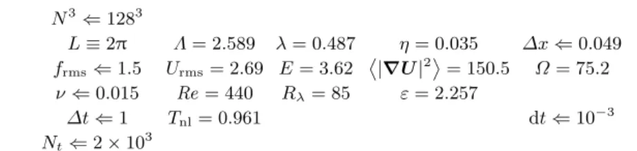
Figure 2. Two-dimensional horizontal cuts in the plane z = π/2 of the instantaneous total vertical velocity Uz(x, y, π/2) and total vertical vorticiy (∇ × U )z(x, y, π/2) at a single
time t = 2 × 10³
, represented in false colors from black (negative) to white (positive) with grey being around zero. Note the intense localised vortical structures present in the flow showing that the turbulence is already well developed, and that the symmetries of the forcing have been lost for the total flow at that Reynolds number. Also, these fields would both be identically zero for the forcing or the initial conditions.
by keeping the forcing amplitude constant at frms = 1.5 (so that the velocity Urms stay
at O(1)) and decreasing the viscosity ν, increasing the resolution N at the same time, so that the flow small scale structures are correctly resolved kmaxη > 1. Table 1 lists
all numerical parameters and measured global quantities for the numerical run that has been analysed in this paper.
We cannot however use very high Reynolds numbers, not only because we are limited by memory and computation time, but also because we want to run the simulation for very long times, thousands of eddy turnover times Tnl, to be able to compute the
mean flow by time averaging. Also, because we want to study homogeneity by studying indepently different locations and more specifically different planes in the z-direction, we will refrain from averaging statistical quantities over the whole simulation volume, meaning that the statistical noise could be large if this effect is not compensated by time averaging. Specifically, starting from the TG initial condition, we will integrate the flow for 103
∆t ≈ 103
Tnl eddy turnover time so that the turbulence has time to be
fully developed and the flow is statistically stationary. Then, we integrate the flow again for Nt∆t ≡ 2 × 10³∆t, saving a snapshot of the flow at every ∆t, that are essentially
uncorrelatated since ∆t & Tnl. These 2 × 10³ samples are then divided in two sets of
103
fields, that are analysed independently and then compared, so that we can have an idea of the remaining statistical fluctuations for 103
samples, and can ensure that this number of samples of the velocity field is enough to compute time and space averages.
We thus used a moderate resolution of N3
= 1283
, which may not seem very large, but allowed us to reach Reynold numbers Re around 450, enough to obtain a turbulent flow with velocity fluctuations having an energy of more than twice the mean flow as we will see in section 5. Figure 2 shows that the instantaneous velocity and vorticity closely reseembles a turbulent flow, and that the mean flow or the forcing are not apparent in these instaneous snapshots. Also, even if we will see in the next section that the mean flow has the symmetries of the TG forcing, the instantaneous velocity and the fluctuations have completely lost these symmetries. Of course, as the flow is spatially well-resolved numerically, the inertial range of turbulence won’t be very extended. Still, we will see
that energy transfer laws can be observed already at this resolution, provided we take into account the corrections due to the finite viscosity. Note that at this resolution, one snapshot of the three components of the velocity field in double precision is roughly 50 MBytes, so that we have in total about 100 GBytes of data to analyse, both for the total velocity and for its fluctuations.
4. Statistical averages and the mean-flow
It is well-known that, in contrast to for instance wind tunnel flows, the von K´arm´an swirling flow has a non-trivial tridimensional mean spatial structure that can be evidenced by long time exposure of flow tracers or by time averaging (see e.g. Ravelet, Chiffaudel & Daviaud (2008) or Monchaux, Ravelet, Dubrulle, Chiffaudel & Daviaud (2006)). Similarly, even at high Reynolds numbers, the Taylor-Green vortex has a mean flow that can be revealed by time averaging. Here, we will define precisely the averaging procedures that we will use to separate the mean flow and the fluctuations in the TG vortex, and to study homogeneity along the z-direction.
4.1. Time averages
Let us consider a vector or scalar quantity a(. . . ; x, y, z) defined in our turbulent flow. Then the time average will be simply given as expected by
a(. . . ; x, y, z) ≡ 1 T Z dt a(. . . ; x, y, z, t) (4.1) = 1 Nt Nt X l=0 a(. . . ; x, y, z, l∆t) , (4.2) where we recall that the time separation ∆t is such that the samples are effectively uncorrelated. In particular, we can separate the total flow U (x, y, z, t) into its different constituents, a static mean flow U (x, y, z) and turbulent fluctuations u(x, y, z, t) with
U(x, y, z, t) ≡ U (x, y, z) + u(x, y, z, t) (4.3) (U, V, W )T(x, y, z, t) ≡ ( U , V , W )T(x, y, z) + (u, v, w)T(x, y, z, t) . (4.4) We will now use capital letters to refer to the total turbulent flow U and lower case letters to refer to the turbulent fluctuations u, the different components being denoted by (U, V, W ) or (u, v, w). Note that by definition u (x, y, z) = 0. The mean flow U obtained by averaging over 2 × 10³
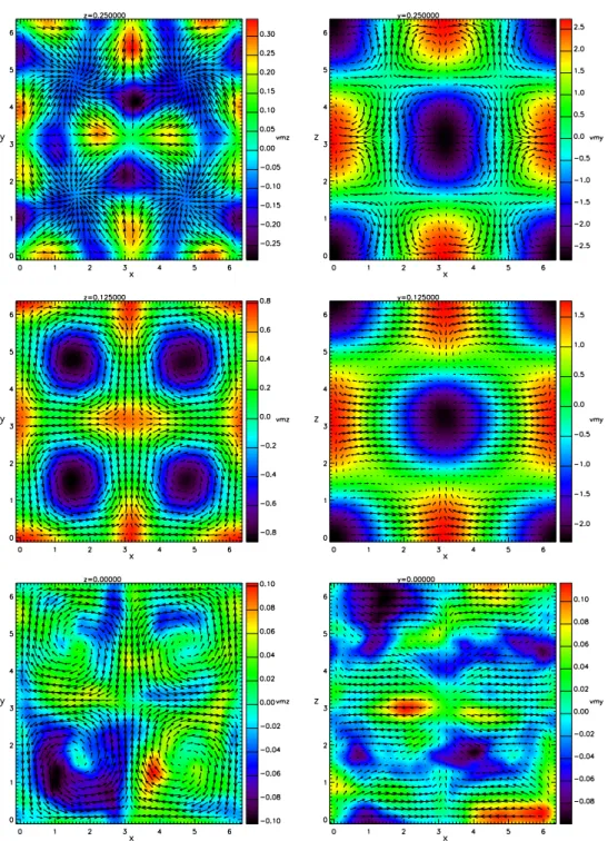
snapshots is shown in figure 3, as two-dimensional cuts along two directions, and at three different heights in the numerical volume. We emphasize that this mean flow U is not a solution of the Navier-Stokes equations when the flow has turbulent fluctuations u, as already stressed by (Monchaux, Ravelet, Dubrulle, Chiffaudel & Daviaud 2006). Still, we can see that even if the mean flow has developed specific features of its own, it has strong similarities with the forcing ; in particular, the symmetries of the forcing have been restored, and the mean flow consists of eight antisymmetrically replicated identical cells, with negligible differences that could be eliminated by increasing the averaging in time. The mean flow in the top, center or bottom planes z = kπ closely resembles the forcing and is dominated by the rotation with completely negligible vertical velocities (figure 3 bottom left, and top and center right). Due to the strong differential shear along the z-direction, the mean flow in the ‘halfway’ planes z = π/4 + kπ/2 has developed a large poloidal component (see figure 3 center left and right) that is superposed on the mean rotation, and reproduces the two recirculating cells observed in the experimental von K´arm´an flow (see figure 1 of Monchaux, Ravelet,
Figure 3. On the left, in-plane mean velocity horizontal components ( U , V ) (shown as arrows) and mean vertical velocity component W (shown as colors), shown for three horizontal planes z = π/2, z = π/4 and z = 0 (from top to bottom). On the right, in-plane mean velocity horizontal components ( U , V ) (shown as arrows) and mean vertical velocity component W (shown as colors), shown for three vertical planes y = π/2, y = π/4 and y = 0 (from top to bottom). In all of these figures, there is a 4-fold plane symmetry of the mean flow induced by the TG forcing.
Dubrulle, Chiffaudel & Daviaud (2006) or figure 1a of Huck, Machicoane & Volk (2017)). In the ‘middle’ planes z = π/2 + kπ where the forcing is zero, the flow has developed a non-trivial structure around a central stagnation point in the horizontal plane with two contracting directions x and y and one diverging z-direction (see figure 3 top left and right). This configuration has similarities, but does not reproduce the state observed by (Huck, Machicoane & Volk 2017) (see in particular their figure 3) who studied in detail the mean flow near the stagnation point at the middle of the von K´arm´an cell and found one of the horizontal directions diverging and the other converging, and exchanging their role in a slow random fashion. However, they used a square section vessel, and this seems to be the cause of this difference with the circular section cell, because the horizontal diverging and contracting directions are aligned with the walls of the cell. In our case, we also don’t have a circular symmetry, but a square symmetry. However, the use of periodic boundary conditions means that the large scale topology is different and one can see that the middle stagnation point has a horizontal converging circular symmetry, but there are also horizontally diverging points at the four ‘corners’ of the plane. These points would not exist in a circular or square cell with walls and show that the local topology of the mean flow can be induced by the boundaries, even from far away. The extent of the interactions between mean flow and turbulent fluctuations is however not clear. In particular, we find like (Huck, Machicoane & Volk 2017) that the turbulent fluctuations are maximal near the middle stagnation point, especially for the vertical z-directions, as we will develop in section 5.
4.2. Space averages
As we noted in section 2, statistical conservation laws like Kolmogorov, Yaglom or Monin’s law are derived under the assumption of homogeneity, i.e. we have to average over temporal and spatial scales large enough that the mean statistical properties of two-point quantities like structure functions or correlations become nearly independent of the center position of the two points (i.e. it becomes translationally invariant), and depends only on the separation between the two points. It is in fact not exactly clear how large this scale must be for turbulence, but the flow integral scale Λ is a good candidate and, for turbulence in a periodic box, the (larger) size of the box L is even better to reduce the statistical noise. So, we will define (global) space averages to be over the total volume of the box as
e a(. . . ; t) ≡ 1 L3 Z dz Z dy Z dx a(. . . ; x, y, z, t) (4.5) = 1 N3 N X i=0 N X j=0 N X k=0 a(. . . ; i∆x, j∆x, k∆x, t) . (4.6) For homogeneous isotropic turbulence (HIT), this spatial averaging would (by defi-nition) be unnecessary, as all statistical properties are assumed to be independent of position, and only further time averages are needed for statistical convergence. As our goal is precisely to study homogeneity in the TG vortex, especially as function of the z coordinate along the z axis, we will also use averages limited to horizontal planes at a given height z, but average over the x and y coordinates to reduce the statistical noise
b a(. . . ; z, t) ≡ 1 L2 Z dy Z dx a(. . . ; x, y, z, t) (4.7) = 1 N2 N X i=0 N X j=0 a(. . . ; i∆x, j∆x, z, t) . (4.8)
With these spatial averages definitions, we will compute global space-time averages by combining (4.1) and (4.5) or (4.7)
hai (. . .) ≡ ea (4.9)
or
hai (. . . ; z) ≡ ba , (4.10)
where we will be slightly abusing notation and using h. . .i for means over the whole vol-ume, or only a z-plane, the difference being apparent by the z dependence in the notation. When averages are limited to a given z-plane, and we are considering increments rzalong
the z direction, we have to be careful and center the increment around the z-plane of interest, that is use for instance U (x, y, z + rz/2, t) − U (x, y, z − rz/2, t) when computing
structure functions at height z.
As we already said, structure functions will be evaluated completely in physical space. This is a time-expensive computation, even for moderate resolutions like we have here. Indeed, for a single structure function, we have to average over N3
points in space, times Nt snapshots in time, times N increment separations, times 3 directions, that is
about 900 × 109
increment values to average and at least that number of flops and of memory accesses, for each computed structure function. For second-order ordrer structure functions, Discrete Fourier Transforms (FFTs) could be used to compute them from correlation functions, but we did not implement this method as it cannot be generalised to higher order structure functions.
5. Second-order statistical results
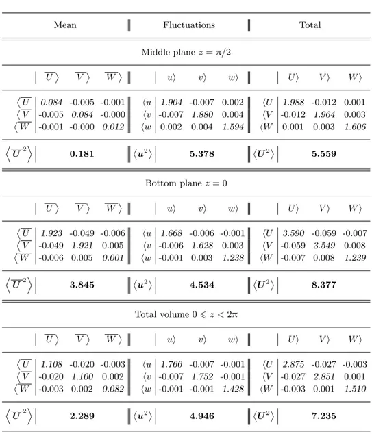
From the decompositions (4.3) and (4.4), we can compute the single point second order statistics for the total flow, the mean flow or the turbulent fluctuations, either in the whole volume, or in specific planes only. Results are presented in table 2 for all constituents of the flow in all directions, either in the whole volume, or in the bottom plane z = 0 where rotation is maximal, or in the ‘middle’ plane z = π/2 where both rotation and mean flow are small (see figure 3). Several comments are in order.
First, we can note the absence of cross correlations between different velocity compo-nents, for all constituents of the flow we find thatUi Uj®(z), huiuji (z) and hUiUji (z)
are close to zero for i 6= j and for all z. For the mean flow, this property comes from the pure shear form of the forcing that satisfies
hfifji (z) = 4 f 2 rms cos2 (z) 4 δij(1 − δi3) , (5.1)
i.e. its is purely diagonal (but not isotropic hfzfzi (z) = 0) for all heights z with a
non-homogeneous total variance f2®(z) that changes with z (2 f2
rms for z = 0, f 2 rms
for z = π/4 and 0 for z = π/2) and that is equal to f2
rms for the whole volume. For the
fluctuations and the total flow, this absence of cross-correlations would be an indication of isotropic turbulence as indeed the two horizontal variances are always nearly equal, but the vertical component variance is significantly smaller than the two horizontal ones by a factor of nearly 2 for the total flow in the whole volume. This is not surprising for the total flow in the top or bottom plane where the mean flow is dominant, but remains true even for the velocity fluctuations in the middle plane z = π/2 where the vertical variance is 15 % smaller than the two horizontal ones. In the whole volume, the fluctuations vertical variance is smaller by 20 % than the the horizontal ones, so the turbulent velocity fluctuations are more isotropic than the total flow, but not completely so.
Mean Fluctuations Total Middle plane z = π/2 U¸ V¸ W¸ ui vi wi U i V i W i ˙ U 0.084 -0.005 -0.001 hu 1.904 -0.007 0.002 hU 1.988 -0.012 0.001 ˙ V -0.005 0.084 -0.000 hv -0.007 1.880 0.004 hV -0.012 1.964 0.003 ˙ W -0.001 -0.000 0.012 hw 0.002 0.004 1.594 hW 0.001 0.003 1.606 D U2E 0.181 ˙u2¸ 5.378 ˙U2¸ 5.559 Bottom plane z = 0 U¸ V¸ W¸ ui vi wi U i V i W i ˙ U 1.923 -0.049 -0.006 hu 1.668 -0.006 -0.001 hU 3.590 -0.059 -0.007 ˙ V -0.049 1.921 0.005 hv -0.006 1.628 0.003 hV -0.059 3.549 0.008 ˙ W -0.006 0.005 0.001 hw -0.001 0.003 1.238 hW -0.007 0.008 1.239 D U2E 3.845 ˙u2¸ 4.534 ˙U2¸ 8.377 Total volume 0 6 z < 2π U¸ V¸ W¸ ui vi wi U i V i W i ˙ U 1.108 -0.020 -0.003 hu 1.766 -0.007 -0.001 hU 2.875 -0.027 -0.003 ˙ V -0.020 1.100 0.002 hv -0.007 1.752 -0.001 hV -0.027 2.851 0.001 ˙ W -0.003 0.002 0.082 hw -0.001 -0.001 1.428 hW -0.003 0.001 1.510 D U2E 2.289 ˙u2¸ 4.946 ˙U2¸ 7.235
Table 2. Covariance matrices of the velocity components and total variance for the mean velocity ˙ Ui Uj¸, the velocity fluctuations huiuji and the total velocity hUiUji, for two
horizontal planes at z = 0 and z = π/2 and for the total TG vortex volume 0 6 z < 2π.
The velocity fluctuations energy accounts for ≈ 70 % of the total flow energy for the whole volume, but only for ≈ 55 % in the top or bottom plane, while it is completely dominant in the middle planes where it accounts for 97 % of the total energy (fluctuations energy is ≈ 30 times larger than the mean flow in the middle plane). In fact, while the mean flow energy decreases by a factor of ≈ 20 between the bottom and middle planes, the fluctuations variance increases only by 17 % with respect to its global volume mean, so that the total energy changes by 40 % with respect to this global mean. The turbulent fluctuations are thus more homogeneous than the total flow, but still vary
10−1 100 Separation, ri 10−2 10−1 100 101 Structure function, Sij (ri ) UU,z=0 UU,z=π/2 WW,z=0 WW,z=π/2 10−1 100 Separation, ri 10−2 10−1 100 101 Structure function, Sij (ri ) uu,z=0 uu,z=π/2 ww,z=0 ww,z=π/2
Figure 4. Second-order longitudinal structure functions ˙[∆Ui(ri)] 2
¸for the horizontal U component of the velocity (circles) and the vertical W component (squares) in two horizontal planes at z = 0 (empty symbols) and z = π/2 (filled symbols) for the total velocity U (left) and the turbulent fluctuations u (right). The long dashed line is an r2
law showing that the structure functions are quadratic at small scales and that the simulation is indeed well-resolved.
significantly as a function of the height, and measuring accurately the total energy of the flow requires measurements in the whole volume. Also, we emphasize that these deviations from homogeneity are measured by averaging over whole planes in the flow, and it is highly probable that even larger deviations could be measured by restricting the averaging domain around specific locations, like the center point of the middle planes, as was indeed observed by (Huck, Machicoane & Volk 2017).
An observation that can be made from table 2 is that the fluctuations energy is not independent of the mean flow energy, but it is anticorrelated , the fluctuations being larger where the mean flow is weaker. This is true even if the mean flow and the turbulent fluctuations are uncorrelated, either globally or in specific planes, i.e.
hUiUji (z) =Ui Uj®(z) + huiuji (z) , (5.2)
so that this link between their magnitudes DU2E andu2®
in different planes is not a priori obvious.
5.1. Second-order homogeneity
We now turn to the subject of the homogeneity of two points second order statistics by looking at second order longitudinal structure functions in different planes z, either for the total velocity U or its turbulent fluctuations u. Examples are shown in figure 4 for U on the left and for u on the right, for the x and z velocity components and at two different heights z = 0 and z = π/2. One can first notice that no inertial range scaling is observed in the structure functions, which is not surprising since the Reynolds number is not very large, and observing a clear inertial range is much more difficult for structure functions than for spectra, the latter switching from a power law to an exponential behaviour at small scales, while the former switches between two power laws. On the other hand, a clear quadratic behaviour is shown at small scales, showing that the velocity field is regular and that small spatial scales are correctly resolved.
One can see from the graphs that, even if the second order statistics are quite different at large scales for different components or different planes, they come closer together as we move towards smaller scales. Still, even at the smallest scale reached in the simulation ∆x, there are significant differences of nearly 20 % between structure functions measured at z = 0 and z = π/2 for the total velocity. Interestingly, these differences are even stronger for the turbulent fluctuations, reaching up to ≈ 30 %
10−2 10−1 100 Longitudinal structure function, Sii(ri)
10−1 100 101
Transverse structure function,
Sii (rj ) UW,z=0 UW,z=π/2 WU,z=0 WU,z=π/2
Figure 5.Transverse structure functions˙[∆Ui(rj)] 2
¸ plotted as a function of the corresponding longitudinal structure functions˙[∆Ui(ri)]
2
¸ for i ≡ x, j ≡ z (circles) and i ≡ z, j ≡ x (squares) in two horizontal planes at z = 0 (empty symbols) and z = π/2 (filled symbols). The long dashed line corresponds to the ratio 2 that is expected for isotropic turbulence regular (smooth) at small scales.
between the two planes. These differences are much larger than those between different components in the same plane, showing that small scale inhomogeneities are important in the TG flow, so that measurements of the local small-scale energyD[∆Ui(ri)]
2E
or of the local dissipation 15 ν limr→0
D
[∆Ui(ri)] 2E
/r2
using isotropy will give different results if measured at different heights z.
5.2. Second-order isotropy
Local and global isotropy are key ingredients to obtain Yaglom’s law (1.4) and Kol-mogorov’s law (1.1) respectively, so it is important to verify if they come realised in the TG flow at small scales. Local isotropy simply means that all directions are locally equivalent for the turbulent velocity field, at least at small scales. While that property is not evident if the turbulence forcing is anisotropic as it is for the TG forcing (3.1), it is generally believed to be true, or postulated, for fluid turbulence. Figure 4 show that it is indeed reasonably verified in the TG turbulent flow, with the horizontalD[∆Ux(rx)]
2E
and the vertical D[∆Uz(rz)] 2E
being undistinguishable at small scales r in the two planes z = 0 and z = π/2 (but differ between the two planes as noted in the previous section), even though their large scale variances Ux
2
and Uz 2
differ significantly (see table 2). Local small scale isotropy thus seems a tenable option for the TG vortex flow. Global isotropy is a deeper property that links the velocity statistics in different orthogonal directions using isotropy and incompressibility. For second-order statistics, it implies for instance (see Monin & Yaglom (1975) or Hinze (1959))
D [∆Uj(ri)] 2E =D[∆Ui(ri)] 2E +r 2 ∂D[∆Ui(ri)] 2E ∂r j 6= i , (5.3)
10−1 100 Separation, ri 0 1 2 3 Transverse/Longitudinal, Sii (rj )/S ii (ri ) UW,z=0 UW,z=π/2 WU,z=0 WU,z=π/2 10−1 100 Separation, ri 0 1 2 3 Transverse/Longitudinal, Sii (rj )/S ii (ri ) uw,z=0 uw,z=π/2 wu,z=0 wu,z=π/2
Figure 6. Ratio between second-order transverse ˙[∆Ui(rj)] 2¸
and longitudinal structure functions ˙[∆Ui(ri)]
2
¸ for i ≡ x, j ≡ z (circles) and i ≡ z, j ≡ x (squares) in two horizontal planes at z = 0 (empty symbols) and z = π/2 (filled symbols) for the total velocity U (left) and the turbulent fluctuations u (right).
that links the transverseD[∆Uj(ri)] 2E
and longitudinalD[∆Ui(ri)] 2E
structure functions. In particular, if the longitudinal structure function is a power law with exponent ζ2, the
transverse one will also be a power law with the same exponent and an amplitude that differs by a factor 1 + ζ2/2 (see e.g. Noullez, Wallace, Lempert, Miles & Frisch (1997)
for experimental measurements of transverse structure functions), so that if at small scales the flow becomes regular with a quadratic behaviour of the second-order structure functions, the transverse and longitudinal ones should differ by a factor of 2, a fact used in equ. (2.14).
Figure 5 plotting the transverse structure function as a function of the longitudinal one for the total velocity shows however that this relation is not very well statisfied, with discrepancies of more than 20 % from the factor 2 (materialised by the long dashed line) at the small scales. For instance, the transverse D[∆Ux(rz)]
2E
is about 2.5 times the longitudinal D[∆Ux(rx)]
2E
in the middle plane z = π/2, showing once again the strong anisotropy of that zone (Huck, Machicoane & Volk 2017). This discrepancy is also visualised in figure 6, where the ratio between transverse and longitudinal structure functions is plotted as a function of scale, and shows that this ratio does not go to 2, neither for the total flow (left) or the turbulent fluctuations (right). These same ratios computed for the full TG simulation volume display exactly the same behaviour, and show that global isotropy is not fully satisfied in the TG flow with forcing, with significant departures from relations (2.14). Whether these discrepancies will decrease and eventually disappear when the Reynolds number increases is an open question, but at least it means that using relations like (2.15) should be done with caution in flows with anisotropic mean flow or forcing.
6. Energy transfer and dissipation
We will now study third-order structure functions, either the standard longitudinal ones or the mixed third-order structure function (2.8) defining the energy flux vector, in the context of the validation of the Kolmogorov, Yaglom or Monin’s energy transfer laws. We stress that these odd-order structure functions are computed without using any absolute values in their definition, as we will compare their value with those coming from the corresponding law, i.e. (1.3), (2.11) and (2.7), without any adjustable parameter,
10−1 100 Separation, rx 10−1 100 Integrated dissipation −〈(∆Ux) 3 〉 6ν ∂x 〈(∆Ux) 2 〉 Totalx 4/5 εrx 10−1 100 Separation, rz 10−1 100 Integrated dissipation −〈(∆Uz) 3 〉 6ν ∂z 〈(∆Uz) 2 〉 Totalz 4/5 εrz
Figure 7. The two terms of the l.h.s. of the Kolmogorov equation (1.1), turbulent transfer (circles) and viscous dissipation (squares), and their sum (lozenges) as a function of scale, compared to the Kolmogorov prediction 4/5 ε r shown as a long dashed line. The averages are computed for the total velocity U in the full volume, and correspond to increments in the horizontal x direction on the left, and in the vertical z direction on the right.
because the dissipation has been measured independently in the spectral DNS code as ε = ν |∇ × U |2®
. The resulting value of these structure functions thus involves a lot of cancellations between positive and negative values of the longitudinal velocity increment and only comes from the slight asymmetry of the distribution of ∆Ui(ri). Averaging over
a large number of nearly independent times is then required to ensure the convergence of these structure functions. While studying the energy transfer laws, we will also check the validity of the various computational definitions of the dissipation equ. (2.6), (2.12) and (2.15), as the total dissipation will be controlled only by the viscous dissipation at small scales.
Figure 7 shows the two terms of the l.h.s. of the finite Reynolds number Kolmogorov relation (1.1), as well as their sum, computed in the whole simulation volume for the total velocity U in the horizontal x direction on the left, and in the vertical z direction on the right. Both sums should be proportional to the total integrated dissipation from 0 to r and thus scale linearly according to the Kolmogorov prediction 4/5 ε r. A first point to note is that, at this small Reynolds number, no inertial range can be observed in the third-order longitudinal structure functions themselves (circles), so the transfer term alone D[∆ui(ri)]
3E
has no linear behaviour (it rather displays a cubic behaviour at small scales, implying that the flow is regular and that the numerical simulation is well resolved) and Kolmogorov’s ‘law’ (1.3) is not verified. This is to be expected, as previous computations of (Gotoh, Fukayama & Nakano 2002) and (Mininni, Alexakis & Pouquet 2008) showed that the approach to pure scaling laws is very slow and that very large Reynolds numbers would be needed to observe (1.3) without viscous correction. Our goal here is rather to check whether the complete law (1.1) and isotropy holds for the TG flow. The viscous terms (squares) differ only by ≈ 10 % between the horizontal and vertical directions at small scales and are close to the Kolmogorov value, so that using second-order structure functions to estimate the dissipation using (2.15) is reasonable, provided the small scales are correctly resolved (either numerically in the TG flow or experimentally in the von K´arm´an flow). On the other hand, using the transfer term alone never gives a reliable estimation of ε unless the Reynolds numbers is very large, an effect already noted by various authors (see e.g. fig. 2 of Antonia, Ould-Rouis, Anselmet & Zhu (1997) or fig. 12 of Gotoh, Fukayama & Nakano (2002)). Using the sum of the viscous and transfer terms (if they can be measured reliably) gives a result that is not too far away from the Kolmogorov linear scaling, but there are significant differences between the
10−1 100 Separation, rx 10−1 100 Integrated dissipation −〈|∆U|2 ∆Ux 〉 2ν ∂x 〈|∆U| 2 〉 Totalx 4/3 εrx 10−1 100 Separation, rz 10−1 100 Integrated dissipation −〈|∆U|2 ∆Uz 〉 2ν ∂z 〈|∆U| 2 〉 Totalz 4/3 εrz
Figure 8.The two terms of the l.h.s. of the Yaglom equation (1.4), turbulent transfer (circles) and viscous dissipation (squares), and their sum (lozenges) as a function of scale, compared to the Yaglom prediction 4/3 ε r shown as a long dashed line. The averages are computed for the total velocity U in the full volume, and correspond to increments in the horizontal x direction on the left, and in the vertical z direction on the right.
10−1 100 Separation, rx 10−1 100 Total dissipation − ∂x 〈|∆U| 2 ∆Ux 〉 2ν ∂x 2 〈|∆U|2〉 Totalx 4/3 ε 10−1 100 Separation, rz 10−1 100 Total dissipation − ∂z 〈|∆U| 2 ∆Uz 〉 2ν ∂z 2 〈|∆U|2 〉 Totalz 4/3 ε
Figure 9. Computed derivatives of all terms of the Yaglom relation (1.4), as a function of scale r, as well as the Yaglom prediction of the constant slope 4/3 ε. All symbols and conditions as in figure 8.
horizontal and vertical directions for the TG flow, due mostly to the horizontal transfer term overestimating the total dissipation at intermediate scales, while the vertical one underestimates it. This could be due the smaller variance of the velocity in the vertical direction, or to the rotational part of the mean flow that cannot be completely neglected in the total flow, and that could partly inhibit energy transfers in the vertical direction. Arguments if favor of one or these possible explanations can be obtained by looking at the Yaglom and Monin laws.
Figure 8 is exactly similar to figure 7, but this time shows the different terms in the Yaglom relation, whose sum should scale linearly like 4/3 ε r. Once again, no inertial range is present in the mixed third-order structure function (circles) due to the limited Reynolds number, but the sum of the transfer and viscous terms is very close to the linear Yaglom prediction. Also, the horizontal (left) and vertical (right) directions appear nearly identical. To check that this really the case, it is better to look at the derivatives (computed here using 3 points finite differences) of the different terms, that are shown in figure 9. One can then see that, even if the x and z directions are very similar, and that the sums of the derivatives are close to the Yaglom prediction 4/3 ε, they have slight differences. In particular, the transfer in the x direction (and thus the total dissipation) starts from a lower value than the transfer along z, but increases faster with scale so that the apparent total dissipation along x increases with scale, while it decreases for z (the same effect is observed for the Kolmogorov law). For the Yaglom relation, the transfer
10−1 100 Separation, r 100 101 Total dissipation − ∇⋅ 〈|∆U|2∆U〉 2ν ∇2〈|∆U|2 〉 Total 4 ε
Figure 10. The two terms of the l.h.s. of Monin’s equation (1.5), turbulent transfer (circles) and viscous dissipation (squares), and their sum (lozenges) as a function of scale, compared to the constant prediction 4 ε shown as a long dashed line. Averages are computed for the total velocity U in the full volume.
term corresponds to the dissipation of the total energy |∆U (ri)|2 by the longitudinal
velocity fluctuations ∆Ui(ri), so we can make the hypothesis that this reduction of the
transport is due to the lower amplitude of the velocities in the vertical direction when we go to larger scale, and the flow is more rotational. At small scales, the velocity gradients along z are slightly larger by about 15 % than the gradients along x, probably due to the fact that the total velocity z component is mostly due to the turbulent fluctuations that act at small scales, while the total velocity x component also has large scale constituents coming partly from the mean flow. Measuring the dissipation through (2.12) will thus not always be completely reliable if the flow has anisotropic inhomogenities like the TG flow has. Also, it must be noted that, even if small, the transfer term does not vanish immediately when going to small scales, and gives a finite contribution to the total dissipation at nonzero scales, that only goes to zero like r2
when the flow is regularised by the viscosity.
The fact that the Yaglom relations along x and z have opposite deviations from a linear behaviour suggests that some ‘average’ between them might give a perfectly linear relationship, and this in fact what Monin’s relation will produce. Figure 10 shows the two terms on the l.h.s. of Monin’s relation (with derivatives computed again using 3-points finite differences), and shows that their sum manages to stay constant for about one decade of scales even at this low resolution, and has the correct value 4 ε to better than 2 %. Several comments are in order. It might come as a surprise that Monin’s relation is already valid at such a low Reynolds number, but its derivation does not require the assumption of zero viscosity if we include the viscous dissipation term. Homogeneity is needed, but is clearly satisfied in our case if we average over the full volume of a 2π-periodic box and the forcing also has these symmetries. Interestingly, the transfer term alone goes to a maximum that nearly coincides with the right value for the total dissipation (the error is only 3 %), but it does so at only one scale, while the sum of the viscous and dissipative terms stays constant from the smallest scale to the scale of maximum transfer (note that the viscous term 2 ν ∇2
|∆u(r)|2®
10−1 100 Separation, r 10−1 100 101 Integrated dissipation −1r⋅ 〈|∆U| 2 ∆U〉 2ν ∇⋅ 〈|∆U|2〉 Total 4 εr
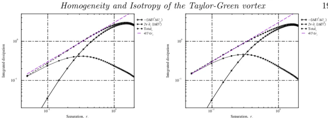
Figure 11.‘Isotropically integrated’ terms of Monin’s equation (1.5), corresponding to the sum of Yaglom’s equation (1.4) in the three directions r, compared to the prediction 4 ε r. Conditions and symbols as in figure 10.
intermediate scales r ≈ 0.32). The total dissipation apparently goes to zero at large scales, but this is because we did not compute the work of the forcing that has to act at these scales to maintain a steady state. Also, it is only because we averaged over very long times that we could observe Monin’s law with stationary values of all terms, because all the terms in the complete Monin’s relation (2.4) are fluctuating in time with varying characteristic times at each scale. Because Monin’s relation is a form of ‘weighted sum’ of the derivatives of Yaglom’s law in the different directions, we can also compute a ‘sum’ of Yaglom’s laws as an ‘isotropically integrated’ Monin’s law
−X i D |∆U (r 1i)| 2 ∆Ui(r 1i) E + 2 ν X i ∂i D |∆U (r 1i)| 2E = 4 ε r , (6.1) summing the mixed third-order structure functions and the total second-order structure functions at the same separation in the three different directions. This ‘integrated’ form of Monin’s relation that should be valid also for anisotropic homogeneous flows is shown in figure 11 and we can see that it is well-verified in the TG flow even at low Reyynolds numbers. One can notice that the viscous and transfer terms become equal and cross each other at a scale that has to be related to the Kolmogorov scale η, but differs between Monin’s relation where it is ≈ 4 η, and its integrated form where it is around 8 η. Still, this means that one or both forms of Monin’s law can be used to observe η only from experimental measurements of the velocity U , if the fluid viscosity ν is known.
As we said in the the intoduction, turbulent fluctuations with respect to the mean flow due to forcing are often believed to be closer to homogeneous isotropic turbulence than the total flow. They are indeed slightly more isotropic, as we showed in section 5, but they are farther when we consider exact energy transfer laws, as figure 12 demonstrates. One can see that all terms of Monin’s relation (1.5) computed for the velocity fluctuations u, and also their sum, have values that are much lower than the expected total dissipation 4 ε. This could be attributed to the amplitude of the fluctuations being smaller than those of the total velocity that is used to compute ε, and indeed one can see that the dissipative term alone is too small and does not reach the correct value of the total dissipation at
10−1 100 Separation, r 100 101 Total dissipation − ∇⋅ 〈|∆u|2∆u〉 2ν ∇2〈|∆u|2 〉 Total 4 ε
Figure 12.The same quantities and conditions as in figure 10, but computed for the velocity fluctuations u instead of the total velocity U .
10−1 100 Separation, r 100 101 Total dissipation − ∇⋅ 〈|∆U|2 ∆U〉 2ν ∇2 〈|∆U|2〉 Total 4 ε 10−1 100 Separation, r 100 101 Total dissipation − ∇⋅ 〈|∆U|2 ∆U〉 2ν ∇2 〈|∆U|2〉 Total 4 ε
Figure 13.The same quantities and conditions as in figure 10, computed for the total velocity U , but averaging only in the plane z = 0 (left) and only in the plane z = π/2 (right).
small scales. But the transfer term is also too small and does not go at all to the total dissipation, so that the sum of the two terms does not show any constant plateau as a function of scales. This implies that the distribution of total dissipation across scales for the turbulent fluctuations, and its decomposition in transfer and viscous terms, do not correspond to those of a turbulent velocity field. This could have been expected as the turbulent fluctuations u are not solutions of the Navier-Stokes equations (nor does the mean velocity field U ) and so have no reason to obey (1.5).
A final comment about Monin’s law (and of course to an even greater extent for Yaglom an Kolomogorov law) is that it is realised only if averaging over scales such that the flow has become homogeneous. Otherwise, quantities like the mean dissipation are not even well-defined. For example, figure 13 displays the different terms of Monin’s relation computed for the total velocity U in the same conditions as in figure 10, but averaging only in the planes z = 0 (left) and z = π/2 (right). One can see that the sum of the terms, that is the total dissipation, is slightly too low at small scales in the bottom plane, mainly due to a lack of dissipation, and slightly too high at large scales, due to an excess of transfer, so that the total dissipation increases with scale. Opposite deviations (excess of dissipation and lack of transfer) occur in the middle plane z = π/2. One should note
that, because Monin’s law computes an average between the three directions, it requires increments also along the z direction that, as we said in section 4.2, are centered on the considered z position, but involve larger vertical separations as the scale increase. Still, it means that the TG flow has strong inhomogeneities that can affect the local energy dissipation rate (as was also observed experimentally by Huck, Machicoane & Volk (2017), and this effect can be evidenced using Monin’s energy transfer relation that is independent of isotropy, but requires homogeneity. This means that its violation implies either inhomogeneities, or that the velocity field does not obey Navier-Stokes equations, as we pointed out in the previous section.
7. Discussion and conclusions
We have checked the applicability of the Kolmogorov, Yaglom and Monin energy transfer laws for a strongly anisotropic and inhomogeneous flow, namely the stationary TG vortex that develops from a large scale constant in time TG forcing 3.1. This large scale forcing induces an anisotropic non-homogenous mean flow that is not negligible with respect to the turbulent fluctuations and, more importantly, does not disappear when the Reynolds number becomes very large (Ravelet, Chiffaudel & Daviaud 2008). Although the velocity fluctuations have been found to be more isotropic and homogeneous than the total flow at the level of one and two points second-order statistics, they still show strong deviations from Homogeneous and Isotropic Turbulence, with statistcal properties that depend on position and orientation in the flow (see also Huck, Machicoane & Volk (2017)). These discrepancies can be observed in the finite Reynolds number Kolmogorov and Yaglom laws that show deviations from a linear behaviour and an apparent total integrated dissipation ε r that change with scale, location and direction. On the other hand, Monin’s law with the finite Reynolds number viscous correction remains valid in these non-ideal flows and provides a reliable way to estimate the total mean dissipation ε in the flow, even if its measurement in experimental conditions has practical difficulties (but see Lamriben, Cortet & Moisy (2011)). Monin’s law can be seen an ‘isotropic mean’ of Yaglom’s law in all space directions (see (6.1) and figure 11) and, as such, it might not be surprising that it remains valid as it is averaged in orientation (because of the sums in the divergence and laplacian) and position (because of the assumption of homogeneity). Still, it is reassuring that it is valid in the TG flow provided we average over a volume sufficient for the flow to be considered as homogeneous. Intriguingly, the derivation of Monin’s law does not use the hypothesis of turbulence of the flow, but only homogeneity, incompressibility and the fact that it satisfies the Navier-Stokes equation. It should thus also be valid at very low Reynolds numbers and for scales in the inertial range, provided we include in (2.4) the time derivative term if the flow is not stationary (for example in decaying turbulence) and/or the forcing term if we consider such large scales that the work of the forcing is not negligible. In fact, we plan in future work to check Monin’s relation in decaying turbulence or in static flows.
On the other hand, Monin’s relation (as well as Kolmogorov or Yaglom laws) requires homogeneity and we have demonstrated that it is not verified if we restrict its averaging region to inhomogeneous regions of the flow. Also, the velocity fluctuations with respect to the mean flow do not by themselves obey the Navier-Stokes equations and so do not statisfy Monin’s equation ; even if they contribute a significant part of the total dissipation, part of the total dissipation is missing in the fluctuations. In fact, some part of the dissipation is contained in the mean flow, even if it is also not a solution of Navier-Stokes equations. Figure 14 demonstrates this fact by computing the different terms of Monin’s relation for the mean flow U and shows that, even if the small scale viscous