HAL Id: hal-00317258
https://hal.archives-ouvertes.fr/hal-00317258
Submitted on 19 Mar 2004
HAL is a multi-disciplinary open access
archive for the deposit and dissemination of
sci-entific research documents, whether they are
pub-lished or not. The documents may come from
teaching and research institutions in France or
abroad, or from public or private research centers.
L’archive ouverte pluridisciplinaire HAL, est
destinée au dépôt et à la diffusion de documents
scientifiques de niveau recherche, publiés ou non,
émanant des établissements d’enseignement et de
recherche français ou étrangers, des laboratoires
publics ou privés.
High- and mid-latitude quasi-2-day waves observed
simultaneouslyby four meteor radars during summer
2000
E. Merzlyakov, D. Pancheva, N. Mitchell, J. M. Forbes, Yu. I. Portnyagin, S.
Palo, N. Makarov, H. G. Muller
To cite this version:
E. Merzlyakov, D. Pancheva, N. Mitchell, J. M. Forbes, Yu. I. Portnyagin, et al.. High- and
mid-latitude quasi-2-day waves observed simultaneouslyby four meteor radars during summer 2000.
An-nales Geophysicae, European Geosciences Union, 2004, 22 (3), pp.773-788. �hal-00317258�
SRef-ID: 1432-0576/ag/2004-22-773 © European Geosciences Union 2004
Annales
Geophysicae
High- and mid-latitude quasi-2-day waves observed simultaneously
by four meteor radars during summer 2000
E. Merzlyakov1, D. Pancheva2, N. Mitchell2, J. M. Forbes3, Yu. I. Portnyagin1, S. Palo3, N. Makarov1, and H. G. Muller4
1Institute for Experimental Meteorology, SPA Typhoon, Obninsk, Russia
2Department of Electronic & Electrical Engineering, The University of Bath, BA2 7AY, UK
3Department of Aerospace Engineering Sciences, University of Colorado, Boulder, CO 80309, USA
4Cranfield University, Royal Military College of Science, Shrivenham, UK
Received: 17 June 2003 – Revised: 7 July 2003 – Accepted: 1 September 2003 – Published: 19 March 2004
Abstract. Results from the analysis of MLT wind
mea-surements at Dixon (73.5◦N, 80◦E), Esrange (68◦N, 21◦E),
Castle Eaton (UK) (53◦N, 2◦W), and Obninsk (55◦N,
37◦E) during summer 2000 are presented in this paper.
Us-ing S-transform or wavelet analysis, quasi-two-day waves (QTDWs) are shown to appear simultaneously at high- and mid-latitudes and reveal themselves as several bursts of wave activity. At first this activity is preceded by a 51–53 h wave with S=3 observed mainly at mid-latitudes. After a short re-cess (or quiet time interval for about 10 days near day 205), we observe a regular sequence of three bursts, the strongest of them corresponding to a QTDW with a period of 47–48 h and S=4 at mid-altitudes.
We hypothesize that these three bursts may be the result of constructive and destructive interference between several spectral components: a 47–48 h component with S=4; a 60-h component with S=3; and a 80-h component with S=2. The magnitudes of the lower (higher) zonal wave-number com-ponents increase (decrease) with increasing latitude. The S-transform or wavelet analysis indicates when these spec-tral components create the wave activity bursts and gives a range of zonal wave numbers for observed bursts from about 4 to about 2 for mid- and high-latitudes. The main spec-tral component at Dixon and Esrange latitudes is the 60-h oscillation with S=3. The zonal wave numbers and frequen-cies of the observed spectral components hint at the possible occurrence of the nonlinear interaction between the primary QTDWs and other planetary waves. Using a simple 3-D non-linear numerical model, we attempt to simulate some of the observed features and to explain them as a consequence of the nonlinear interaction between the primary 47–48 h and the 9–10 day waves, and the resulting linear superposition of primary and secondary waves. In addition to the QTDW bursts, we also infer forcing of the 4-day wave with S=2 and the 6–7 day wave with S=1, possibly arising from nonlinear decoupling of the 60-h wave with S=3. The starting mecha-nism for this decoupling is the Rossby wave instability (e.g.
Correspondence to: E. Merzlyakov
(eugmer@typhoon.obninsk.org)
Baines, 1976). This result is consistent with the day-to-day wind variability during the observed QTDW events. An in-teresting feature of the final stage of the observed QTDW activity in summer 2000 is the occurrence of strong 4–5 day waves with S=3.
Key words. Meteorology and atmospheric dynamics
(mid-dle atmosphere dynamics; waves and tides; general or mis-cellaneous)
1 Introduction
There are not very many planetary-scale waves in the vicinity of the summer mesopause that have amplitudes of ∼tens m/s and are regularly observed from one year to another. First of all, there are diurnal and semidiurnal tides, and secondly, there are QTDWs (quasi-two-day waves). Herein, we con-sider QTDWs to include those oscillations with frequencies
between about 0.5±0.1 cycles day−1or periods of 40–60 h.
Since the early 1970s (Muller, 1972; Kal’chenko and Bul-gakov, 1973) these waves have been revealed in mesopause wind variations at low- and mid-latitudes. Glass et al. (1975) estimated the zonal wave number of this oscillation to be S=3. At present two main mechanisms have been proposed to explain the occurrence of the QTDW at levels of the meso-sphere/lower thermosphere (MLT). The first one considers these waves as a manifestation of the Rossby-gravity (3,0) normal mode forced by the lower atmosphere (Salby, 1981). The second mechanism considers the waves as a result of the instability above the summer stratospheric westward jet as was proposed by Plumb (1983) and extended to two-dimensions by Pfister (1985). Salby and Callaghan (2001) explored the relationship between the Rossby-gravity mode and the instability. Their analysis recovered major features of the QTDW, including twice-yearly amplification around solstice through interaction with easterlies. Their calcula-tions also revealed a wave number 4 component that exhibits less of the modal structure in comparison to wave number 3 component, and that should be more prevalent during July than during January.
774 E. Merzlyakov et al.: High- and mid-latitude quasi-2-day waves zonal wind, UK m/s -30 -20 -10 0 10 20 30 153 169 185 201 217 233 249 meridional wind, UK m/s -40 -30 -20 -10 0 10 20 30 40 153 169 185 201 217 233 249 zonal wind, Obninsk
m/s -30 -20 -10 0 10 20 30 153 169 185 201 217 233 249
meridional wind, Obninsk
m/s -40 -30 -20 -10 0 10 20 30 40 153 169 185 201 217 233 249 zonal wind, Esrange 90km
m/s -30 -20 -10 0 10 20 30 153 169 185 201 217 233 249
meridional wind, Esrange 90km
m/s -40 -30 -20 -10 0 10 20 30 40 153 169 185 201 217 233 249 zonal wind, Dixon
m/s -30 -20 -10 0 10 20 30 153 169 185 201 217 233 249 days from January 1
meridional wind, Dixon
m/s -40 -30 -20 -10 0 10 20 30 40 153 169 185 201 217 233 249 days from January 1
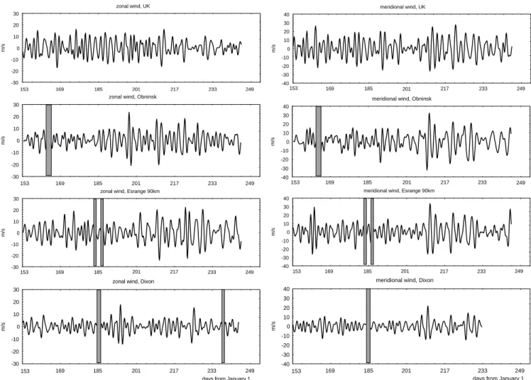
Fig. 1. (left) Zonal and (right) meridional components of the winds observed from day 153 (1 June) to day 244 (31 August) in 2000. Data
have been band-pass filtered to retain periods between 28 and 100 h. The longest gaps are shaded.
Analysis of wind data taken from several sites situated in a narrow latitudinal belt provides an opportunity to estimate the zonal wave number S of the investigated waves. Some recent results (Meek et al., 1996; Thayaparan et al., 1997; Jacobi et al., 2001) demonstrate that the range of this number is from 3 to 5 and more frequently, it is 3–4 for the Northern Hemisphere.
Numerical simulations using linear models (Hagan et al., 1993; Salby and Callaghan, 2001) and some global circula-tion models (Palo et al., 1999) suggest the QTDW with S=3 to be the Rossby-gravity mode. However, the waves with S=4–5 with slower phase speeds cannot as readily propagate from the lower to upper atmospheric levels and attain signif-icant amplitudes at MLT heights. Simulations with global circulation models by Norton and Thuburn (1996), and Mayr et al. (2001) demonstrate that strong QTDWs with large wave numbers (4–5) can be forced in situ by baroclinic instability in the presence of strong radiative and dissipative damping and full nonlinear dynamics.
The presence of the QTDW in the high-latitude MLT re-gion has been realized since the early investigations of the
wind circulation there (R¨uster et al., 1988; van Eyken et al., 2000). However, to date there have been no estimates of the zonal wave numbers for these waves at high latitudes. The waves have been considered mainly at lower and latitudes and the correspondence between the high- and mid-latitude waves has not been studied yet.
A characteristic feature of the QTDW is its amplitude modulation and the occurrence of several bursts of the wave activity. During recent years some nonlinear features of the QTDW were emphasized in relation to the amplitude modu-lation. For example, Jacobi et al. (1998) demonstrated regu-lar occurrence of the nonlinear interaction between the prop-agating 2-day wave and other planetary waves in the upper mesosphere over Central Europe. This interaction results in an amplitude variability of the 2-day wave and forcing of secondary waves with periods near two days. Similar results were obtained by Pancheva et al. (2000), where an attempt was made to support the hypothesis of nonlinear coupling between the QTDW and the other planetary waves through bispectral analysis.
Zonal components
Obninsk UK (Castle Eaton)
Esrange (87km) Esrange (90km)
Dixon
Fig. 2. S-transform spectra of the zonal wind variations with periods near 2 days.
The zonal wave numbers of the secondary waves are equal to the sum and difference of the zonal wave numbers of the primary waves. The secondary wave with a lower zonal wave number is more probably observed at higher latitudes than the primary 2-day wave (just due to decreasing of wave
amplitudes as sinS−1θ when co-latitude θ tends to 0). An
analysis of wind observations during summer 2000 showed that QTDWs had periods of about 58 h at Dixon and Esrange (Middleton et al., 2001; Merzlyakov et al., 2001). This value is greater than the typical values observed at mid-latitudes and greater than the QTDW periods at the same time at Ob-ninsk and UK. It hints at a possible occurrence of the non-linear interaction between planetary waves during summer 2000.
The first aim of this work is to present results obtained from analysis of neutral winds measured by meteor radars at
Dixon (73.5◦N, 80◦E), Esrange (68◦N, 21◦E), Castle Eaton
(UK) (53◦N, 2◦W), and Obninsk (55◦N, 37◦E) during
sum-mer 2000. We demonstrate a simultaneous manifestation of the QTDW events at high- and mid-latitudes. Secondly, we carry out an analysis of the zonal wave numbers and frequen-cies for the observed waves and point out a possible occur-rence of the nonlinear interaction between waves, including the QTDW as well as other planetary waves. The third aim of this work is to provide some explanation of the observed fea-tures with the help of numerical simulations using a simple nonlinear 3-D model. We note the importance of the non-linear interaction mechanism for this explanation.
2 Measurements and data analysis
This study is based on hourly mean wind measurements,
776 E. Merzlyakov et al.: High- and mid-latitude quasi-2-day waves
Meridional components
Obninsk UK (castle Eaton)
Esrange (87km) Esrange (90km)
Dixon
Fig. 3. As for Fig. 2, but for the meridional wind variations.
80◦E), Esrange (68◦N, 21◦E), UK (53◦N, 2◦W) and
Ob-ninsk (55◦N, 37◦E). The data series cover the time interval
from 1 June to 31 August. Measurements for two opposite meridional directions are available at Obninsk for this time interval. This gives two independent data realizations of the meridional wind at one site. Meteor radars are installed at all sites and the measurements at Esrange are performed with height finding. The average height of the measurements for the other three stations is estimated to be 88–90 km. The number of gaps in the Obninsk data is about 14% for June and the first half of July, and then the data are practically continuous. There is one long gap of 63 h in length for both components. Each of the UK data gaps does not cover more than several hours. The gaps are randomly distributed and constitute less than 1% of the data length. The Dixon data gaps are also of a few hours in length, randomly distributed, and form 12% of the data length. There is a long gap of 50 h in length for both components. Also, the last four days are
absent for the meridional wind data. The longest gaps of the Esrange data are an interval of 30 h in length at 90 km and an interval of 22 h in length at 87.5 km for both components in July. The rest of the data are practically continuous.
The gaps were interpolated using a least-squares fit with a polynomial of the second degree. This kind of interpolation was carefully investigated by Portnyagin et al. (1999), and it was found that it does not have any significant influence on the results.
Data processing was performed with the S-transform (Stockwell et al., 1996) and the continuous Morlet wavelet transform (e.g. Pancheva and Mukhtarov, 2000) to account for nonstationary features of the QTDWs in our analysis. Both methods showed identical spectra of wind variations, so to illustrate them we use mainly the results from the S-transform and only sometimes those from the wavelet trans-form.
160 170 180 190 200 210 220 230 240 1.5 2.0 2.5 3.0 3.5 4.0 4.5 5.0 P E R IOD (d a y s) 0.0 2.1 4.2 6.3 8.4 10.5 12.6 14.7 16.8 18.9 21.0 h = 97 km
ZONAL WIND; ESRANGE
160 170 180 190 200 210 220 230 240 1.5 2.0 2.5 3.0 3.5 4.0 4.5 5.0 0.0 2.6 5.2 7.8 10.4 13.0 15.6 18.2 20.8 23.4 26.0 h = 97 km
MERIDIONAL WIND; ESRANGE
160 170 180 190 200 210 220 230 240 1.5 2.0 2.5 3.0 3.5 4.0 4.5 5.0 PE R IO D ( d a y s) 0.0 2.1 4.2 6.3 8.4 10.5 12.6 14.7 16.8 18.9 21.0 h = 93.5 km 160 170 180 190 200 210 220 230 240 1.5 2.0 2.5 3.0 3.5 4.0 4.5 5.0 0.0 2.6 5.2 7.8 10.4 13.0 15.6 18.2 20.8 23.4 26.0 h = 93.5 km 160 170 180 190 200 210 220 230 240 1.5 2.0 2.5 3.0 3.5 4.0 4.5 5.0 PE R IO D ( d ay s) 0.0 2.1 4.2 6.3 8.4 10.5 12.6 14.7 16.8 18.9 21.0 h = 90.5 km 160 170 180 190 200 210 220 230 240 1.5 2.0 2.5 3.0 3.5 4.0 4.5 5.0 0.0 2.6 5.2 7.8 10.4 13.0 15.6 18.2 20.8 23.4 26.0 h = 90.5 km 160 170 180 190 200 210 220 230 240 1.5 2.0 2.5 3.0 3.5 4.0 4.5 5.0 PE RIO D (d ay s) 0.0 2.1 4.2 6.3 8.4 10.5 12.6 14.7 16.8 18.9 21.0 h = 87.5 km 160 170 180 190 200 210 220 230 240 1.5 2.0 2.5 3.0 3.5 4.0 4.5 5.0 0.0 2.6 5.2 7.8 10.4 13.0 15.6 18.2 20.8 23.4 26.0 h = 87.5 km 160 170 180 190 200 210 220 230 240 1.5 2.0 2.5 3.0 3.5 4.0 4.5 5.0 P E R IOD ( d a y s) 0.0 2.1 4.2 6.3 8.4 10.5 12.6 14.7 16.8 18.9 21.0 h = 84.5 km 160 170 180 190 200 210 220 230 240 1.5 2.0 2.5 3.0 3.5 4.0 4.5 5.0 0.0 2.6 5.2 7.8 10.4 13.0 15.6 18.2 20.8 23.4 26.0 h = 84.5 km 160 170 180 190 200 210 220 230 240 TIME (01.June-31.Aug.2000) 1.5 2.0 2.5 3.0 3.5 4.0 4.5 5.0 PE RI O D ( d ay s) 0.0 2.1 4.2 6.3 8.4 10.5 12.6 14.7 16.8 18.9 21.0 h = 81 km 160 170 180 190 200 210 220 230 240 TIME (01.June-31.Aug.2000) 1.5 2.0 2.5 3.0 3.5 4.0 4.5 5.0 0.0 2.6 5.2 7.8 10.4 13.0 15.6 18.2 20.8 23.4 26.0 h = 81 km
Fig. 4. Morlet wavelet spectra of the wind variations at Esrange.
Although we use data collected only by meteor radars, there are some differences in the results obtained by different radars. First of all, the amplitudes of oscillations observed at Esrange are greater than the values obtained at Dixon and even of the same order as amplitudes of oscillations observed at middle-latitudes. Mitchell et al. (2002) noted similar dif-ferences, except for the tides. Fortunately, the phases and fre-quencies of oscillations usually are very consistent for data
obtained by different techniques. All of these differences may in fact be real, and may not signal any experimental de-ficiency. We simply note these differences for completeness. The day-to-day wind variations with periods greater than 4 days are considered separately because of the very large amplitude of the QTDWs. Therefore, the data were first fil-tered by a low-pass filter with a cutoff period of 72 h. The S-transform uses only neighboring spectral peaks of the Fast
778 E. Merzlyakov et al.: High- and mid-latitude quasi-2-day waves
the 50-hour wave near day 210, zonal wind
phase of maximum (hour)
height (km) 78 82 86 90 94 98 102 -4 0 4 8 12 16 20
the 55-hour wave near day 210, meridional wind
phase of maximum (hour)
height (km) 78 82 86 90 94 98 102 0 4 8 12 16 20 24
the 60-hour wave near day 238, zonal wind
phase of maximum (hour)
height (km) 78 82 86 90 94 98 102 0 4 8 12 16 20 24
the 65-hour wave near day 238, meridional wind
phase of maximum (hour)
height (km) 78 82 86 90 94 98 102 44 48 52 56 60 64
Fig. 5. Phase profiles for two main bursts of the QTDW activity at Esrange.
Fourier Transform to obtain a response to a given frequency. Hence, we can treat the S-transform spectra of the day-to-day wind variations as if they had been calculated from hourly data. Then we can estimate the peak variance as Portnyagin et al. (2000), but should take for an estimation of the primary data variance only independent values of the filtered wind. Thus, we can find significance levels for every frequency in the S-transform spectra. We used a periodogram analysis to specify spectral content of the QTDWs.
The zonal wave numbers of the oscillations were estimated from the phase values, directly obtained for each frequency from the S-transform and from a least-squares fit of the wind data with corresponding spectral components (a value of the period is taken from the wavelet spectra) and tides. The last analysis also gives values of phase errors, which were used for estimating the wave number errors. The difference
between latitudes of Dixon and Esrange (about 5.5◦) is
ne-glected when comparing phases to interpret zonal wave num-bers. As we shall see, such an approach is not always cor-rect. Fortunately, latitudinal phase variations can be inferred from the numerical model, and used to assess the reasonable-ness of this assumption. A description of our approach to the numerical simulation is presented in the Appendix.
3 Results
3.1 QTDW bursts: wavelet analysis
To illustrate a general look at the QTDWs in summer 2000, the data were subjected to a band-pass filter with cutoff pe-riods of 28 h and 100 h. Figure 1 shows the resulting fil-tered winds. Days are numbered from 1 January. One can see a typical picture of a QTDW manifestation as a set of
Zonal components
Obninsk UK (Castle Eaton)
Esrange (84km) Esrange (87km)
Esrange (90km) Dixon
Fig. 6. S-transform spectra of day-to-day zonal wind variations. The data are low-pass filtered with a cut-off period of 72 h.
several wave-intensity bursts for both the components. The S-spectrograms of hourly mean wind data for Obninsk, UK, Dixon and Esrange (at 87.5 and 90.5 km) are presented in
Figs. 2 and 3. The squares of amplitudes in m2/s2are shown
by shades of gray. Results for the zonal component are in Fig. 2 and results for the meridional wind component are in Fig. 3.
At first we consider mid-latitudes. There are two intervals of wave activity: before day 205 and after it. A period of about ten days exists between these intervals and it is char-acterized by weak intensity of the QTDWs. We designate the first interval as I and in the second one we select three main bursts of wave intensity and designate them as II, III
and IV. Note that the zonal wave numbers estimated here are obtained from phase values at only two different points for a given latitudinal belt. So, these numbers are subject to uncer-tainty and should only be considered as tentative indicators of true longitudinal variability and only for the specified lon-gitudinal sector.
At mid-latitudes the first interval I is characterized by (westward) zonal wave number S=2.8±0.3 (2.8), centered at day 189 for the zonal wind component and S=3.3±0.2 (3.3), centered at day 192 for the meridional one. The parentheses include values estimated from the S-transform. This QTDW has a period of 51–53 h, so the wave is very similar to the normal Rossby-gravity wave mode.
780 E. Merzlyakov et al.: High- and mid-latitude quasi-2-day waves
Meridional components
Obninsk UK (Castle Eaton)
Esrange (84 km) Esrange (87 km)
Esrange (90 km) Dixon
Fig. 7. As for Fig. 6, but for day-to-day meridional wind variations.
Burst II is characterized by zonal wave number S=4.2±0.2 (4.2) for the zonal component and S=4.1±0.1 (4.0) for the meridional one centered at day 211. For burst III we obtained S=2.8±0.8 (3.0), centered at day 221 for the zonal compo-nent and S=3.5±0.2 (3.2) for the meridional one, respec-tively. Finally, burst IV has S=4.1±0.4 (3.8) for the zonal component and S=2.5±0.3 (2.2) for the meridional compo-nent, centered at day 228. For this last case different bursts are observed in the zonal and meridional components with different zonal wave numbers and different periods of oscil-lations. As can be seen from the above, values of the zonal wave numbers obtained from both methods are very close, as was shown by Portnyagin et al. (1999). Similar values of the zonal wave numbers were obtained by the cross-wavelet analysis, too. Therefore, for the sake of simplicity we esti-mate the zonal wave numbers only from the S-transform in the next part of our study.
There are only two common peaks for Dixon and Esrange and both are after day 205. Possibly it is a result of height averaging at Dixon. The wavelet spectra for the Esrange data are presented in Fig. 4, where amplitudes in m/s are shown by shades of gray. Significant variability of spectra with height is well seen. It may be related to superposition of several waves with lower amplitudes than at mid-latitudes, as can be seen below. Among these waves there is an oscillation with a period of 40 h and S=2. Due to its lower zonal wave num-ber than that of the QTDWs, this wave is more prominent at high-latitudes and introduces additional variability into the wavelet spectra. Another possible contributor to the observed difference could be latitudinal variation of phases and the dif-ference between Dixon and Esrange latitudes. A wave activ-ity burst is occurring in the wavelet spectra, when spectral components forming this burst are in phase. A small phase shift between the spectral components could destroy a burst considered at a given time moment.
Obninsk zonal wind Period Periodogram Values 0 2000 4000 6000 8000 10000 20 40 60 80 100 120 140 160 180 200 220 UK zonal wind Period Periodogram Values 0 2000 4000 6000 8000 10000 20 40 60 80 100 120 140 160 180 200 220
Esrange zonal wind at 87km
Period Periodogram Values 0 2000 4000 6000 8000 10000 12000 14000 16000 20 40 60 80 100 120 140 160 180 200 220
Esrange zonal wind at 90km
Period Periodogram Values 0 5000 10000 15000 20000 20 40 60 80 100 120 140 160 180 200 220
Dixon zonal wind
Period Periodogram Values 0 2000 4000 6000 8000 10000 20 40 60 80 100 120 140 160 180 200 220
Fig. 8. (a) Spectra of zonal wind oscillations from 21 July 2000 to the end of measurements.
The first common burst of the high-latitude wave activity is near day number 211 and so it coincides with burst II at mid-dle latitudes. We obtained zonal wave number S=3.6 for the zonal component and S=2.5 for the meridional one. The next common burst is near day 228 at high-latitudes. It has for the zonal wind component S=2 and for the meridional wind component S=3.2. This burst coincides with burst IV at mid-latitudes. There is also a weak burst in the meridional wind component near day 221 with S=2.6. The vertical phase pro-files for both high-latitude bursts are shown in Fig. 5. Their vertical wavelength is about 100 km. The oscillation periods are different for the meridional and zonal wind components, and there is a tendency towards the occurrence of the longer periods in the meridional wind.
3.2 Long-period (≥4 days) oscillations
We now provide a short description of the long-term oscilla-tions in the wind field in pursuit of our aim to concentrate on the nonlinear interaction between the QTDW and the plan-etary waves of longer periods. Note that the zonal wave numbers estimated here are obtained from phase values at two different points for a given latitudinal belt and for rather small amplitudes. So, these numbers are subject to uncer-tainty and should only be considered as tentative indicators
of true longitudinal variability and only for the specific lon-gitude sector. Spectra of the long-period oscillations (with periods greater than 4 days) are presented in Figs. 6 and 7. It is worth remembering here that all periods and time moments of maximum activity are found by wavelet spectra with defi-nite errors (see Portnyagin et al., 2000), and the significance of an oscillation depends on its duration. All of these wind variations have small amplitudes and are presented because they are features of the spectra, which are significant. Al-though they do not have large amplitudes, they are observed almost simultaneously at the different stations. While the spectral amplitudes may be significant at each station for a given period, the fact remains that the dominant fraction of spectral energy at one station is often not at that common period. However, the existence of an oscillation is not con-fined to contours of maximum amplitudes. For zonal wave-number estimation we use those time intervals when an oscil-lation exists at two stations of different longitude. Additional confidence in our wave-number estimations follows from the fact that the phases of considered oscillations practically do not change during the time of their existence at stations un-der study (i.e. including time intervals with small and maxi-mum amplitudes). Therefore, there is a very small probabil-ity that these long-term neutral wind variations are stochastic
782 E. Merzlyakov et al.: High- and mid-latitude quasi-2-day waves
Obninsk meridional wind
Period Periodogram Values 0 5000 10000 15000 20000 25000 20 40 60 80 100 120 140 160 180 200 220 UK meridional wind Period Periodogram Values 0 5000 10000 15000 20000 25000 20 40 60 80 100 120 140 160 180 200 220
Esrange meridional wind at 87km
Period Periodogram Values 0 5000 10000 15000 20000 20 40 60 80 100 120 140 160 180 200 220
Esrange meridional wind at 90km
Period Periodogram Values 0 5000 10000 15000 20000 25000 30000 20 40 60 80 100 120 140 160 180 200 220
Dixon meridional wind
Period Periodogram Values 0 2000 4000 6000 8000 10000 12000 14000 16000 20 40 60 80 100 120 140 160 180 200 220
Fig. 8. (b) As for (a), but for meridional wind oscillations.
noise. Further, they may be indicative of the existence of larger magnitude waves with the same frequency and zonal wave number at lower latitudes. Incorporation of these oscil-lations and their zonal wave-number estimates into a theory of QTDW variability is of course strengthened by corroborat-ing experimental, theoretical and modelcorroborat-ing evidence. Some of this evidence is presented in the following.
At mid-latitudes one can observe in the zonal component a significant 5-day wind variation with S=1 near day 190 (days 176–190) and a 6–7 day oscillation near day 230 with S=1.5, a 12-day wind variation with S=0.5 near the beginning of the measurements, and a 20-day variation with S=0.43. The 6–7 day oscillations are important for our following considera-tion. Comparing zonal winds at Obninsk and UK one can observe a strong peak at Obninsk and no peak at UK. But a response at this frequency exists in the UK spectra and has significant amplitude of the same order as that at Obninsk. This oscillation is observed at high-latitudes, too (see below). For an explanation of the difference we could suggest the si-multaneous existence of two oscillations with close periods and different zonal wave numbers 1 and 2. Data from other longitudes are needed for a comprehensive study of this fea-ture. In the meridional mid-latitude prevailing wind we can
define a 9-day oscillation with S=2.2 at the beginning of the measurements. Near day 224 for both components a 4-day wind oscillation is visible. We obtained 1.7 and 2.2 for zonal wave numbers of these oscillations for meridional and zonal components correspondingly.
At high-latitudes there exists a 12-day oscillation during the QTDW event and a 14-day oscillation at the end of this event in the zonal wind. These oscillations have the same zonal wave numbers, S∼1, and are possibly a manifestation of one and the same wave. It mainly occupies the lower part of the meteor zone. At the end of the studied interval there are 6–7-day oscillations observed in the zonal wind for both stations and in the meridional wind at Esrange. For the 6– 7-day wave observed in the zonal component we obtained S=0.54. It should be noted that these 6–7-day oscillations are observed at the same time as those at mid-latitudes. In this case we possibly observe one wave at different latitudes. The wave number estimates at middle and high latitudes hint at a value of ∼1.
Besides these waves it is easy to find in Fig. 4 oscilla-tions with a period of about 4 days in the zonal and merid-ional wind near day 238 and an oscillation with a period of about 4 days in the meridional wind near day 225. These
oscillations are common for high- and mid-latitudes. The 4-day wave in the meridional wind is a wave number 2 west-ward propagating wave at high- and mid-latitudes near day 225. Day 238 is too close to the end of our data to obtain re-liable wave-number estimations. We obtained S=3.4 for the zonal component and S=3 for the meridional component at mid-latitudes. Only the wave number for the zonal compo-nent can be estimated from the high-latitude data. It equals 3.3. These waves have periods that are slightly greater than 4 days near day 225. The wave observed near day 225 exists during the same time as the QTDWs.
Note that the burst II has S=4 for both components, while the latest burst has this zonal wave number only for the zonal wind component. This can mean that the wave source is changing. This is confirmed by an excitation of the waves with a period of 4 days and S=3 after the 2-day wave events. In particular, the velocity of the summer jet decreases and waves of longer periods and larger zonal wave numbers may be forced by the instability.
3.3 QTDW bursts: spectral content
The previous description is based on wavelet spectra and does not distinguish spectral contents of different QTDW bursts. Now we will consider this for the sequence of the QTDW bursts after day 205.
Spectra of the wind variations after day 205 are presented in Figs. 8a–b. Only part of the whole spectrum is shown for convenience. It is seen that the QTDW consists mainly of two spectral components: about 47 h and about 60 h. There are additional peaks with periods of 80 h and 100 h. From the cross-spectra for UK and Obninsk data we found S∼3 for the 60-h oscillation, S∼2.5 for the 80-h oscillation and S∼3 for the 100-h oscillations. The 100-h wave is possibly due to the instability. It is clear that the nonlinear interaction between the 47-h wave and another wave with a longer period may force two secondary waves with peaks that are 60 h and 80 h. This interaction needs a wind oscillation with a period of 9– 10 days and this oscillation is not visible at the heights of our observations but could exist at lower altitudes and/or at other latitudes. Indeed, this wave is revealed from the stratospheric data for the 2000th year (Pogoreltsev, private communica-tions, 2002) and an average over ten years spectra for the Southern Hemisphere are presented by Fedulina et al. (2003), and this is a common normal-mode frequency of the atmo-sphere. Note that there is a peak with a period of 6–7 days and we have obtained 1/60 h≈1/100 h+1/(6–7days). It pos-sibly means decoupling of the 60-h wave with S=3 into the waves with S=1 (about 6–7 days) and S=2 (about 100 h), and these waves are forced in the mesosphere. So, the 4-day wave observed near day 225 might be a result of this decoupling process. The starting mechanism for this decoupling could be the Rossby wave instability (e.g. Baines, 1976) connected with nonlinear resonant wave triads composed of one finite and two infinitesimal components. Two infinitesimal compo-nents are provided by noise and conditions for the creation of the resonant triad select oscillations from the noise. Baines
(1976) examined the barotropic stability of Rossby waves on a sphere to small disturbances using numerical simulations.
Although the phase speed of the 4-day wave with S=2 is the same as that of the 2-day wave with S=4 and the wave may, therefore, be excited by the jet instability, this alterna-tive source for the wave is also plausible.
It is interesting to note that other periods different from 60 h and 80 h are observed at middle and high latitudes. In-deed, we see the wave bursts, each of them containing several main spectral components (47 h and 60 h or 60 h and 80 h). Dixon is located at the highest latitudes and we obtain for its wind data mainly one QTDW spectral component with a period of about 60 hours and zonal wave number 3.
The first burst at Dixon has a period of 54 h for the zonal wind component and 57 h for the meridional wind compo-nent. At Esrange we obtained 50–52, 5 h and 54 h, respec-tively. That corresponds to the simultaneous occurrence of two spectral components with S=4 and S=3 and the influence of the first of them is greater for the zonal component and de-creases gradually to the pole. And this is the explanation of our zonal wave number estimation pointed out above.
Burst III is significantly weaker at Dixon than at Esrange. At middle latitudes we observe these oscillations with a pe-riod of about 50–54 h, but at Esrange the pepe-riod is about 58 h for the meridional wind component and has variable values as a function of height for the zonal component. It means again the coexistence of two spectral components. The meridional component of the wave with S=4 or 3 is larger than the zonal one. Therefore, the period of the merid-ional component is less variable and that is why phase pro-files of the zonal components differ from those of the merid-ional components in Fig. 5.
At middle latitudes Burst IV is characterized by periods of 55 h (UK) and 51 h (Obninsk) for zonal wind components. For meridional components we found a period of 64 h for both stations. These periods are changing with latitude: we found for the zonal component a period of 62 h at Esrange and a period of 57 h at Dixon; for the meridional component they were 66 h and 55 h, respectively. One can see that burst IV is formed at Dixon by two close oscillations. One of them has a period of 62–64 h. It is worthwhile to note an increas-ing influence of a 40-h oscillation on the S-spectra at Dixon, which is possibly a normal mode (2, 0) and appears near the QTDW activity.
To summarize our observational results, the QTDW activ-ity observed during summer 2000 consists of several spectral components with periods from about 47 to 66 h and zonal wave numbers from about 2 to 4. This activity is started by the 51–53 h waves with S=3, interpreted as a manifestation of the normal Rossby-gravity mode (3,0), probably ampli-fied by the instability (Salby and Callaghan, 2001). After a recess of the wave activity (for about 10 days) we observed a regular sequence of wave activity bursts. The strongest burst is connected to the spectral component with a period of 47–48 h and S=4 and located at mid-latitudes. Although the bursts demonstrate different periods and zonal wave numbers at different latitudes for both wind components, their spectral
784 E. Merzlyakov et al.: High- and mid-latitude quasi-2-day waves content is rather simple and includes mainly 3 spectral
com-ponents. The frequencies of these spectral components sat-isfy the condition for nonlinear interaction with the 9–10 day planetary wave, and this wave was observed in the strato-sphere of the Southern Hemistrato-sphere.
It should be emphasized here that the observed variability of periods and zonal wave numbers is based upon only two latitudinal points, and thus, open to uncertainty. Thus, we can only suggest possible hypotheses within the scope of the obtained results.
3.4 Model results
During summer the 2-day wave with S=4 cannot readily propagate from heights of the troposphere and the strato-sphere to the mesopause, due to its slow zonal phase speed and the occurrence of critical levels. One needs unrealisti-cally large amplitudes at the bottom to obtain observable val-ues at the mesopause (see, e.g. Salby and Callaghan, 2001). Unfortunately, only a few nonlinear numerical studies have been published recently that attempt to explain the wave oc-currence at the summer mesopause of the Northern Hemi-sphere (i.e. Norton and Thuburn, 1996; Mayr et al., 2001). The numerical investigation of Mayr et al. showed simulta-neous excitation of waves with S=2–4, consistent with our observations during the summer of 2000. However, we ob-serve rather regular sequences of three bursts, and this feature possibly points to a role of the nonlinear interaction between waves. We now consider wave-wave nonlinear interaction as a source of QTDW variability within the context of a numer-ical model.
In our numerical simulations, the 2-day wave with S=4 was excited artificially at about 60 km, i.e. near a level of maximum QTDW amplitudes in the simulations of Mayr et al. (2001) and Norton and Thuburn (1996). As sources of planetary waves we used thermal sources with amplitudes depending on time, like the Gauss function. For the case of the QTDW the latitudinal structure of the source was taken in such a way as to obtain the same latitudinal temperature structure as presented by Norton and Thuburn (1996). It im-plies indirectly that we consider the jet instability as a source of the 2-day wave with S=4. The wave activity before day 205 is considered independent of events after that day.
The amplitude and duration of the thermal forcing for the 2-day wave with S=4 were tuned to the experimental results. Additionally, one or two planetary waves with zonal wave numbers 1 and 2 were forced near the bottom of the model. Periods of these waves were changed from 5 to 20 days. A corresponding Hough mode was taken as the latitudinal structure of the thermal source for these waves. Again, am-plitudes and durations of the thermal forcing for these plane-tary waves were tuned to reproduce the experimental results. Amplitudes of wind variations in each burst of the QTDW activity, the width of the burst, and the number of the bursts and their distribution in the wavelet spectra at different lati-tudes significantly depend on values of all these parameters.
The first model run tested the possibility to excite the QTDW with S=4 as a secondary wave resulting from the in-teraction between a long-period planetary Rossby wave (or a stationary wave, too) with S=1 and the normal Rossby-gravity QTDW with S=3. Both waves are considered as propagating upward from the bottom. The reference distri-bution of temperature for stationary wave 1 was taken from Barnett and Corney (1985) for July. There was no strong re-sponse for the 2-day wave with S=4. This means that another source of wave 4 should be suggested. The jet instability is suggested through this work. It is interesting to note that the secondary wave from the considered nonlinear interac-tion could serve as an initial wind perturbainterac-tion for such an instability development.
We now turn to the use of our numerical model to simulate some salient features of the observations, particularly how the nonlinear interaction between the QTDW and a plane-tary wave may create a sequence of three wave bursts that have different periods and different zonal wave numbers at high and middle latitudes. A lot of variants (more than 100) with different parameter values were considered. Compari-son between numerical and experimental results was carried out by using the S-spectra for meridional wind components at a height of 90 km and latitudes of Obninsk and Esrange. Only a few of them demonstrated results for the QTDW sim-ilar to the observations. The simplest variant consists of non-linear interaction between a transient 10-day wave with S=1 and a transient 47-h wave with S=4. Note that we did not take into account the spectral content of the QTDW bursts known from the experimental results and just tried to repro-duce the observations. An important numerical result is the appearance of a large-amplitude wave with 60 h period and S=3. In the first run we demonstrated that it is impossible for the 47-h wave with S=4. This result has rather a simple explanation for barotropic waves; see Baines (1976). In its turn the 60-h wave interacts with the 10-day wave, too, and then a wave of an 80-h period is forced. The last wave has a small amplitude and appears later than the two previous ones. The initial 47-h wave is practically absent by this time. In Fig. 9 the S-spectra of the numerically simulated series are presented for latitudes of Obninsk (left) and Esrange (right). Two cases are presented, which differ from one another by a latitudinal shift of the 2-day wave source. The two top panels show zonal and meridional components of the QTDW events for the case when a temperature source is near the equator, and the two bottom panels do it for the second case with a source shifted towards the pole. At the latitude of Dixon the S-spectra are similar to those of Esrange. The zonal wave numbers are marked in the figure above each burst. These numbers were obtained in the same way as those for the ex-perimental data and contain errors due to the latitudinal effect that increases a zonal wave number by values from 0.2 to 0.3 for the last two bursts at high latitudes. Apparently, there is a strong dependence of the results on a source location. Ir-respective of this fact, for both cases three wave bursts are obtained as a result of the nonlinear interaction between the QTDW and a planetary wave with a period of 9–10 days.
Var. I
54
0N
69
0N
Var. II
54
0N
69
0N
3.9 3.6
3.2
3.9 3.6
3.1
3.8
3.8
3.3
2.8
3.1
2.7
3.8 3.4
3.2
3.8 3.4
3.2
3.8 3.3
2.8
2
1
3.8 3.2
3.2
2
1
zon. component
zon. component
mer. component
mer. component
zon. component
zon. component
mer. component
mer. component
786 E. Merzlyakov et al.: High- and mid-latitude quasi-2-day waves Thus, using only the S-spectra from the experimental data
we could (1) obtain the observed spectral content of the QTDW bursts; (2) suggest an explanation for their appear-ance and reproduce the number and spacing of the bursts; and (3) reproduce observed periods and zonal wave numbers for the meridional components.
4 Summary
We conclude that the QTDW activity observed during the summer of 2000 is a complex event. It is possibly a result of the combined influence of the nonlinear interaction between different planetary waves and jet instability. The QTDW ac-tivity is observed simultaneously at high- and mid-latitudes and is manifested as several bursts of wave activity, revealed using S-transform or wavelet analysis. Initially, this activity is preceded by the 51–53 h wave with S=3, which is observed mainly at mid-latitudes. After a short recess (for about 10 days near day 205) we observed a regular sequence of three wave activity bursts, the strongest of them being connected to a QTDW wind oscillation (spectral component) with a period of 47–48 h and S=4, mainly at mid-latitudes. We hypoth-esize that these three bursts may be created by destructive and constructive interference between a few spectral compo-nents. The component set includes the primary QTDW and two secondary waves could arise from a sequence of the non-linear interactions with a 9–10 day oscillation. A 9–10 day oscillation during the interval of our observations has been located in the stratosphere by A. Pogoreltsev (private com-munication, 2002). The superposition leads to an appearance of bursts with new frequencies and fractional zonal wave numbers in the observations. We do not explain all fractional zonal wave numbers only by the existence of a few spectral components. This result follows from numerical simulations and serves as an additional source for understanding the ex-perimental results. It is also revealed that the zonal wave numbers of observed bursts range from about 4 to about 2 for mid- and high-latitudes. The main spectral component at Dixon and Esrange latitudes is the 60-h oscillation with S=3. Thus, it is demonstrated that the correspondence between the high- and mid-latitude 2-day events may be understood in the framework of nonlinear wave interaction, linear wave inter-ference and instability. The wave coupling can explain the source of the new waves, but it also defines the time of the wave occurrence. It should be emphasized here that the ob-served variability of periods and zonal wave numbers is only based upon two latitudinal points, and thus, open to uncer-tainty. Thus, we can only suggest possible hypotheses within the scope of the obtained results. In addition to the QTDW bursts, we obtained as well a forcing of the 4-day wave with S=2 and the 6–7-day wave with S=1 due to the nonlinear de-coupling of the 60-h wave with S=3. The starting mechanism for this decoupling could be the Rossby wave instability (e.g. Baines, 1976). This result corresponds to the observed day-to-day wind variability during the QTDW events. An inter-esting feature of the final stage of the two-day-wave events in
summer 2000 is an occurrence of the strong 4–5 day waves with S=3.
Appendix
The nonlinear time-dependent model used in our analysis employs a background wind field similar to the climatic em-pirical model of Fleming et al. (1988). The numerical model is based on that of Rose (1983), Jacobs et al. (1986). The horizontal momentum equation, the thermodynamic equa-tion, the continuity equation and the hydrostatic equation in spherical log-pressure co-ordinates are solved by the ex-plicit finite-difference method. Unlike the models referenced above, we used an expansion in Fourier harmonics in longi-tude, and instead of a gravity wave parameterization we used a body force like that proposed by Fritts and Luo (1995). The radiation processes are parameterized by the
Newto-nian cooling as α(T −T0), where the rate coefficient α was
adopted from Zhu (1993) and T0is the reference
tempera-ture from Fleming et al. (1988). The finite difference grid
has a step of 3◦ in latitude and 0.25 in height from z=0 to
z=20. Here, z=− ln(P /PS), P is pressure, and PS is a
con-stant reference pressure (1000 mb). The expansion in lon-gitude is performed in terms of exp(imλ), where m (= −6, ...+6) is a zonal wave number and λ is longitude. The coeffi-cients of dynamic molecular viscosity and molecular thermal heat conduction were taken from Forbes and Garrett (1979), eddy viscosity was adopted from Hagan et al. (1995) and hydromagnetic effects are included in a simple form as in Forbes and Garrett (1979). Some horizontal smoothing was applied to calculated fields that is equivalent to horizontal
dissipation of the fourth order with a rate of about 1015m4/s.
Background field distributions are obtained from a model run with initially motionless atmosphere and horizontally uni-form temperature.
Boundary conditions
At the bottom we imposed the condition that the vertical ve-locity is 0. It means d8/dt =0 at z=0, where 8 is geopoten-tial. For velocity components and the nonzonal component of temperature (m6=0) we take the conditions like those utilised by Forbes (1982) to simulate the surface interactions. For the mean zonal component of temperature we take a time inde-pendent temperature distribution from Fleming et al. (1988). The log-pressure vertical velocity (dz/dt), vertical gradi-ents of velocities and nonzonal compongradi-ents of temperature (m6=0) are set equal to 0 at the upper horizontal boundary. The mean zonal component of temperature (m=0) does not depend on time at the upper boundary and was estimated from models of Fleming et al. (1988). As sources of plane-tary waves we used thermal sources. The source of the long-period wave was placed near the tropopause and had a lati-tudinal distribution corresponding to that of a normal mode. The source of the 2-day wave with S=4 was placed at level
of the cos(3.∗θ ), where θ is colatitude. The amplitudes of
the primary waves and their time of existence are tuned to reproduce the features observed in the experiment.
Acknowledgements. J. M. Forbes was supported under NSF Grant ATM-0097829 to the University of Colorado. Partial support for the Dixon Island meteor radar system and S. Palo are provided from the National Science Foundation grant #9981903. The work of Russian co-authors was partly supported by Russian Foundation for Basic research under grant 01-05-64238 and by NATO under grant EST-CLG 978231.
The Editor in Chief thanks A. H. Manson and another referee for their help in evaluating this paper.
References
Baines, P. G.: The stability of planetary waves on a sphere, J. Fluid Mech., 73, 192–213, 1976.
Barnett, J. J. and Corney, M.: Planetary waves, In Hadbook for MAP, 16, 86–137, 1985.
Fedulina, I. N., Pogoretsev, A. I., and Vaughan, G.: Seasonal, inter-annual and short-term variability of planetary waves in UKMO assimilated fields, Quart. J. Royal Meteorol. Soc., in press, 2003. Fleming, E. L., Chandra, Shoerberl, M. R., and Barnett, J. J.: Monthly mean global climatology of temperature, wind, geopo-tential height, and pressure for 0–120 km, NASA Tech. Memo-randum, 100697, 85, 1988.
Forbes, J. M. and Garrett H. B.: Theoretical studies of atmospheric tides, Rev. Geophys. Space Phys., 17, 1951–1981, 1979. Forbes, J. M.: Atmospheric tides, 1, Model description and results
for the solar diurnal component, J. Geophys. Res., 87, 5222– 5240, 1982.
Fritts, D. C. and Luo, Z.: Dynamical and radiative forcing of the summer mesopause circulation and thermal structure, I. Mean solstice conditions, J. Geopys. Res., D100, 3119–3128, 1995. Glass, M., Fellous, J. L., Massebeuf, M., Spizzichino, A., Lysenko,
I. A., and Portnyagin, Yu. I.: Comparison and interpretation of the results of simultaneous wind measurements in the lower ther-mosphere at Garchy (France 3◦) and Obninsk (USSR 36◦) by meteor radar technique, J. Atmos. Terr. Phys., 37, 1077–1087, 1975.
Hagan, M. E., Forbes J. M., and Vial F.: Numerical investigation of the propagation of the QTDW into the lower thermosphere, J. Geophys. Res., D98, 23 193–23 205, 1993.
Hagan, M. E., Forbes, J. M., Vial, F.: On modeling migrating solar tides, Geophys. Res. Let., 22, 893–896, 1995.
Jacobi, Ch., Scminder, R., K¨urschner D.: Non-linear interaction of the quasi 2 day wave and long-period oscillations in the summer midlatitude mesopause region as seen from LF D1 wind mea-surements over Central Europe (Collm, 52◦N, 15◦E), J. Atm. Solar-Terr. Phys., 60, 1175–1191, 1998.
Jacobi, Ch., Portnyagin, Yu. I., Merzlyakov, E. G., Kashcheyev, B. L., Oleynikov, A. N., K¨urschner D., Mitchell, N. J., Middleton, H. R., Muller, H. G., and Comley, V. E.: Mesosphere/lower ther-mosphere wind measurements over Europe in summer 1998, J. Atm. Solar-Terr. Phys., 63, 1017–1031, 2001.
Jacobs, H. J., Bischof, M., Ebel, A., and Speth, P.: Simulation of gravity waves effects under solstice conditions using a 3-D cir-culation model of the middle atmosphere, J. Atm. Terr. Phys., 8, 1203–1223, 1986.
Kal’chenko, B. V. and Bulgakov S. V.: Study of periodic compo-nents of wind velocity in the lower thermosphere above the equa-tor, Geomagn. Aeron., 13, 955–956, 1973.
Mayr, H. G., Mengel, J. G., Chan, K. L., and Porter, H. S.: Meso-sphere dynamics with gravity wave forcing: Pat II. Planetary waves, J. Atm. Solar-Terr. Phys., 63, 1865–1881, 2001. Meek, C. E., Manson, A. H., Franke, S. J., Singer, W., Hoffmann,
P., Clark, R. R., Tsuda, T., Nakamura, T., Tsutsumi, M., Hagan, M., Fritts, D. C., Isler, J., and Portnyagin, Y. I.: Global study of Nothern Hemisphere quasi 2 day wave events in recent summers near 90 km altitude, J. Atm. Terr. Phys., 58, 1401–1411, 1996. Merzlyakov, E. G., Portnyagin, Yu. I., Makarov, N. A., Forbes, J.
M., and Palo, S.: First results of meteor radar lower thermosphere wind measurements at Dixon, Arctic (73,5◦N, 80◦E), Advances in Polar Upper Atmosphere Research, 15, 11–22, 2001. Middleton, H. R., Pancheva, D., Muller, H. G., and Mitchell, N. J.:
Planetary waves in the mesosphere & lower thermosphere at Arc-tic and middle latitudes, 2001, presented at CEDAR-SCOSTEP Workshop and 10 Symposium STP.
Mitchell, N. J., Pancheva, D., Middleton, H. R., and Hagan, M. E.: Mean winds and tides in the Arctic mesosphere and lower thermosphere, J. Geophys. Res., A107, SIA 2-1–SIA 2-14, 2002. Muller, H. G.: Long-period meteor wind oscillations, Phil. Trans.
R. Soc. London, A271, 585–598, 1972.
Norton, W. A. and Thuburn, J.: The 2 day wave in a middle atmo-sphere GCM, Geophys. Res. Let., 23, 2113–2116, 1996. Palo, S. E., Roble, R. G., and Hagan, M. E.: Middle atmosphere
effects of the quasi-two-day wave determined from a general cir-culation model, EPS, 629–648, 1999.
Pancheva, D., Beard A. G., Mitchell, N. J., and Muller, H. G.: Nonlinear interactions between planetary waves in the meso-sphere/lower thermosphere region, J. Geophys. Res., 105, 157– 170, 2000.
Pancheva, D. and Mukhtarov P.: Wavelet analysis on transient be-haviour of tidal amplitude fluctuations observed by meteor radar in the lower thermosphere above Bulgaria, Ann. Geophys., 18, 316–331, 2000.
Pfister, L.: Baroclinic instability of easterly jets with applications to the summer mesosphere, J. Atm. Sci., 42, 313–330, 1985. Plumb, R. A.: Baroclinic instability of the summer mesosphere: A
mechanism for the QTDW?, J. Atm. Sci., 40, 262–270, 1983. Portnyagin, Yu. I., Merzlyakov, E. G., Jacobi, Ch., Mitchell, N.
J., Muller, H. G., Manson, A. H., Singer, W., Hoffman, P., and Fachrutdinova, A. N.: Some results of S-transform analysis of the transient planetary-scale wind oscillations in the lower ther-mosphere, EPS, 711–718, 1999.
Portnyagin, Yu. I., Forbes, J. M., Merzlyakov, E. G., Makarov, N. A., and Palo, S. E.: Intradiurnal wind variations observed in the lower thermosphere over the South Pole, Ann. Geophysicae, 18, 547–554, 2000.
Rose, K.: On the influence of non-linear wave-wave interaction in a 3-D primitive equation model for sudden stratospheric warmings, Beitr. Phys. Atmosph., 56, 14–41, 1983.
R¨uster, R., Czechowsky, P., and Schmidt, G.: VHF radar obser-vations of tides at polar latitudes in the summer mesosphere, J. Atm. Terr. Phys., 50, 1041–1046, 1988.
Salby, M. L.: The 2 day wave in the middle atmosphere: observa-tions and theory, J. Geophys. Res., C86, 9654–9660, 1981. Salby, M. L. and Callaghan, P. F.: Seasonal amplification of the 2
day wave: relationship between normal mode and instability, J. Atmos. Sci., 58, 1858–1869, 2001.
788 E. Merzlyakov et al.: High- and mid-latitude quasi-2-day waves complex spectrum: The S transform, IEEE Trans. Signal Proc.,
44, 998–1001, 1996.
Thayaparan, T., Hocking, W. K., MacDougall, J., Manson, A. H., and Meek, C. E.: Simultaneous observations of the 2 day wave at London (43◦N, 81◦W) and Saskatoon (52◦N, 107◦W) near 91 km altitude during the two years of 1993 and 1994, Ann. Geo-physicae, 15, 1324–1399, 1997.
van Eyken, A. P., Williams, P. J. S., Buchert, S. C., and Kunitake, M.: First mesurements of tidal modes in the lower thermosphere by the EISCAT Svalbard Radar, Geophys. Res. Let., 27, 931– 934, 2000.
Zhu, X.: Radiative damping revisited: parameterization of damp-ing rate in the middle atmosphere, J. Atm. Sci., 50, 3008–3021, 1993.