Accounting for spatiotemporal correlations of GNSS coordinate time series to estimate station velocities

(1)

HAL Id: hal-02612189

https://hal.archives-ouvertes.fr/hal-02612189

Submitted on 10 Jun 2020

HAL is a multi-disciplinary open access

archive for the deposit and dissemination of sci-entific research documents, whether they are pub-lished or not. The documents may come from teaching and research institutions in France or abroad, or from public or private research centers.

L’archive ouverte pluridisciplinaire HAL, est destinée au dépôt et à la diffusion de documents scientifiques de niveau recherche, publiés ou non, émanant des établissements d’enseignement et de recherche français ou étrangers, des laboratoires publics ou privés.

Accounting for spatiotemporal correlations of GNSS

coordinate time series to estimate station velocities

Clément Benoist, X. Collilieux, P. Rebischung, Zuheir Altamimi, O. Jamet,

Laurent Métivier, K. Chanard, L. Bel

To cite this version:

Clément Benoist, X. Collilieux, P. Rebischung, Zuheir Altamimi, O. Jamet, et al.. Accounting for spatiotemporal correlations of GNSS coordinate time series to estimate station velocities. Journal of Geodynamics, Elsevier, 2020, 135, pp.101693. �10.1016/j.jog.2020.101693�. �hal-02612189�

(2)

1 Benoist et al., spatiotemporal correlations of GNSS coordinate time series, submitted to Journal of geodynamics

Accounting for spatiotemporal correlations of GNSS coordinate time series to

estimate station velocities

C. Benoist1,2_{, X. Collilieux}1,2_{, P. Rebischung}1,2_{, Z. Altamimi}1,2_, O. Jamet1,2_{, L. Métivier}1,2_, K. Chanard1,2_, L.

Bel3 1_{Université de Paris, Institut de physique du globe de Paris, CNRS,} IGN, F-75005 Paris, France. 2_{ENSG-Géomatique, IGN, F-77455 Marne-la-Vallée, France} 3_{UMR MIA-Paris, AgroParisTech, INRA, Université Paris-Saclay, 75005, Paris, France}

Abstract

It is well known that GNSS permanent station coordinate time series exhibit time-correlated noise. Spatial correlations between coordinate time series of nearby stations are also long-established and generally handled by means of spatial filtering techniques. Accounting for both the temporal and spatial correlations of the noise via a spatiotemporal covariance model is however not yet a common practice. We demonstrate in this paper the interest of using such a spatiotemporal covariance model of the stochastic variations in GNSS time series in order to estimate long-term station coordinates and especially velocities.

We provide a methodology to rigorously assess the covariances between horizontal coordinate variations and use it to derive a simple exponential spatiotemporal covariance model for the stochastic variations in the IGS repro2 station coordinate time series. We then use this model to estimate station velocities for two selected datasets of 10 time series in Europe and 11 time series in the USA. We show that coordinate prediction as well as velocity determination from short time series are improved when using this spatiotemporal model, as compared with the case where spatiotemporal correlations are ignored.

1 Introduction

Global Navigation Satellite Systems (GNSS) are today widely used to study the kinematics of the Earth’s surface and also provide a fundamental contribution to the establishment of terrestrial reference frames (Altamimi et al., 2016). For these purposes, GNSS permanent stations have been deployed all over the world since the 1990s. From their data, coordinate time series are computed by GNSS analysis experts, in particular the International GNSS Service (IGS; Dow et al., 2009). Although they are obtained from a robust combination of independent data analysis results, the IGS station coordinate time series are still affected by random and systematic errors (e.g., Ray et al., 2013). Time-correlated noise processes have been alreadyreported in GNSS coordinate time series (Zhang et al., 1997). While various noise models have been experimented, a flicker noise model turns out to be best suited for most GNSS coordinate time series (Williams et al., 2004; Santamaría-Gómez et al., 2011). Accounting for the presence of time-correlated noise in GNSS time series has an impact on the estimation of station velocities and more particularly on their uncertainties (Williams et al., 2003). GNSS time series contain not only time-correlated noise, but also uncorrelated (white) noise. Among three different types of uncorrelated noise, the “variable white noise” (VW) model was shown to be generally best suited to GNSS time series by Santamaría-Gómez et al. (2011). The successive values of

(3)

2 Benoist et al., spatiotemporal correlations of GNSS coordinate time series, submitted to Journal of geodynamics such a variable white noise process are independently and normally distributed, with zero means and standard deviations proportional to the formal errors provided with the coordinate time series.

Spatial correlations between coordinate time series of nearby stations have also been early evidenced by Wdowinski et al. (1997). In this study, this spatial dependency was accounted for by removing the mean of nearby coordinate time series (common mode) from each of the series. Such filtered time series were shown to exhibit clearer tectonic signals and a reduced noise level (Wdowinski et al. 1997; Williams et al., 2004). Dong et al. (2006) later proposed an enhanced method to better estimate and filter common mode errors using principal component analysis.

Various studies have examined the dependency of spatial correlations on inter-station distances (Williams et al., 2004; Amiri-Simkooei, 2009, 2013; Amiri-Simkooei et al., 2017). They report the existence of positive correlations up to distances of about 3000 km in each East, North and Up components of GNSS time series, but the absence of cross-correlations between components. However, no covariance model has been supplied by these authors. Moreover, the use of station-specific topocentric (East, North, Up) frames to evaluate spatial correlations is questionable. Indeed, the East and North directions are undefined at the poles, and the (East, North) frames of a pair of stations at high latitudes may be relatively oriented in any way. A part of these spatial correlations is due to displacements of the ground induced by surface mass transport (loading deformation; Farrell, 1972). The properties of the Green’s functions that describe the deformation caused by a mass point but also the spatial distribution of the masses themselves make the loading displacements spatially correlated. For example, Petrov and Boy (2004) reported correlations up to 0.9 between the vertical displacements due to atmospheric mass transport at distances smaller than 1000 km. The time series of surface mass maps provided by the GRACE mission also illustrate these spatial correlations (Tapley et al., 2010). Correlations of GRACE-inferred loading displacements with GNSS coordinate time series have long been reported (Davis et al., 2004; King et al., 2006) even at the inter-annual time scale (Valty et al., 2015). However, loading displacements derived from either GRACE or atmosphere, ocean and hydrology models do not explain all spatially correlated variations observed in GNSS time series (Collilieux et al., 2012; Chanard et al., 2018). A part may be due to smaller wavelength hydrological signals unseen by GRACE (spatial resolution ~300km) or imperfect direct loading models. Other physical sources of deformation may also contribute: thermoelastic or poroelastic deformation of soils (Xu el al., 2017; Silverii et al., 2019), accumulation of uncorrected co-seismic or post-seismic deformations (Métivier et al., 2014) as well as transient tectonic signals such as slow slip events (Michel et al., 2018). The remaining observed spatially correlated variations are suspected to be due to errors in GNSS analyses such as orbit modeling errors.

Modeling the spatial correlations of GNSS time series would be relevant for several applications. A spatial correlation model could not only be used to filter out the spatially correlated noise from nearby coordinate time series, but could also improve the estimation of station velocities. Indeed, since the series of nearby stations are affected by similar errors, it is expected that the estimation of velocities from short time series could benefit from nearby longer series. Finally, the detection of discontinuities in GNSS time series could also benefit from using several series and modeling of their correlations (Gazeaux et al., 2015, Collilieux et al., 2018).

However, incorporating a realistic spatiotemporal correlation model into the weighted least squares adjustment of the velocities of a global network of stations would be difficult in practice (see section 3). An alternative consists in using a Kalman filter as proposed by Dong et al. (1998) and more

(4)

3 Benoist et al., spatiotemporal correlations of GNSS coordinate time series, submitted to Journal of geodynamics recently by Wu et al. (2015). However, while this approach allows processing long time series of a large set of stations, it requires the adoption of a simplified model for temporal correlations. A Kalman filter-based method was recently proposed by Liu et al. (2018) to estimate and account for the spatial correlations of GNSS time series in order to improve their interpolation. However, this study did not evaluate the impact of modeling spatial correlations on the estimation of station velocities. In the present study, we introduce a methodology, similar to that of Liu et al. (2018), although developed independently, and focus on the impact of modeling spatial correlations on the estimation of station velocities. In section 2, we introduce the set of GNSS coordinate time series that have been analyzed. Section 3 describes our methodology to evaluate the spatial correlations of the series and incorporate them into a Kalman-filter based determination of station velocities. Section 4 finally presents results and their assessment in terms of interpolation accuracy (cross-validation) and accuracy of velocities estimated from short time series.

2 Data

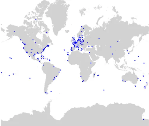
Our starting dataset are the weekly terrestrial frame solutions provided by the IGS in the frame of its second reprocessing campaign (repro2; Rebischung et al., 2016). Each weekly solution includes the coordinates of a global station network, expressed in the IGb08 reference frame (Rebischung, 2012), and the full covariance matrix of the station coordinates in SINEX format (IERS, 2006). The weekly IGS repro2 solutions were obtained by stacking the daily coordinate solutions provided by eight different IGS Analysis Centers, then forming weekly averages of the daily combined solutions. A list of the models and conventions used in the repro2 campaign can be found at http://acc.igs.org/reprocess2.html. Their consistent application by the Analysis Centers guarantees the homogeneity of the combined solutions over the whole repro2 period. Among all stations available in the repro2 dataset, we selected a subset of 195 stations (Fig. 1) based on the following criteria: - minimum time series length of 3 years, as recommended by Lavallée and Blewitt (2002) for the estimation of reliable velocities, - absence of inter-annual trends or transient events (in particular post-seismic displacements),

- minimum time span between two successive discontinuities set to a few weeks (segment with a few points are eliminated).

(5)

3 Methodology

The IGS repro2 dataset includes daily 3-dimensional positions over more than 20 years for more than 1000 stations. If one wants to form the covariance matrix of this whole dataset based on a generic spatiotemporal correlation model, such as in Amiri-Simkooei (2009), its size would be as large as 1000x(20x365)x3 (about 22 millions). A weighted least-squares adjustment of the station velocities would require inverting such a matrix, which is not practically feasible. Using a Kalman filter instead avoids forming and inverting this full covariance matrix. However, a Kalman filter is applicable to finite-order Markov processes only. Flicker noise is not such a process and therefore needs to be approximated, as was done in previous studies carried out in the same context (Dong et al., 1998; Wu et al., 2015). In this section, we describe the methodology that we used to determine a spatio-temporal correlation model for GNSS station coordinate variations adapted to the Kalman filter framework. 3.1 Kalman filter A Kalman filter is an algorithm which allows estimating parameters that follow a state-space model (Kalman, 1960). In such a model, the vector of unknown parameters Xt varies with time following a

state equation: the vector Xt+1 at epoch t+1 can be deduced from the vector Xt at epoch t by applying

a linear operator and adding a white process noise:

𝑋!!!= 𝐿!𝑋!+ 𝐴! (eq 1)

(6)

The uncorrelated noise term At models the deviation from this linear model. It is assumed to be

normally distributed with zero mean and a known covariance matrix Tt. The parameters at epoch t are related to the vector of observations Yt at time t by a linear operator and another additive normally distributed white noise term Bt with zero mean and known covariance matrix Mt: 𝑌! = 𝐻!𝑋!+ 𝐵! (eq 2)

The vector of parameters Xt can be estimated at every epoch t using all available observations

following a first forward calculation and a backward smoothing. The details of the algorithm can be found for example in Herring et al. (1990) who summarized all useful information from both theoretical and practical aspects. 3.1.1 Kinematic model for station coordinates For any East, North or Up component k of the coordinate time series of station l, we adopted the following kinematic model for station coordinate variations xk,l(t): 𝑥_!,! 𝑡 = 𝑥_!,!! _{+ 𝑡 − 𝑡} ! 𝑣!,!! + 𝛿 ! 𝑥_!,!;!𝐻 𝑡 − 𝑡_!,!;! + 𝑡 − 𝑡_! ! 𝛿𝑣_!,!;!𝐻 𝑡 − 𝑡_!,!;! + 𝑎!,!;!𝑐𝑜𝑠 2𝜋𝑓𝑡 + 𝑏!,!;!𝑠𝑖𝑛 2𝜋𝑓𝑡 ! + 𝑧!,! 𝑡 + 𝛽!,!𝜀!,!!" 𝑡 (eq 3) with the following parameters to be estimated and included in the state vector: • xk,l0, vk,l0 : reference position and velocity at epoch t0 • δxk,l;i, δvk,l;j : offsets to the reference position and velocity in case of discontinuities. • ak,l;f and bk,l;f : amplitudes of a constant periodic signal at frequency f.

The position and velocity discontinuity dates tk,l;i and tk,l;j are taken from the catalog provided by Altamimi et al. (2016). H(t) denotes the Heaviside function which is zero for negative arguments and one for positive arguments. Finally, the set of frequencies f is chosen to include, for all stations, the annual and semi-annual frequencies, but also the first seven harmonics of the GPS draconitic frequency, which were found in a spectral analysis of the IGS repro2 time series by Rebischung et al. (2015). This kinematic model is valid for stations far from earthquake epicenters. However, it is still possible to add post-seismic deformation model parameters as done by Altamimi et al. (2016). The last two terms of equation 3 respectively represent the temporally correlated and uncorrelated noise in the coordinate time series.

εk,lVW(t) is a variable white noise term with zero mean and variance taken from the covariance

matrices of the IGS repro2 weekly solutions. We introduce spatial correlations by also using the inter-station and inter-component terms of the covariance matrices of the IGS repro2 weekly solutions. This noise term aims at representing random observational errors in the coordinate time series, whose spatial structure is supposedly well described by the covariance matrices resulting from the adjustment of the IGS repro2 weekly solutions. We however keep the possibility of rescaling those covariance matrices by factors β²k,l that may depend on the station and component.

(7)

6 Benoist et al., spatiotemporal correlations of GNSS coordinate time series, submitted to Journal of geodynamics Finally, zk,l(t) is the spatio-temporally correlated noise that we aim at modeling and introduce into the adjustment of station velocities. It is described in the next section. 3.1.2 Time-correlated noise It is well known that a flicker noise model generally best describes the time-correlated noise in GNSS coordinate time series (Williams et al., 2004; Santamaría-Gómez et al., 2011). Flicker noise can however not be represented by a finite-order state model, hence in a Kalman filter framework (Brown, 1984). On the other hand, simpler time-correlated noise models such as auto-regressive (AR) processes can easily be incorporated in a Kalman filter, as they can be represented by a finite state equation. The simplest AR process is the first-order auto-regressive process (AR(1)). We model the time-correlated noise zk,l(t) in component k of the coordinate time series of station l, by such an

AR(1) process but imposing a positive coefficient 𝜑k,l in the linear first-order difference equation. It satisfies the following equation: 𝑧_!,! 𝑡 + 𝑑𝑡 = 𝜑_!,!𝑧_!,! 𝑡 + 𝑢_!,! 𝑡 + 𝑑𝑡 = 𝑒 !!" !!,!_𝑧_!,! _{𝑡 + 𝑢}_!,! _{𝑡 + 𝑑𝑡} _(eq 4) where uk,l(t), called innovation, is a white noise process the variance of which is given by 𝑣𝑎𝑟 𝑢!,! 𝑡 = 𝜎!,!! 1 − 𝑒 !!!" !!,! _(eq 5) and dt the time interval between two successive coordinate epochs. This process _z k,l(t) has a variance

σ²k,l and an autocorrelation function which decreases exponentially with a time decay τk,l. As opposed

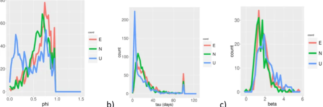
to a random walk, an AR(1) process is stationary. Besides, the expected value of the prediction of such AR(1) process tends to zero, which is a useful property in the context of terrestrial reference frame definition, as reference station coordinates are usually extrapolated for operational applications. We adjusted to each individual station coordinate time series and component xk,l(t) the deterministic coefficients of equation 3 as well as the white noise variance and the AR(1) parameters (σ²k,l, 𝜑k,l). The estimation has been made by maximum likelihood using the Hector software (Bos et al., 2013) and has been carried out on IGS daily station coordinate time series. The empirical distribution of the 𝜑k,l coefficients, converted to a weekly sampling rate, is shown in Fig. 2a. The corresponding decay times τk,l are shown in Fig. 2b. To facilitate the modeling of spatial correlations and because it can be observed in Fig. 2 that this approximation is not unreasonable, a single median value of τ = 19.7 days will be used in the following for all stations and components.

To ensure consistency of the other parameters with this choice, we then re-estimated an AR(1) process variance σ²k,l and a variable white noise standard deviation scaling factor βk,l for each station

and component, with the AR(1) decay time τk,l fixed to 19.7 days for all stations and components. Fig.

2c shows the estimated variable white noise scaling factors βk,l. These factors aim to rescale the

standard deviations of the coordinates that have been extracted from the IGS repro2 SINEX files. The estimated scaling factors are significantly larger than one (median values are 1.7, 1.5 and 2.0 in the East, North and Up components). As a consequence, we choose in the following to rescale the SINEX file covariance matrices. For that purpose, either the station- and component-specific standard deviation scaling factors βk,l will be used, or their median value β = 1.7 for all stations and

components.

(8)

a) b) c)

Fig. 2 Histograms of the a) estimated ϕk,l coefficients. b) corresponding decay times τk,l. c) estimated variable white noise standard deviation scaling factors βk,l with AR(1) decay time τk,l fixed

to 19.7 days. The parameters estimated for each component are shown with different colors: East in red, North in green, Up in blue.

3.1.3 Kalman filter implementation

The vector of parameters Xt (state vector) in equations 1 and 2 is composed of the deterministic

parameters listed in equation 3 and of the AR(1) process value zk,l(t) for every station and

component. The vector of observations includes the input GNSS positions. 𝑋_! = ⋯ 𝑥_!,!! _{⋯ ⋯ 𝑣} !,!! ⋯ ⋯ 𝛿𝑥!,!:!⋯ ⋯ 𝛿𝑣!,!:!⋯ ⋯ 𝑎!,!;!⋯ ⋯ 𝑏!,!;!⋯ ⋯ 𝑧!,! 𝑡 ⋯ ! (eq 6) 𝑌! = ⋯ 𝑥!,! 𝑡 ⋯ ! In equation 6, the ellipsis stands for parameter repetition over all indices k, l and f when relevant. It is worth mentioning that this state representation is not unique. We build the observation design matrix Ht in accordance with this particular representation. The state transition matrix Lt is diagonal,

with diagonal terms equal to 1 for the deterministic parameters and to e-dt/τ_{for the AR(1) processes}

with

τ

identical for all stations and components.

The observation errors Bt in equation 1 correspond to the variable white noise term εk,lVW(t) in

equation 3. As already mentioned, its spatial correlations are accounted for by using the full, rescaled covariance matrices from the IGS repro2 SINEX files as Mt = var(Bt).

Finally, the spatial correlations of the AR(1) processes are accounted for via the covariance matrix Tt of the process noise At. Several possible choices for Tt = var(At) will be tested and presented in section 3.3. In our model, no spatial correlation is introduced between the deterministic parameters of different stations such as trends and periodic signals. See discussion in section 5. 3.2 Spatial correlation study

We aim to assess the spatial correlations of the time-correlated noise in the selected station coordinate time series, and thus to evaluate different models for Tt = var(At). We choose to adopt a

(9)

separately. Secondly, we assess the correlations between obtained series in order to easily fill matrix Tt.

In the first step, a Kalman filter and smoother based on the previous equations was applied independently to each station and component. The AR(1) innovation variance (eq 5) previously estimated by maximum likelihood was used as the one-dimensional process noise variance Tt =

var(At). The one-dimensional variance of the observation errors Mt = var(Bt) was obtained by

multiplying the formal observation variances from the IGS repro2 SINEX files by the previously estimated factor βk,l2.

The innovations of the AR(1) process estimates obtained from those station- and component-specific Kalman filters were then analyzed and used to build different models of their spatial correlation. In section 3.2.1, we start by describing our approach to rigorously compute spatial covariances of a 3-dimensional field on a sphere. In Section 3.2.2, we then present spatial semi-variograms of the estimated AR(1) process normalized innovations. 3.2.1 Frame Coordinate time series are usually studied in the topocentric frame (East, North, Height), hereafter denoted ENH. This frame is however undefined at the poles. Besides, the (East, North) frames of a pair of stations at high latitudes may be relatively oriented in any way: certain pairs of stations may have parallel East and North directions, while others may have opposite East and North directions. Comparing the displacements of station pairs in their ENH frames has therefore no “absolute” meaning.

We introduce a local frame, hereafter denoted UVH, in which the displacements of any station pair can be meaningfully compared. Let A and B be two points on a sphere, see figure 3. At point A, we define a direct orthonormal frame 𝑢!, 𝑣!, ℎ! where 𝑢! is oriented from A to B along the great

circle linking the two points, ℎ! is normal to the sphere and 𝑣! complements the direct orthonormal

frame. Similarly, at point B, we define a direct orthonormal frame 𝑢!, 𝑣!, ℎ! where 𝑢! is tangent

to the great circle linking A and B, ℎ! is normal to the sphere and 𝑣! completes the direct

orthonormal frame. This UVH frame has the advantage that, in spherical geometry, the U and V directions of a pair of points are always parallel to each other. The U and V directions can be interpreted as the directions of dilatation/compression and shear deformation between any two points. Fig. 3: UVH frame and angle convention.

(10)

Let αA denote the azimuth (counted from North) from A to B and αB denote the azimuth from B to A

minus π. The displacements of points A in the UVH frame can be deduced from the displacements in their ENH frames by the following relationships: 𝑢_! 𝑣_! ℎ_! = 𝑅 𝛼! 𝑒_! 𝑛_! ℎ_! (eq 7) where R defines a rotation in the tangent plane to the sphere: 𝑅 𝜃 = −𝑐𝑜𝑠 𝜃𝑠𝑖𝑛 𝜃 𝑐𝑜𝑠 𝜃𝑠𝑖𝑛 𝜃 00 0 0 1 (eq 8)

The same equation holds for B (replace αA by αB). The covariance of the point displacements in their

UVH frames is thus related to the covariance of their ENH displacements by: 𝑐𝑜𝑣 𝑢! 𝑣_! ℎ_! 𝑢! 𝑣_! ℎ_! = 𝑅 𝛼₀! _{𝑅 𝛼}0 ! 𝑐𝑜𝑣 𝑒! 𝑛_! ℎ_! 𝑒! 𝑛_! ℎ_! 𝑅 𝛼_! ! ₀ 0 𝑅 𝛼! ! (eq 9) 3.2.2. Semi-variograms To study the spatial correlations of the time-correlated noise in the selected station coordinate time series, we formed semi-variogram clouds of the time series of AR(1) innovations uk,l(t) described in the introduction of section 3.2, after normalizing them by their standard deviations from equation 5 to derive normalized innovations 𝑢k,l(t). For each pair of components (k’1, k’2) in the UVH frame and

each pair of stations (l1, l2), we thus computed the sample variance over time t of the differences

between the time series of normalized AR(1) innovations 𝑢k’1,l1(t) and 𝑢k’2,l2(t). The semi-variogram

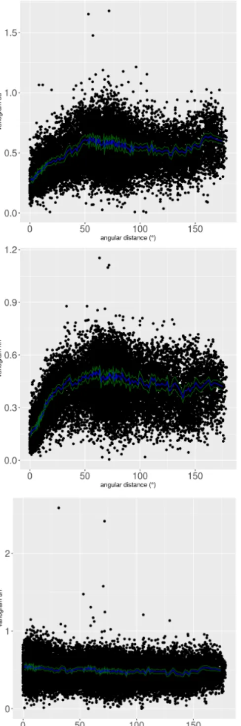
clouds, represented by black dots in Fig. 4, display those sample variances scaled by a factor 1/2 as a function of the distance between each pair of station, separately for each component pair UU, VV, HH, UV, UH and VH. The distance is computed on the sphere that is why it is provided in degrees in the following.

Sample semi-variograms (blue lines in Fig. 4) were then obtained by computing mean half sample variances over distance classes of 1000 elements. 95% confidence intervals of the sample semi-variograms (green lines in Fig. 4) were estimated using the bootstrap method. _{It is worth reminding}

that in case of a stationary process, the theoretical semi-variogram at a distance d equates the variance of the process minus its covariance at d which explains the conventional ½ scaling factor previously used to compute the semi-variogram clouds and sample semi-variograms from sample variances.

In the V and H components, the semi-variograms flatten out after an angular distance of approximately 60°. The semi-variogram in the U component has a less typical behavior, as it reaches a maximum at around 60°, after which correlation increases until about 130°, then decreases again. The cross-semi-variograms between components (i.e., UV, UH and VH in Fig. 4) are flat, indicating the

(11)

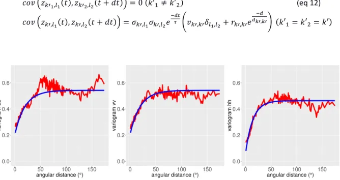
absence of spatial cross-correlation between components, which was also observed by Amiri-Simkooei et al. (2017). The asymptotic values of all sample semi-variograms are about 0.5. This means that the sample variances of the AR(1) innovation time series obtained from our station- and component-specific Kalman filters are in average twice smaller than the AR(1) innovation variances previously estimated by maximum likelihood. A simple simulation was conducted by generating an AR(1) plus white noise time series with similar variance levels as our series. After estimation of the AR(1) time series using a Kalman filter, we found that the empirical variance of smoothed AR(1) time series filter was indeed twice smaller than the true level which explains this under-estimation. Simple distance-dependent covariance models were then adjusted to the intra-component (UU, VV and HH) sample semi-variograms. We chose to model them by the sum of nugget effects and of exponential functions of the distance. This is a classical choice in geostatistics, which fits quite well the sample semi-variograms (see Fig. 5). For a given component k' = (u,v,h) and any two stations l1, l2 separated by a distance d, the covariance of the normalized AR(1) innovations is thus modelled by: 𝑐𝑜𝑣 𝑢_!!,!! 𝑡 , 𝑢_!!,!! 𝑡 = 𝑣_!!,!!𝛿_!!,!!+ 𝑟_!!,!!𝑒 !! !!!,!! _(eq 10)

The parameters νk’,k’, rk’,k’, dk’,k’ of those covariance models were adjusted to the sample

intra-component semi-variograms by non-linear least squares. Their values are given in Table 1. They account for the asymptotic values of the semi-variograms which is not 1 for self-consistency with the estimator used, see the discussion in section 5. The adjusted models are compared to the sample semi-variograms in Fig. 5. Note that a single covariance model was simultaneously adjusted to both horizontal (UU and VV) semi-variograms.

We chose to model cross-component semi-variograms by constant values, which comes to setting the cross-component covariances to 0: 𝑐𝑜𝑣 𝑢!!!,!! 𝑡 , 𝑢!!!,!! 𝑡 = 0 𝑘′!≠ 𝑘′! (eq 11)

(12)

11 Benoist et al., spatiotemporal correlations of GNSS coordinate time series, submitted to Journal of geodynamics Fig. 4 Variogram clouds (black dots) and sample semi-variograms of the normalized innovations of the AR(1) process estimates (blue curves) obtained from station- and component-specific Kalman filters with their 95% confidence intervals (green curves).

(13)

12 Benoist et al., spatiotemporal correlations of GNSS coordinate time series, submitted to Journal of geodynamics Component pair k’1, k’2 νk’1,k’2 rk’1,k’2 dk’1,k’2 (°) U,U and V,V 0.21 0.33 17.6 H,H 0.06 0.40 14.1 Table 1 Parameters of the adjusted spatial covariance models We have now effectively built a full spatiotemporal covariance model for the time-correlated noise

zk’,l(t) in the selected station coordinate time series. With the temporal representation of zk’,l(t) as

AR(1) processes and the nugget [+ exponential] spatial covariance models derived above, the covariance between the time-correlated noise in any two components k’1, k’2 at any two stations l1, l2 separated by a distance d and any two epochs t, t+dt can indeed be obtained by: 𝑐𝑜𝑣 𝑧!!!,!! 𝑡 , 𝑧!!!,!! 𝑡 + 𝑑𝑡 = 0 𝑘′! ≠ 𝑘′! (eq 12) 𝑐𝑜𝑣 𝑧!!,!! 𝑡 , 𝑧!!,!! 𝑡 + 𝑑𝑡 = 𝜎!!,!!𝜎!!,!!𝑒 !!" ! 𝑣_!!,!!𝛿_! !,!!+ 𝑟!!,!!𝑒 !! !!!,!! _𝑘′_!_{= 𝑘′}_!_{= 𝑘′} Fig. 5 Red: intra-component sample semi-variograms (same as in Fig. 4). Blue: adjusted “nugget + exponential” models. 3.3 Tested covariance models The spatiotemporal covariance model derived in the previous section allows to populate the process noise covariance matrix Tt = var(At) in a multi-station Kalman filter, hence to account for spatial

correlations of the time-correlated noise zk,l(t) in the determination of the velocities of a station

network. Results based on this covariance model will be presented in the next section and compared to the results obtained with two alternative covariance models for zk,l(t). A first alternative model

(14)

where no spatial correlations are introduced (i.e., in which Tt is diagonal) will be used as a control

model. In the second alternative model, the nugget [+ exponential] spatial covariance models will be replaced by covariances specific to each station and component pair. Namely, the empirical covariances between the time series of normalized AR(1) innovations previously derived for each station and component separately will be used in place of equations 10 and 11. The aim of this second alternative model is to assess whether a complex station-pair-adapted spatial covariance model may provide improvements over simple distance-dependent covariance models.

Different options will also be tested for the covariance matrices Mt = var(Bt) of the observation

errors. They will be taken as either:

(a) diagonal matrices with diagonal entries equal to the formal observation variances from the IGS repro2 SINEX files multiplied by the previously estimated station- and component-specific factors βk,l2. The spatial correlations of the variable white noise εk,lVW(t) are in this case neglected;

(b) the full SINEX covariance matrices rescaled by a single median factor of β2 _{(see section 3.1.2);}

(c) the full SINEX covariance matrices rescaled by station- and component-specific factors. In this case, each entry sk1l1,k2l2 of the original SINEX covariance matrices (after they have been rotated to

the station ENH frames) is replaced by βk1,l1βk2,l2 sk1l1,k2l2.

Four different models will be tested in total (Table 2). In the model called WoSC (without spatial correlations), the spatial correlations of both zk,l(t) and εk,lVW(t) are neglected (i.e., Tt and Mt are

diagonal). Using this model in a multi-station Kalman filter is equivalent to running independent Kalman filters for each station and component separately. The next two models, WSC-EMP-MULTI-BETA and WSC-EMP-ONE-BETA, use empirical covariances specific to each station and component pair to account for the spatial correlations of zk,l(t). They also both account for the spatial correlations

of the observation errors by using full covariance matrices Mt = var(Bt). They only differ by the way

the SINEX covariance matrices are rescaled to form Mt: either by station- and component-specific

factors βk1,l1βk2,l2, or by a single median factor β2. Finally, the last model WSC-DIST accounts for the

spatial correlations of zk,l(t) via the nugget [+ exponential] spatial covariance models derived above,

and for the spatial correlations of εk,lVW(t) via full SINEX covariance matrices rescaled by station- and

component-specific factors βk1,l1βk2,l2.

Model name Spatial Variable white noise Time-correlated noise

correlations factor(s) Scaling correlations Spatial Spatial covariance model

WoSC no specific βk,l’s no -

WSC-EMP-MULTI-BETA yes specific βk,l’s yes empirical covariances

WSC-EMP-ONE-BETA yes median β yes empirical covariances

WSC-DIST yes specific βk,l’s yes nugget [+exp] _model

Table

2

: Compared covariance models. See text for detailed explanations.

4 Results

This section presents the results of multi-station Kalman filters and smoothers for two test datasets of 10 and 11 stations, using the four spatiotemporal covariance models listed in Table 2. The different models are compared via two complementary approaches: firstly, by evaluating the

(15)

interpolation abilities of the models by cross-validation; secondly, by evaluating the accuracy of station velocities estimated from short time series.

4.1 Datasets

Two clusters of stations have been selected in Europe and in the USA to assess the covariance models presented in section 3. They consist of 10 or 11 nearby stations each, with long time series and few data gaps. Fig. 6a) and Fig. 6c) show the distribution of the selected stations. The relaxation distance of the semi-variogram in the vertical component is 14.1° according to Table 1. With such a value, the covariance of the process noise drops to half its variance for a distance of 9.8°. This corresponds to the typical size of our network. Thus, due to the density of the network, it is expected that the modelling of spatio-temporal correlation impacts our results. Fig. 6b) and Fig. 6d) show the time spans of their time series. Data gaps are clearly visible for some stations.

(16)

F

ig.

6

: a) Distribution of the 10 selected stations in Europe . b) Time spans of their repro2 coordinate time series. The 1-year periods used for cross-validation (see section 4.2) are shown in red. c) Distribution of the 11 selected stations in the USA (red dots) among the previously selected repro2 stations (black dots). d) Time spans of their repro2 coordinate time series. The 1-year periods used for cross-validation (see section 4.2) are shown in red.

4.2 Cross-validation

Cross-validation consists in removing a subset of data from the available dataset while adjusting a model. The adjusted model is then used to predict the removed data. Comparison of the values predicted by the model with the actual removed observations allows testing the predictive capacity of the model.

For each test dataset, we thus sequentially removed one year of data from each station position time series (see Fig. 6b) and Fig. 6d)). Multi-station Kalman filters based on the various spatiotemporal covariance models listed in Table 2 were then used to predict the removed observations. The purpose of this test was to verify that, when accounting for spatial correlations, the coordinate

a)

b)

c)

d)

(17)

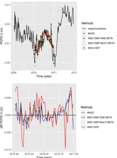
16 Benoist et al., spatiotemporal correlations of GNSS coordinate time series, submitted to Journal of geodynamics predictions made for a particular station benefit from the observations of neighboring stations. Note that in case where empirical spatial covariances were used (for models WSC-EMP-MULTI-BETA and WSC-EMP-ONE-BETA), those empirical covariances were estimated without using the removed data period of the considered station. As an illustation, Fig. 7a) shows the original, detrended height time series of station POTS (Potsdam, Germany) and the predictions obtained for the test year 2010 with the various spatiotemporal covariance models listed in Table 2. Fig. 7b) shows the differences between those various predictions and the original observations. The WoSC model (equivalent to a single-station Kalman filter) predicts the original series based on a purely kinematic model, i.e. on periodic functions and on the AR(1) forecast which tends to zero. All the other models, which account for spatial correlations of the time-correlated noise, yield better predictions of the original data. This example illustrates that, when accounting for spatial correlations, the coordinate predictions made for a particular station can actually benefit from the observations of neighboring stations. Tables 3 and 4 provide the RMS of the differences between the predictions obtained with the various spatiotemporal covariance models and the original observations for each of the two selected subsets of stations. It can first be noticed that the different covariance models used for the variable white noise have little impact on the cross-validation results since using a single or multiple variable white noise scaling factors (WSC-EMP-ONE-BETA vs. WSC-EMP-MULTI-BETA) leads to identical statistics. We could also verify (not shown here) that accounting or not for the spatial correlations of the variable white noise has no impact on the cross-validation results.

On the other hand, the three models that account for spatial correlations of the time-correlated noise (WSC-EMP-ONE-BETA, WSC-EMP-MULTI-BETA, WSC-DIST) lead to substantially better predictions than our control model WoSC. Those three models perform quite similarly in both horizontal components. In the vertical component however, the WSC-DIST model (i.e. simple nugget + exponential spatial covariance models) performs slightly better than the one which makes use of empirical spatial covariances. This may be explained by the significantly higher number of parameters estimated for models WSC-EMP-ONE-BETA and WSC-EMP-MULTI-BETA models. They cause a better fit of the model to used dataset but a poorer ability to predict values.

(18)

17 Benoist et al., spatiotemporal correlations of GNSS coordinate time series, submitted to Journal of geodynamics Fig. 7: a) Original detrended height time series (black) of station POTS (Postdam, Germany) compared to the predictions obtained with various spatiotemporal covariance models. b) Differences between the various predictions and the original time series. Note that in both plots, the results of the two models WSC-EMP-ONE-BETA and WSC-EMP-MULTI-BETA are superimposed. E (mm) N (mm) U (mm) WoSC 1.0 1.0 3.7 WSC-EMP-ONE-BETA 0.7 0.7 2.7 WSC-EMP-MULTI-BETA 0.7 0.7 2.7 WSC-DIST 0.7 0.7 2.5

Table 3: RMS of the differences between the predictions obtained with various spatiotemporal covariance models and the original coordinate time series for the 10 selected stations in Europe

(19)

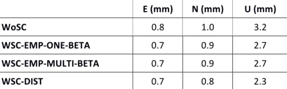
18 Benoist et al., spatiotemporal correlations of GNSS coordinate time series, submitted to Journal of geodynamics E (mm) N (mm) U (mm) WoSC 0.8 1.0 3.2 WSC-EMP-ONE-BETA 0.7 0.9 2.7 WSC-EMP-MULTI-BETA 0.7 0.9 2.7 WSC-DIST 0.7 0.8 2.3

Table 4: RMS of the differences between the predictions obtained with various spatiotemporal covariance models and the original coordinate time series for the 11 selected stations in the USA

4.3 Impact on velocities estimated from short time series

Time-correlated noise generates variations in GNSS station coordinate time series that affect the estimation of station velocities. Velocities estimated from short time series are particularly impacted. These time-correlated variations are however spatially correlated, and it can be expected that, when accounting for these spatial correlations, velocities estimated from short time series may benefit from the longer time series of nearby stations. The experiment described in this section demonstrates that this is actually the case.

To evaluate the impact of accounting for spatial correlations on velocities estimated from short time series, a reference velocity r was first computed independently for each of the 10 or 11 stations in each test dataset, using its full time series. Then, for each station successively, new velocity estimates were obtained from different multi-station Kalman filters in which the full time series of the neighboring stations were used, but only the 100 first weekly positions of the considered station. A velocity r̂0 was thus derived from a Kalman filter based on the WoSC covariance model (equivalent to

a single-station filter based on the truncated time series). Two other velocity estimates r̂EMP and r̂DIST

were obtained from Kalman filters based on the WSC-EMP-MULTI-BETA and WSC-DIST covariance models respectively. It was expected that, compared to r̂0, those two estimates would benefit from

the long time series of the nearby stations and would hence be closer to the reference velocity r.

Another possible approach to remove spatially correlated errors while estimating station velocities is spatial filtering. For comparison with our approach, we compute another velocity estimate r̂SF from

each truncated time series using the basic spatial filtering technique which consists in removing a mean regional residual signal from the considered time series. As the variance of noise processes is larger in the vertical component, only the results obtained on the vertical component will be detailed here. The differences between the various velocity estimates obtained from truncated station coordinate time series and the reference velocities r are provided in Table 5. It can be noticed that the velocity errors reported in columns 4 are generally smaller when spatial correlations between coordinate series are introduced using our nugget [+ exponential] spatial covariance model. This is not the case, however, when spatial correlations are modeled using empirical covariances. This is likely because the empirical covariances estimated between the truncated series, which has only 100 points, and the other series may not be reliable.

The last column of Table 5 provides the velocity errors obtained when using a spatial filtering technique. Compared to our new method based on the model WSC-DIST, spatial filtering leads to similar average velocity errors. Our conclusion is that our nugget [+ exponential] covariance model

(20)

19 Benoist et al., spatiotemporal correlations of GNSS coordinate time series, submitted to Journal of geodynamics allows reducing biases in velocities estimated from short time series, and that it shows in average similar performance to standard spatial filtering in this test. The same analysis has been carried out for the horizontal components. The mean absolute horizontal velocity errors over USA are 0.33 mm/yr and 0.37 mm/yr for the WSC-DIST and WSC-EMP-MULTI-BETA covariance models respectively against 0.40 mm/yr when no spatial correlation is assumed. Over Europe, the values are 0.54 mm/yr and 0.65 mm/yr against 0.62 mm/yr respectively. While the empirical covariance model provides worst mean statistics for Europe, more than 3 series over 4 show similar or best performances compared to the standard approach. Whatever the covariance model used, there are always more series that show improvement than degradation but the magnitude of the improvement is moderate. The benefit of using the new approach is smaller on the horizontal components. |r̂0 - r| |r̂EMP - r| |r̂DIST - r| |r̂SF - r| GRAS 0.58 0.38 0.42 2.06 GRAZ 3.55 3.54 2.84 2.34 MARS 0.25 0.13 0.25 0.11 POTS 5.76 5.97 4.14 3.28 WROC 1.3 1.22 0.82 1.09 WTZA 0.33 0.20 0.46 1.92 WTZS 1.57 1.49 0.51 0.40 WTZZ 1.70 1.37 1.38 1.71 ZIMJ 0.81 0.98 1.14 1.39 ZIMM 1.25 1.39 0.08 0.01 Europe 2.35 2.38 1.73 1.74 ANP1 0.25 0.15 0.30 0.88 CASL 2.90 2.95 1.96 0.33 GLPT 0.00 0.45 1.58 1.57 GODE 0.75 0.70 1.03 0.18 NJI2 0.20 0.19 0.09 0.88 SAV1 0.30 0.17 0.03 1.19 TN22 1.27 1.23 0.63 0.51 USN3 2.49 2.26 1.06 2.09 VIMS 1.11 1.19 1.80 0.63 VTSP 2.34 2.44 1.27 1.25 WES2 1.45 1.44 1.06 0.78 USA 1.53 1.52 1.16 1.08 mean 1.96 1.97 1.45 1.43

(21)

Table 5: Absolute differences (mm/yr) between vertical velocity estimates obtained from truncated station coordinate time series using different strategies to account for spatial correlations and reference vertical velocities r. See text for detailed explanations. The rows “Europe” and “USA” contain quadratric mean vertical velocity differences for the stations in each test dataset. The last row contains global averages for all the 21 stations. Values are written in bold when the velocity estimates is equal or closer to the reference velocity r than the basic estimate r̂0 that ignores spatial correlations.

5 Discussion

We have developed a methodology to account for spatiotemporally correlated noise in a Kalman-filter-based determination of GNSS station velocities. A variable white noise model was used to represent the temporally uncorrelated noise in station coordinate time series, with a spatial structure represented by the full, rescaled covariance matrices provided with the IGS repro2 weekly solutions. Time-correlated noise was represented by AR(1) processes, as an approximation to the standard flicker noise model. Two models of the spatial covariances of the AR(1) processes have been constructed and evaluated. A simple distance-dependent nugget [+ exponential] model has first been adjusted to sample semi-variograms obtained from a global network of 195 stations. Those sample semi-variograms have been derived in a specific frame in which covariances between station horizontal displacements can be meaningfully evaluated. While our approach is more rigorous, it confirms the findings of Amiri-Simkooei et al. (2017): intra-component spatial correlations exist up to distances of a few thousands of kilometers, while there are no significant cross-component correlations. The second considered spatial covariance model makes use of station-pair-specific empirical covariances.

To evaluate those two spatial covariance models, we used two test datasets of 10 and 11 stations in Europe and in the USA. Both models have been shown to perform better for interpolating coordinates than standard models that ignore spatial correlations. Moreover, the distance-dependent nugget [+ exponential] model leads to better results for the vertical component than the model based on empirical covariance estimates. Based on simulations conducted over the same dataset, it was shown that vertical velocities estimated from short time series generally benefit from modeling spatiotemporal correlations when using the distance-dependent nugget [+ exponential] spatial covariance model, with similar average performance as standard spatial filtering.

We made use of a two-step approach to determine the spatial dependency of GNSS series modeled as AR(1) processes. In section 3.2.2, we found that our derived empirical semi-variograms under-estimate the variance level of the series. This shows that our two-step approach to assess the spatial dependencies of our series based on an AR(1) assumption is probably not optimal. However, the cross-validation analyses that we performed showed that our spatial-dependent model, even if not optimal, is superior to a model assuming no spatial correlation of the time-correlated noise. This first study tends to show that modeling spatial dependencies benefits to terrestrial reference frame determination.

For future work, we recommend to investigate refined models of temporal correlations that better approximate flicker noise than AR(1) processes. A realistic modeling of temporal correlations is indeed crucial for assessing the precision of the estimated station velocities (e.g., Williams, 2003). Besides, to further strengthen the estimation of station velocities, advantage could additionally be

(22)

taken of the spatial correlations of periodic station motions. Seasonal station motions have indeed been shown to be spatially correlated (Dong et al., 2002; Collilieux et al., 2007). Since seasonal station motions affect the estimation of station velocities from short time series (Blewitt and Lavallée, 2002), it can thus be expected that accounting for their spatial correlations will improve even more velocity estimates.

Acknowledgment

We thank Etienne Bernard for his advice when defining the frame UVH used in this study and the two anonymous reviewers for their valuable comments. This study contributes to the IdEx Université de Paris ANR-18-IDEX-0001. It is partly supported by the Agence Nationale de la Recherche (ANR) project « Geodesie » ANR-16-CE01-0001.

Data Availability

Data used in this study have been provided by the IGS (Dow et al., 2009) and are available online, for example at the CDDIS FTP web site: ftp://cddis.gsfc.nasa.gov/pub/gps/products/ or the IGN data center ftp://igs.ensg.ign.fr/pub/igs/products/. For each GPS week WWWW, data are available in the repertory WWWW/repro2/.

References

Altamimi, Z., Rebischung, P., Métivier, L., Collilieux, X., 2016. ITRF2014: A new release of the International Terrestrial Reference Frame modeling nonlinear station motions, J. Geophys. Res. 121(B8):6109-6131, doi:10.1002/2016JB013098.

Amiri-Simkooei, A.R., 2009. Noise in multivariate GPS position time-series, J. Geodesy 83, 175-187, doi:10.1007/s00190-008-0251-8.

Amiri-Simkooei, A.R., Mohammadloo, T. H., Argus, D., 2017. Multivariate analysis of GPS position time series of JPL second reprocessing campaign, J. Geodesy 91, 685-704, doi:10.1007/s00190-016-0991-9. Blewitt, G., D. Lavallée (2002). Effect of annual signals on geodetic velocity. J. Geophys. Res. 107(B7), doi:10.1029/2001JB000570. Bos, M. S., Fernandes, R. M. S., Williams, S. D. P., Bastos, L., 2013. Fast error analysis of continuous GNSS observations with missing data. J. Geodesy, 87(4), 351-360, doi:10.1007/s00190-012-0605-0

Brown, R.G., 1984. Kalman filter modeling. Proceedings of the Sixteenth Annual Precise Time and Time Interval (PTTI) Applications and Planning Meeting, Greenbelt, USA, 27-29 Nov. Chanard, K., Fleitout, L., Calais, E., Rebischung, P., Avouac, J.P. 2018. Toward a global horizontal and vertical elastic load deformation model derived from GRACE and GNSS station position time series. J. Geophys. Res. 123(4), 3225-3237, doi:10.1002/2017JB015245.

Chen, Q., van Dam, T.M., Sneeuw, N., Collilieux, X., Weigelt M., Rebischung, P. 2013 Singular spectrum analysis for modeling seasonal signals from GPS time series, J. Geodynamics 72:25-35, doi:10.1016/j.jog.2013.05.005.

(23)

22 Benoist et al., spatiotemporal correlations of GNSS coordinate time series, submitted to Journal of geodynamics Collilieux, X., Lebarbier, E., Robin, S., 2018. A factor model approach for the joint segmentation with between-series correlation, Scand. J. Stat., doi:10.1111/sjos.12368. Collilieux, X., van Dam, T., Ray, J., Coulot, D., Métivier, L., Altamimi, Z., 2012. Strategies to mitigate aliasing of loading signals while estimating GPS frame parameters, J. Geodesy 86(1), 1-14, doi:10.1007/s00190-011-0487-6.

Collilieux, X., Altamimi, Z., Coulot, D., Ray, J., Sillard, P., 2007. Comparison of very long baseline interferometry, GPS, and satellite laser ranging height residuals from ITRF2005 using spectral and correlation methods, J. Geophys. Res. 112, B12403, doi:10.1029/2007JB004933.

Davis, J.L., Elósegui, P., Mitrovica, J.X., Tamisiea, M.E., 2004. Climate-driven deformation of the solid Earth from GRACE and GPS. Geophysical Research Letters, 31(24), doi:10.1029/2004GL021435.

Dong, D., Fang, P., Bock, Y., Webb, F.H., Prawirodirdjo, L., Kedar, S., Jamason, P., 2006. Spatiotemporal filtering using principal component analysis and Karhunen-Loeve expansion approaches for regional GPS network analysis, J. Geophys. Res., B10, 3405-+, doi:10.1029/2005JB003806 Dong, D., T.A. Herring, R.W. King, 1998. Estimating regional deformation from a combination of space and terrestrial geodetic data, J. Geodesy, 72, 200-214, doi:10.1007/s001900050161. Dow J. M., Neilan, R. E., Rizos, C. 2009, The International GNSS Service in a changing landscape of Global Navigation Satellite Systems, J Geodesy 83, doi: 10.1007/s00190-008-0300-3. Farrell, WE, 1972. Deformation of the earth by surface loads. Rev Geophys Space Phys 10(3):761–797

Gazeaux, J., Lebarbier, E., Collilieux, X., L. Métivier, 2015. Joint segmentation of multiple GPS coordinate series , Journal de la Société Française de Statistique,156, 4

Herring, T. A., Davis, J. L., Shapiro, I. I., 1990. Geodesy by radio interferometry: The application of Kalman filtering to the analysis of very long baseline interferometry data, J. Geophys. Res., 95(B8), 12561-12581, doi:10.1029/JB095iB08p12561.

IERS (2006), SINEX - Solution (Software/technique) INdependent EXchange Format, Version 2.02,

https://www.iers.org (accessed 3 July 2019).

Kalman, R. E., 1960. A New Approach to Linear Filtering and Prediction Problems, Transactions of the ASME - Journal of Basic Engineering 82, 35-45, doi. 10.1115/1.3662552.

King, M., Moore, P., Clarke P., Lavallée, D., 2006. Choice of optimal averaging radii for temporal GRACE gravity solutions, a comparison with GPS and satellite altimetry, Geophys. J. Int. 166, 1-11, doi:10.1111/j.1365-246X.2006.03017.x.

Liu, N., Dai, W., Santerre, R., Kuang, C., 2018. A MATLAB-based Kriged Kalman Filter software for interpolating missing data in GNSS coordinate time series, GPS Solut. 22(1), 25, doi:10.1007/s10291-017-0689-3.

(24)

Métivier, L., Collilieux, X., Lercier, D., Altamimi, Z., Beauducel, F., 2014. Global coseismic deformations, GNSS time series analysis, and earthquake scaling laws, J. Geophys. Res. Solid Earth 119, 9095–9109, doi:10.1002/2014JB011280.

Michel, S., Gualandi, A., Avouac, J.P., 2018. Interseismic Coupling and Slow Slip Events on the Cascadia Megathrust, Pure Appl Geophys, 1-25, doi:10.1007/s00024-018-1991-x.

Petrov, L., Boy, J.-P., 2004. Study of the atmospheric pressure loading signal in very long baseline interferometry observations, J. Geophys. Res. 109, B18, 3405-+, doi:10.1029/2003JB002500.

Ray, J., Altamimi, Z., Collilieux, X., van Dam, T.M., 2008. Anomalous harmonics in the spectra of GPS position estimates, GPS Solut. 12, 1, doi:10.1007/s10291-007-0067-7.

Ray, J., Griffiths, J., Collilieux, X., Rebischung, P., 2013. Subseasonal GNSS positioning errors. Geophys. Res. Lett. 40, 22,5854-5860, doi:10.1002/2013GL058160.

Rebischung, P., 2012. IGb08: an update on IGS08, IGSMAIL-6663,

https://lists.igs.org/pipermail/igsmail/2012/000497.html (accessed 3 July 2019).

Rebischung, P., Ray, J., Benoist, C., Métivier, L, Altamimi, Z., 2015 Error analysis of the IGS repro2 station position time series, presented at AGU Fall Meeting, San Francisco, USA, 14-18 Dec. Rebischung, P., Altamimi, Z., Ray, J., Garayt, B., 2016. The IGS contribution to ITRF2014, J. Geodesy, 90(7), 611-630, doi:10.1007/s00190-016-0897-6. Santamaría-Gómez, A., Bouin, M. N., Collilieux, X., Wöppelmann, G., 2011. Correlated errors in GPS position time series: Implications for velocity estimates, J. Geophys. Res. 116(B1).

Silverii, F., D'Agostino, N., Borsa, A.A., Calcaterra, S., Gambino, P., Giuliani, R., Mattone, M., 2019. Transient crustal deformation from karst aquifers hydrology in the Apennines (Italy). Earth Planet Sc Lett 506, 23-37, doi:10.1016/j.epsl.2018.10.019. Tapley, B.D., Bettadpur, S., Ries, J.C., Thompson, P.F., Watkins, M.M., 2010. GRACE Measurements of Mass Variability in the Earth System, Science, 503-506, doi:10.1126/science.1099192

Valty, P., de Viron, O., Panet, I., Collilieux, X., 2015. Impact of the North Atlantic Oscillation on Southern Europe water distribution: insights from geodetic data, Earth Interact. 19, 10, 1-16, doi:10.1175/EI-D-14-0028.1.

Wdowinkski, S., Bock, Y., Zhang, J., Fang, P., Genrich, J., 1997. Southern California permanent GPS geodetic array: Spatial filtering of daily positions for estimating coseismic and postseismic displacements induced by the 1992 Landers earthquake, J. Geophys. Res. 102, 18057-18070, doi:10.1029/97JB01378 Williams, S., 2003. The effect of coloured noise on the uncertainties of rates estimated from geodetic time series, J. Geodesy 76, 483-494, doi:10.1007/s00190-002-0283-4 Williams, S., Bock, Y., Fang, P., Jamason, P., Nikolaidis, R.M., Prawirodirdjo, L., Miller, M., Johnson, D.J., 2004. Error analysis of continuous GPS position time series, J. Geophys. Res. 109, B18, B03412, doi:10.1029/2003JB002741.

(25)

Williams, S., 2008. CATS: GPS coordinate time series analysis software, GPS Solut. 12, 2, 147-153, doi:10.1007/s10291-007-0086-4.

Wu, X., Abbondanza, C., Altamimi, Z., Chin, T.M., Collilieux, X., Gross, R.S., Heflin, M.B., Jiang, Y., Parker, J.W., 2015. KALREF - A Kalman Filter and Time Series Approach to the International Terrestrial Reference Frame Realization, J. Geophys. Res. 120, 5, 3775–-3802, doi:10.1002/2014JB011622.

Xu, X., Dong, D., Fang, M., Zhou, Y., Wei, N., Zhou, F., 2017. Contributions of thermoelastic deformation to seasonal variations in GPS station position, GPS Solut. 21(3), 1265-1274.

Zhang, J., Bock, Y. , Johnson, H., Fang, P., Williams, S., Genrich, J., Wdowinski, S., Behr, J., 1997. Southern California Permanent GPS Geodetic Array: Error analysis of daily position estimates and site velocities, J. Geophys. Res. 102, 18035-18056