Une approche générique pour l'analyse et le filtrage des signaux bivariés

HAL Id: tel-01926941

https://tel.archives-ouvertes.fr/tel-01926941

Submitted on 19 Nov 2018

HAL is a multi-disciplinary open access

archive for the deposit and dissemination of

sci-entific research documents, whether they are

pub-lished or not. The documents may come from

teaching and research institutions in France or

abroad, or from public or private research centers.

L’archive ouverte pluridisciplinaire HAL, est

destinée au dépôt et à la diffusion de documents

scientifiques de niveau recherche, publiés ou non,

émanant des établissements d’enseignement et de

recherche français ou étrangers, des laboratoires

publics ou privés.

signaux bivariés

Julien Flamant

To cite this version:

Julien Flamant. Une approche générique pour l’analyse et le filtrage des signaux bivariés. Traitement

du signal et de l’image [eess.SP]. Ecole Centrale de Lille, 2018. Français. �NNT : 2018ECLI0008�.

�tel-01926941�

Numéro d’ordre: 356

Centrale Lille

Thèse

Présentée en vue

d’obtenir le grade de

Docteur

En

Spécialité : Automatique, Génie informatique, Traitement du signal et image

Par

Julien Flamant

Doctorat délivré par Centrale Lille

Titre de la thèse:

A general approach for the analysis and filtering

of bivariate signals

Une approche générique pour l’analyse et le filtrage

des signaux bivariés

Soutenue le 27 Septembre 2018 devant le jury d’examen:

Président

Patrick Flandrin

Directeur de Recherche CNRS, École Normale Supérieure de Lyon

Rapporteurs

Tülay Adalı

Distinguished University Professor, University of Maryland, Baltimore County

Gabriel Peyré

Directeur de Recherche CNRS, École Normale Supérieure

Examinateurs

Marianne Clausel

Professeure des Universités, Université de Lorraine

Philippe Réfrégier

Professeur des Universités, Centrale Marseille

Membre invité

Eric Chassande-Mottin Directeur de Recherche CNRS, Université Paris Diderot

Directeurs de thèse

Pierre Chainais

Professeur des Universités, Centrale Lille

Nicolas Le Bihan

Chargé de Recherche CNRS, Université Grenoble Alpes

Thèse préparée dans le Laboratoire

Centre de Recherche en Informatique Signal et Automatique de Lille

Université de Lille, Centrale Lille, CNRS, UMR 9189 - CRIStAL

Remerciements

Je souhaiterais tout d’abord remercier très sincèrement les membres du jury. Merci à Tülay Adalı et Gabriel Peyré, qui ont accepté d’être les rapporteurs de ce manuscrit, ainsi qu’à Marianne Clausel, Patrick Flandrin et Philippe Réfrégier d’avoir bien voulu examiner cette thèse. J’en suis profondément honoré.

Cette thèse n’aurait pu se dérouler sans les conseils avisés et les encour-agements constants de mes directeurs de thèse, Pierre Chainais et Nicolas Le Bihan. J’ai énormément appris à vos côtés et je mesure aujourd’hui la chance qui a été la mienne durant ces trois années. Merci de m’avoir fait confiance. En particulier, merci Pierre d’avoir accepté cette aventure il y a un peu plus de trois ans. Enfin merci Nicolas d’être présent depuis le début, depuis cette année de master à Melbourne qui a tout lancé.

Merci à Eric Chassande-Mottin de m’avoir offert l’opportunité de travailler autour de ce sujet si excitant des ondes gravitationnelles. J’ai hâte de continuer notre collaboration. Merci aussi pour ta présence tout au long de la thèse, de la fin de la première année jusqu’au jour de la soutenance.

Merci à l’équipe SigMA, membres présents et passés: Amine, Ayoub, Clé-ment, Christelle, François, Guillaume, Jean-Michel, Jérémie, John, Mahmoud, Nouha, Patrick, Pierre, Philippe, Phuong, Quentin, Rémi, Rémy, Théo, Victor, Vincent, Wadih. Vous avez su créer un environnement unique où chacun, qu’il soit doctorant ou permanent, a la possibilité de s’épanouir dans une ambiance inégalable. Merci pour ces trois belles années.

Merci à Patrick et Ingrid, pour leur incomparable hospitalité héritée, je pense, d’un savant mélange entre Alpes, Méditerranée et Scandinavie dont eux seuls ont le secret. Merci à Rémi pour cette folle aventure autour des zéros, en attendant le passage à la vitesse de la lumière. Les pauses café(s) à rallonge entre l’histoire de Lille et la filmographie de Bruno Dumont me manqueront. Merci à Clément et Phuong, co-bureau les plus gourmands que je con-naisse. Il y aura toujours des bouteilles de Saint Bé au frais pour vous. Merci à Guillaume, pour ton soutien indéfectible lors de cette dernière année si partic-ulière. Je n’oublierai pas tes pas de danse Noirmoutrins – Dream Machine.

Merci aux amis Melbourniens, Vincent et Géraldine, pour votre incroyable gentillesse lors de mon passage en Octobre. Merci à Jeanne, pour avoir continué sur le chemin si particulier de la thèse. J’espère que ton année en Australie t’apportera autant qu’elle m’a apportée.

Merci à Germain, compagnon de route depuis de longues années déjà. Que de chemins (de montagne, mais pas seulement) parcourus ensemble depuis nos vertes années Strasbourgeoises et Cachanaises. Merci à Loic et Lucie, ainsi qu’à Thomas, qui nous ont rejoint en chemin. Merci aussi à Lucile et Nathan pour leur fidèle amitié.

Merci à Brigitte et Marc, pour leur goût des bonnes choses. Merci de m’avoir toujours accueilli si chaleureusement, et même hébergé sur la fin.

Merci à mes parents, qui m’ont toujours soutenu et encouragé. Vous avez su me donner ce goût de la curiosité, à mon sens si important dans le monde de la recherche. Merci à Lucas, qui, malgré ses études chronophage, a toujours su être présent.

Enfin, par-dessus tout, merci à Laura, sans qui cette aventure Lilloise n’aurait jamais pu exister, et sans qui l’avenir serait bien trop différent.

Contents

Contents

7

Notations

13

0

Introduction

15

0.1 A first example: the monochromatic bivariate signal 16

0.1.1 Vector and complex representations 16

0.1.2 The concept of polarization: Stokes parameters and Poincaré sphere 17

0.1.3 Expressions for ellipse parameters 17

0.1.4 Natural descriptors for bivariate signals 18

0.2 An overview of signal processing for bivariate signals 18

0.2.1 Random bivariate signals in the vector representation 19

0.2.2 Random bivariate signals in the complex representation 19

0.2.3 LTI filtering in the vector representation: matrix-valued filters 21

0.2.4 LTI filtering in the complex representation: widely linear filters 21

0.2.5 Instantaneous ellipses and time-frequency analysis 22

0.3 An ideal framework for bivariate signal processing? 23

0.3.1 Limitations of existing methods 23

0.3.2 Summary of requirements 25

0.4 Contributions and outline 25

1

Quaternion Fourier transform for bivariate signals

31

1.1 Quaternions 32

1.1.1 Definition 32

1.1.2 Quaternion operations 33

1.1.3 Complex subfields 34

1.1.4 Polar forms 34

1.1.5 Quaternions and 3D rotations 35

1.2 Quaternion Fourier transform 35

1.2.1 Definition, existence, inversion 35

1.2.2 Properties of the Quaternion Fourier transform 36

1.3 Processing bivariate signals with the quaternion Fourier transform 39

1.3.2 Choice of the axis of the QFT 40

1.3.3 Monochromatic bivariate signals 41

1.4 Conclusion 42

Appendices

1.A Euler polar form computation 44

1.B Hilbert spaces over quaternions 44

1.C Discretization of the quaternion Fourier transform 45

1.C.1 Discrete-time quaternion Fourier transform 46

1.C.2 Discrete quaternion Fourier transform 46

1.D Proofs of quaternion Fourier transform properties 46

1.D.1 Convolution properties (1.34) and (1.35) 47

1.D.2 Theorem 1.1 (Parseval-Plancherel) 47

1.D.3 Theorem 1.2 (Gabor-Heisenberg uncertainty principle) 47

2

Spectral analysis of bivariate signals

49

2.1 Quaternion spectral density for deterministic bivariate signals 50

2.1.1 Finite energy signals 50

2.1.2 Finite power signals 51

2.2 Stationary random bivariate signals 51

2.2.1 Spectral representation theorem 52

2.2.2 Quaternion power spectral density 53

2.2.3 Quaternion autocovariance 54

2.2.4 Cross-covariances and cross-spectral densities 55

2.3 The quaternion spectral density in practice 56

2.3.1 Stokes parameters 57

2.3.2 Degree of polarization. Unpolarized and polarized parts decomposition. 58

2.3.3 Poincaré sphere representation 59

2.3.4 Examples 61

2.4 Nonparametric spectral estimation 64

2.4.1 Conventional spectral estimators 65

2.4.2 Estimation of polarization parameters 67

2.4.3 Illustration 68

2.5 Conclusion 70

Appendices

2.A Circularity of spectral increments 72

2.B Expressions for the quaternion power spectral density and the quaternion autocovariance 72

2.C Unpolarized signals and non-Gaussianity 73

2.D Proofs 74

9 2.D.2 Proof of Theorems 2.2 and 2.3 76

3

Linear-time invariant filters

77

3.1 From matrix to quaternion representation of LTI filters 78

3.1.1 LTI filtering of bivariate signals using linear algebra 78

3.1.2 From matrices to quaternions 79

3.1.3 Quaternions and physics 80

3.2 Quaternion filters for bivariate signals 80

3.2.1 Unitary filters 81

3.2.2 Hermitian filters 82

3.2.3 General form of LTI filters 85

3.3 Some applications of quaternion filters 86

3.3.1 Spectral synthesis by Hermitian filtering 86

3.3.2 Whitening and unpolarizing filter 88

3.3.3 Wiener filtering 89

3.3.4 Some decompositions of bivariate signals 90

3.3.5 Modeling Polarization Mode Dispersion 94

3.4 Conclusion 97

Appendices

3.A Output-input cross-spectral properties 98

3.B Filter identification using unpolarized white Gaussian noise 98

3.C Linear algebra and quaternion equivalence 99

3.C.1 Matrix-vector and quaternion operations 99

3.C.2 Unitary transforms 100

3.C.3 Hermitian transforms 100

3.D Wiener filter derivation 101

4

Time-frequency representations

103

4.1 Quaternion embedding of bivariate signals 104

4.1.1 Definition 105

4.1.2 Instantaneous parameters 106

4.1.3 Examples 107

4.2 Spectrograms and scalograms for bivariate signals 109

4.2.1 Quaternion short-term Fourier transform 109

4.2.2 Quaternion continuous wavelet transform 112

4.3 Asymptotic analysis and ridges 115

4.3.1 Ridges of the quaternion short-term Fourier transform 115

4.3.2 Ridges of the quaternion continuous wavelet transform 116

4.4 Generic time-frequency-polarization representations 117

4.4.1 Quaternion Wigner-Ville distribution 118

4.4.2 Cohen class for bivariate signals 121

4.5 An application to seismic data 124

4.6 Conclusion 125

Appendices

4.A Canonical quadruplet of bivariate signals 127

4.B Stationary phase approximation 128

4.C Proofs 129

4.C.1 Proof of Theorem 4.1 129

4.C.2 Proof of Theorem 4.2. 130

5

Nonparametric characterization of gravitational waves polarizations

133

5.1 Gravitational waves and precessing binaries 133

5.2 Modeling the emitted gravitational waveform 134

5.3 Stokes parameters characterization of precession 136

5.4 Application to precession diagnosis 137

5.5 Conclusion 138

Appendices

5.A Harmonic analysis in spherical coordinates 140

5.A.1 Spin weighted spherical harmonics 140

5.A.2 Wigner-D functions 140

5.B Gravitational waveform in the inertial frame 140

5.B.1 Calculation of the emission modes in the inertial frame 140

5.B.2 Waveform expression 141

5.C Instantaneous Stokes parameters 142

5.C.1 Quaternion embedding of the emitted waveform 142

5.C.2 Stokes parameters expressions 143

Conclusion

145

A general approach for the analysis and filtering of bivariate signals 145 Perspectives 148

Résumé en français

153

Bibliography

168

Appendix: reproduction of the article

Notations

Generic notations

x(t), X(ν) scalar (complex or quaternion-valued) signals in time and frequency domains

x(t), X(ν) vector signals in time and frequency domains

9x(t),9X(ν) augmented vector signals in time and frequency domains

m(t), M(ν) matrices in time and frequency domains

9m(t),9M(ν) augmented matrices in time and frequency domains

Spaces

R, C, H Real, complex and quaternions numbers

U(), SU() Sets of unitary and special unitary 2-by-2 complex matrices

SO() Special orthogonal group, i.e. rotations matrices ofR

Lp_{(R; H) L}p_{space of functions x∶ R → H}

H_{(R; H) Hardy space of square integrable functions x∶ R → H p.105}

Quaternion calculus

Assumption Let q= a + ib + jc + kd ∈ H and µ ∈ H s.t. µ_{= −.}

Re, Imi, Imj, Imk real and imaginary parts operators

S(q), V(q) scalar (real) and vector (imaginary) parts of q= S(q) + V(q)

q= a − ib − jc − kd Conjugate of q. For p, q ∈ H, pq = q p

qµ= −µqµ Involution by µ

eµα _{= cos α + µ sin α Quaternion exponential, µ ∈ H s.t. µ}_{= − and α ∈ R}

q= ∣q∣eiθ_e−k χ_ejφ _{Euler polar form of q p.35}

Cµ= span{, µ} complex subfield ofH isomorphic to C

Proj_Ci{q} =q+qi

 Projection of q ontoCi

Polarization related quantities

a, θ, χ Amplitude, orientation and ellipticity of the polarization ellipse p.16

S, S, S, S Stokes parameters p.17

Φ Degree of polarization p.58

s, s, s Normalized Stokes parameters si≜ Si/S, i= , ,  p.60

Spectral analysis

Assumption x(t) = u(t) + iv(t) is a second-order stationary random bivariate signal.

Ruu(τ), Ruv(τ) Autocovariance of u, cross-covariance between u and v

Puu(τ), Puv(ν) PSD of u, cross-PSD between u and v

Rxx(τ), ˜Rxx(τ) Autocovariance of x, complementary-covariance of x

γxx(τ), γx y(τ) Quaternion autocovariance of x, quaternion cross-covariance between x and y p.54,55

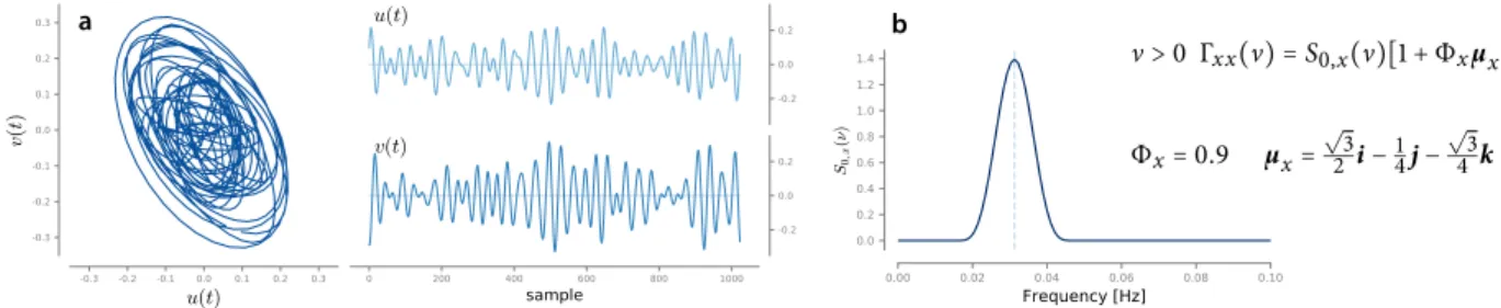
Γxx(ν), Γx y(ν) Quaternion PSD of x, quaternion cross-PSD between x and y, p.53,55

ˆΓ(p)

xx (ν), ˆΓxx(mt)(ν) periodogram and multitaper estimates of the quaternion PSD of x p.65,66

Time-frequency analysis

x+(t) Quaternion embedding of the bivariate signal x p.105

H {x} Hilbert transform of x p.106

Fgx(τ, ν) Quaternion Short-Term Fourier Transform of x using a window g p.110

Wx(τ, s) Quaternion Continuous Wavelet Transform of x p.113

WVx(τ, ν) Quaternion Wigner-Ville transform of x p.118

Acronyms

C-PSD Complementary Power Spectral Density

LTI Linear Time-Invariant

PSD Power Spectral Density

Q-CWT Quaternion Continuous Wavelet Transform

Q-STFT Quaternion Short-Term Fourier Transform

0

Introduction

In many areas of science there is the need to jointly analyze two observed real-valued signals: eastward and northward velocities of oceans currents (Gonella,1972; Thomson and Emery,2014) and winds (Hayashi,1982; Tanaka and Mandic,2007); polarized waves in optics (Brosseau,1998; Born and Wolf,

1980) and seismology (Samson,1983; Pinnegar,2006); pairs of electrode

record-ings in EEG or MEG (Sakkalis,2011; Sanei and Chambers,2013); gravitational waves (Misner, Thorne, and Wheeler,1973) and many more. Fig. 1depicts three examples of bivariate signals.

-4 -2 0 2 4 1e4 u(t) 0 500 1000 1500 2000 time[s] -4 -2 0 2 4 1e4 v(t) -4 -2 0 2 4 u(t) 1e4 -4 -2 0 2 4 v( t) 1e4 -40 -20 0 20 40 u(t) 0 50 100 150 200 250 300 350 400 time[days] -40 -20 0 20 v(t) -40 -20 0 20 40 u(t) -40 -20 0 20 40 v( t) -2 -1 0 1 2 1e-20 u(t) -7 -6 -5 -4 -3 -2 -1 0 time[s] -2 -1 0 1 2 1e-20 v(t) -2 -1 0 1 2 u(t) 1e-20 -1 0 1 v( t) 1e-20 a b c

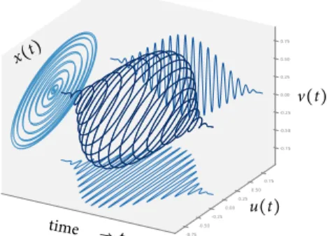
Figure 1: Three examples of bivariate signals. The time-evolution of the two components u(t) and v(t) as well as the trace in the u − v plane are represented. (a) polarized seismic wave (b) horizontal current velocities mea-sured by an oceanic drifter (c) gravitational wave polarizations emitted by a precessing coalescing binary.

A bivariate signal can be either modeled as a vector signal x∶ R → R_{or as} a complex-valued signal x∶ R → C such that

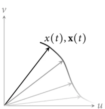
x(t) = [u(t)_v(t)] or x(t) = u(t) + iv(t) (1)

where u(t) and v(t) are real-valued signals corresponding e.g. to eastward and northward ocean current velocities. The vector and complex representations equivalently encode trajectories in the 2D plane, see Fig. 2. The choice of one over the other representation usually depends on the application area: vector-valued signals are more common in optics and geophysics. The complex

representation is more common in oceanography (Gonella, 1972; Mooers,

1973), which has popularized a decomposition of bivariate signals into counter-rotating components known as rotary components. Many recent methods developed in the signal processing literature (Schreier,2008; Lilly and Olhede,

2010a; Walden,2013; Sykulski, Olhede, and Lilly,2016) also use the complex

representation. It shall be noted that perhaps the first to recognize the potential of the complex representation to study bivariate signals were Blanc-Lapierre and Fortet (1953).

u

v

x

(t), x(t)

Figure 2: A bivariate signal defined by (1) cor-responds to a trajectory in the 2D plane.

The use of the complex representation over the vector representation has often been advocated for in the signal processing community. While this has sparked some heated debates, see for instance the discussion between Picin-bono (1996) and Johnson (1996), this choice seems to be well accepted today by the signal processing community. The often quoted advantages of the complex representation include: a preserved relation between the two real univariate components, simplified expressions, the direct availability of fundamental notions such as amplitude and phase and the geometric insights offered by complex numbers. See e.g. the recent books of Mandic and Goh (2009) and Schreier and Scharf (2010) for a detailed discussion of these advantages.

This thesis aims at providing an unifying framework for the processing of bivariate signals. For this purpose, Section0.1introduces key concepts thanks to the very first example of the monochromatic bivariate signal. Then Section0.2reviews the usual vector and complex approaches for processing bivariate signals. Section0.3presents the limitations of these two approaches and discusses the requirements that an ideal framework should satisfy. Section

0.1 A first example: the monochromatic bivariate signal

0.1.1 Vector and complex representations

A monochromatic bivariate signal is given in its vector representation by x(t) = [u(t)_{v(t)] = [}aucos(πνt+ φu)

avcos(πνt+ φv)], (2)

where au, av ≥  and φu, φv ∈ [, π) are the amplitudes and phases of the respective components. The complex representation of this signal writes

x(t) = aucos(πνt+ φu) + iavcos(πνt+ φv)

= a+eiθ+eiπνt+ a−e−iθ−e−iπνt (3)

where a+, a− ≥  and θ+, θ− ∈ [, π) are the amplitude and phase of each

phasor1_{, respectively. Eq. (3) describes the signal x(t) as a sum of two counter- 1. A phasor is here understood as a signal} of the form t↦ eiπνt_{, where ν∈ R.} rotating phasors at frequencies νand−ν. These are also called the rotary

components of the signal (Schreier and Scharf,2010).

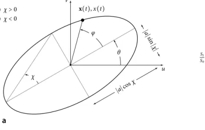
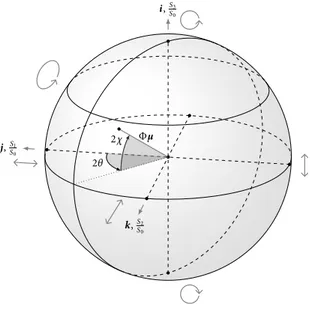
u v x(t), x(t) χ θ φ • ∣a∣cosχ ∣a∣_sin ∣χ∣ ↺ χ >  ↻ χ <  S S S S S S θ χ

a

b

Figure 3: (a) The monochromatic bivariate signal describes an elliptical trajectory in the 2-dimensional plane. (b) Poincaré sphere of polarization states. To any point on the sphere is associated a unique polarization state ei-ther described by spherical angular coordi-nates(θ, χ) or normalized Stokes parame-ters S/S, S/Sand S/S.

Fig.3a depicts the elliptical trajectory in the 2-dimensional plane defined by the monochromatic bivariate signal (2). This trajectory is described by four natural parameters. Two of them encode the geometry of the ellipse. The orientation θ ∈ [−π/, π/] gives the angle between the major axis of the ellipse and the horizontal axis. The ellipticity χ∈ [−π/, π/] characterizes the shape of the ellipse: it is directly related to the ratio between minor and major axes. For χ=  the ellipse degenerates into a line segment, while for χ = ±π/ it becomes a circle. Importantly the sign of χ gives the running direction within the ellipse: counter-clockwise if χ>  and clockwise for χ < . The two remaining parameters are classical: the amplitude a≥  controls the size of the ellipse and the phase φ ∈ [, π) gives the initial position of the signal within the ellipse.

introduction 17

0.1.2 The concept of polarization: Stokes parameters and Poincaré sphere

In optics the signal x(t) defined by (2) or x(t) defined by (3) would describe the instantaneous position of the electric field in the transverse plane, i.e. in the plane orthogonal to the direction of propagation of the light. As it describes an elliptical trajectory, the electric field is said to be elliptically polarized. Po-larization is a fundamental concept related to wave propagation, which can be found in various domains such as optics and electromagnetics (Born and Wolf,1980), seismology (Aki and Richards,2002) or gravitational wave theory (Misner, Thorne, and Wheeler,1973).

The polarization ellipse is usually described in optics by Stokes parameters. They form a set of four real-valued parameters S, S, Sand Swhich are experimentally accessible via intensity measurements. They are related to

ellipse parameters a, θ and χ like Expressions (4)–(7) correspond to the

par-ticular case where the signal is fully polar-ized. The case of partially polarized or un-polarized signals will be discussed in more detail in Chapter2.

S= a (4)

S= acos θ cos χ (5)

S= asin θ cos χ (6)

S= asin χ . (7)

The first parameter Sis purely energetic; remaining parameters S, Sand S describe the polarization state of the monochromatic bivariate signal. Being a phase term, φ does not appear in Stokes parameters.

Fig. 3b depicts the Poincaré sphere, first introduced by Poincaré (1892). This powerful geometric representation of polarization states directly connects Stokes parameters to the natural parameters a, θ and χ of the ellipse. To any point on the surface of the 2-dimensional unit sphere one associates a unique polarization state. Its spherical angular coordinates(θ, χ) give the geometric parameters of the ellipse. Its Cartesian coordinates provide the corresponding normalized Stokes parameters S/S, S/Sand S/S. The north and south pole of the Poincaré sphere describe counter clockwise and clockwise circular polarization, respectively. The equator describes linearly polarized states: the orientation θ evolves with the longitude. As one moves towards the poles, the ellipticity χ increases in absolute value and one tends to circular polarization.

0.1.3 Expressions for ellipse parameters

It is natural to search for the expression of the ellipse trajectory parameters a, θ, χ and φ in terms of the standard parameterization of each representation (vector or complex). Starting from Eq. (2) the amplitude a and phase φ read

a=√a

u+ av and φ= φu+ φ_ v . (8)

The orientation θ and ellipticity χ are given by tan θ= a_a uav

u− avcos(φu− φv) and sin χ = a uav a

u+ avsin(φu− φv) (9) when au≠ av. The case au= avcorresponds to circular polarization: it follows that χ= ±π/ and θ is undefined for this case.

The amplitude a and phase φ are obtained from the complex representation (3) as

a=√√a_{++ a}_{− and φ= θ}++ θ−

 . (10)

The orientation θ and ellipticity χ write

θ= θ+− θ_ −, and tan χ= a_a+− a−

++ a−. (11)

If one compares expressions (9) and (11) for θ and χ we see that (11) decouples the contribution from the amplitude and phases from each rotary component. This apparent simplicity is sometimes used as an argument supporting the use of the complex representation (11) over the vector representation (9), see e.g. Schreier and Scharf (2010).

0.1.4 Natural descriptors for bivariate signals

One could argue whether or not a, θ, χ and φ represent natural parameters for the elliptical trajectory depicted in Fig.3a. These parameters appear tradi-tionally in optics (Brosseau,1998; Born and Wolf,1980) thanks to the Poincaré sphere representation and the associated Stokes parameters expressions. More-over they also appeared as quantities of interest in the signal processing litera-ture, see e.g. Schreier (2008) and Walden (2013). These parameters are natural in the sense that they directly embody the joint structure of the two univariate signals that constitute the monochromatic bivariate signal. One associates a common amplitude a, a common phase φ and two geometric parameters θ and χ to the signal x(t) or x(t). This contrasts with parameterizations (au, av, φu, φv) or (a+, a−, φ+, φ−) which involve two amplitudes and two phases. In fact Eqs. (2) and (3) can be interpreted as the decomposition of the signal into, respectively, horizontal and vertical linearly polarized components and counter-clockwise and clockwise circularly polarized components. The natural or canonical parameters(a, θ, χ, φ) are very generic in the sense that they are not attached to any particular representation, i.e. to any choice of orthogonal polarizations decomposition.

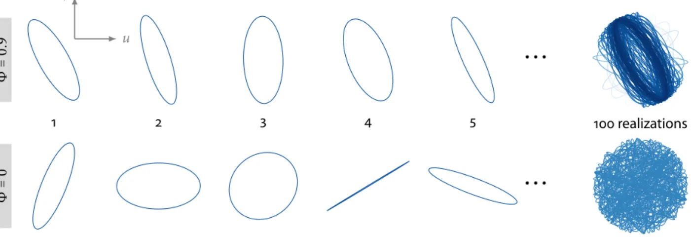
0.2 An overview of signal processing for bivariate signals

Section0.2.1and Section0.2.2first consider the case of second-order sta-tionary random bivariate signals: they form an important category of random bivariate signals whose second-order statistical properties (i.e. mean and co-variances functions) are invariant to any given time-shift. In this setting, at any given frequency the spectral contribution of the signal takes the form of a random ellipse (Walden,2013): its orientation, ellipticity, or amplitude vary over realizations. In particular we put the emphasis on the notion of (im)properness of random complex signals.

Section0.2.3and Section0.2.4then describe one of the most fundamen-tal signal processing task, i.e. linear time-invariant (LTI) filtering, in both representations.

introduction 19

Finally, Section0.2.5presents existing methods towards the characterization of instantaneous attributes of bivariate signals, and how it relates to time-frequency analysis techniques.

0.2.1 Random bivariate signals in the vector representation

For sake of simplicity, second-order stationarity is simply referred to as station-arity in what follows, and signals are assumed to be zero-mean. Consider a stationary random bivariate signal x(t) = [u(t), v(t)]⊺_{where u(t) and v(t)} are jointly stationary real-valued signals and where⊺is the transpose operator. The covariance matrix function of the vector signal x(t) is (Priestley,1981)

Rxx(τ) = E {x(t)x⊺(t − τ)} = [R_Ruu(τ) Ruv(τ)

vu(τ) Rvv(τ)] (12)

where Ruu, Rvvdenote the autocovariances of u and v, and where Ruvdenotes the cross-covariance between u and v. These are defined like

Ruu(τ) = E {u(t)u(t − τ)} , Rvv(τ) = E {v(t)v(t − τ)} , Ruv(τ) = E {u(t)v(t − τ)} . (13)

Note that Ruuand Rvv are even functions of τ, and that for all τ, Rvu(τ) = Ruv(−τ). The entry-wise Fourier transform (denoted symbolically by F) of the covariance matrix function Rxx(τ) defines the power spectral density (PSD)

matrix of x(t)

Pxx(ν) = FRxx(ν) = [P_Puu(ν) Puv(ν)

vu(ν) Pvv(ν)] , (14)

where Puu and Pvv are the PSD of u and v and where Puvis the cross-PSD between u and v. The PSD matrix Pxxis Hermitian positive semidefinite since

PSDs Puuand Pvv are real-valued nonnegative and Pvu(ν) = Puv(ν) for every ν. See e.g. Priestley (1981) for more details on spectral analysis using the vector representation.

0.2.2 Random bivariate signals in the complex representation

Complex-valued random variables and random signals have been widely stud-ied in the signal processing literature (Picinbono,1994; Amblard, Gaeta, and

Lacoume,1996a, 1996b; Picinbono and Bondon,1997; Ollila,2008; Adalı,

Schreier, and Scharf,2011). Many simulation procedures of such signals have been also proposed (Rubin-Delanchy and Walden,2007; Chandna and Walden,

2013; Sykulski and Percival,2016).

The complete statistical characterization of the second-order properties of a stationary complex signal x(t) involves two quantities: the usual autocovari-ance function Rxx(τ) and the complementary or pseudo-covariance ˜Rxx(τ). They are defined as

(autocovariance) Rxx(τ) ≜ E {x(t)x(t − τ)} , (15) (complementary-covariance) ˜Rxx(τ) ≜ E {x(t)x(t − τ)} . (16) The autocovariance function is Hermitian Rxx(−τ) = Rxx(τ) and the

com-Remark that the pseudo-covariance ˜Rxx(τ)

is simply the covariance function between x(t) and its conjugate x(t).

plementary covariance is even ˜Rxx(τ) = ˜Rxx(−τ). In the spectral domain one defines the PSD and complementary PSD (C-PSD) of the signal x as

(PSD) Pxx(ν) = FRxx(ν) , (17)

(C-PSD) ˜Pxx(ν) = F ˜Rxx(ν) . (18)

The PSD Pxx(ν) is real nonnegative but not necessarily even Pxx(−ν) ≠ Pxx(ν) as x is complex-valued. The C-PSD is complex-valued ˜Pxx(ν) ∈ C and even

˜Pxx(−ν) = ˜Pxx(ν).

Usually (Schreier and Scharf,2003b) one introduces the augmented com-plex vector signal9x(t) = [x(t), x(t)]⊺. Then the corresponding augmented covariance matrix reads

9Rxx(τ) ≜ E {9x(t)9x†(t − τ)} =⎡⎢⎢⎢ ⎢⎣ Rxx(τ) ˜Rxx(τ) ˜Rxx(τ) Rxx(τ) ⎤⎥ ⎥⎥ ⎥⎦, (19)

with† _{the conjugate-transpose operator. Its entry-wise Fourier transform} defines the augmented PSD matrix

9Pxx(ν) =⎡⎢⎢⎢ ⎢⎣ Pxx(ν) ˜Pxx(ν) ˜Pxx(ν) Pxx(−ν) ⎤⎥ ⎥⎥ ⎥⎦ . (20)

Note that the augmented PSD matrix involves expressions of the PSD at both positive and negative frequencies. The augmented PSD matrix is directly related to the PSD matrix (14) of the real vector x(t) like

9Pxx(ν) = T Pxx(ν)T† (21)

where T is defined as

T= [ i_{ −i]}. (22)

A signal x(t) is said to be second-order circular or proper if its complemen-tary covariance vanishes, i.e. ˜Rxx(τ) =  for all τ. Otherwise x(t) is said to be improper. The term proper may refer to the fact that proper complex-valued sig-nals behave very similarly to real-valued sigsig-nals (Schreier and Scharf,2003b). Equivalently, a proper signal is characterized by a null C-PSD ˜Pxx(ν) =  for all ν. Using (21), we found that a proper signal is characterized by

Puu(ν) = Pvv(ν) and Re Puv(ν) =  for all ν (23)

Or equivalently in the time-domain:

Ruu(τ) = Rvv(τ) and Ruv(−τ) = −Ruv(−τ) for all τ . (24) Stationary analytic signals without a DC component are examples of proper complex signals, see for instance Schreier and Scharf (2010, p. 57).

Remark: random ellipses The contribution of a single frequency to a station-ary random bivariate signal takes the form of a random ellipse. The statistical properties of random ellipses have been widely investigated in the signal

pro-cessing community (Walden and Medkour,2007; Rubin-Delanchy and Walden,

2008; Medkour and Walden,2008; Chandna and Walden,2011; Walden,2013).

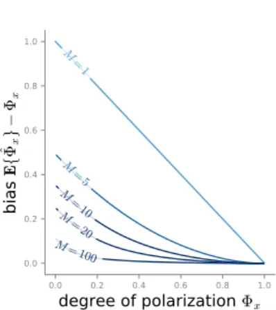
See also Barakat (1985) and Brosseau (1995) for similar results regarding the statistical properties of Stokes parameters. These results will be reviewed in Section2.4.2in our discussion on the estimation of polarization parameters.

introduction 21

0.2.3 LTI filtering in the vector representation: matrix-valued filters

Back to the vector representation of bivariate signals, consider the input x(t) and the output y(t) of an arbitrary LTI filter. Such a filter is described by its matrix impulse response m(t), a real-valued 2-by-2 matrix such that

y(t) = m ∗ x(t) (25)

where∗ denotes entry-wise convolution. If m(t) = [m(t) m(t)

m(t) m(t)] and x(t) = [x

(t)

x(t)] (26)

then the matrix-vector LTI filtering relation (25) reads explicitly y(t) = [m∗ x(t) + m∗ x(t)

m∗ x(t) + m∗ x(t)]. (27)

The filtering relation (25) can be rewritten in the frequency domain as the simple matrix-vector relation

Y(ν) = M(ν)X(ν) (28)

where Y, X and M denote entry-wise Fourier transforms of y, x and m. Note that (28) describes, for each frequency, a linear relationship between 2 dimen-sional complex-vectors. Using (28) the relationship between PSD matrices of y and x is given by

Py y(ν) = M(ν)Pxx(ν)M†(ν) . (29)

In optics, the spectral domain relation (28) is usually preferred over the time-domain relation (25). This arises since most light sources (e.g. lasers) can be assumed narrow-band; explicit frequency-dependence is often omitted. The study of linear relationships between 2 dimensional complex-vectors as in

(28) is called Jones calculus. This formalism permits to describe interactions Jones calculus is named after R. C. Jones, who introduced this formalism in a series of pa-pers published in 1941, see Jones (1941).

between polarized light and non-depolarizing linear optical systems (e.g quater-wave plates, polarizers, etc.) and is still widely used. See e.g. Gil (2007) and Gil and Ossikovski (2016) for more details.

0.2.4 LTI filtering in the complex representation: widely linear filters

The most generic LTI filter in the complex representation of bivariate signals takes the form of a widely linear filter:

y(t) = h∗ x(t) + h∗ x(t) , (30)

where h(t) and h(t) are two complex-valued impulse response functions. The signal x(t) and its conjugate x(t) are filtered separately to produce the

output signal y(t). This approach was first proposed by Brown and Crane The term ‘‘widely linear filtering‘ is due to Picinbono and Chevalier (1995).

(1969) who coined the term ‘‘conjugate linear filtering’’. Aspects regarding optimum mean-square linear estimation using such filters were developed subsequently by several authors, see Gardner (1993), Picinbono and Chevalier (1995), and Schreier and Scharf (2003b).

The widely linear filtering relation (30) can be rewritten in the augmented vector representation. Introduce the spectral domain augmented matrix of the filter as

9H(ν) ≜ [ H_H(ν) H(ν)

(−ν) H(−ν) .] (31)

The relation between augmented PSD matrices of y(t) and x(t) then is

9Py y(ν) =9H(ν)9Pxx(ν)9H†(ν) . (32)

From the augmented PSD matrix definition (20) and Eqs. (31)–(32) one sees that the filtering relation in the complex-representation involves simultane-ously positive and negative frequencies. The equivalence between the widely linear filtering relation (32) and the matrix-vector filtering relation (29) is readily obtained using transformation (21).

0.2.5 Instantaneous ellipses and time-frequency analysis

In practical situations where a narrowband bivariate signal is acquired, the signal trajectory will in general take the form of a time-varying ellipse. Instan-taneous ellipse parameters then characterize the nonstationary behavior of the signal. For deterministic signals, Lilly and Gascard (2006) have proposed the modulated elliptical signal model in the complex representation

x(t) = eiθ(t)_{[c(t) cos φ(t) + id(t) sin φ(t)] (33)}

where c(t) ≥  and where d(t) can take any sign. The angle θ(t) ∈ [−π/, π/] encodes the instantaneous orientation of the ellipse; φ(t) ∈ (−π, π) gives the instantaneous phase, i.e. the instantaneous position of x(t) around the ellipse. Quantities c(t) and ∣d(t)∣ describe the instantaneous major and minor axes of the ellipse, respectively. The sign of d(t) reflects the direction of circulation around the ellipse. As shown by Lilly and Olhede (2010a), these instantaneous parameters can be obtained from pairs of analytic signals: either from the analytic signal of the vector[u(t), v(t)] or from the analytic signal of the complex augmented vector[x(t), x(t)].

For the characterization of generic, i.e. wideband, nonstationary bivariate signals various methods have been proposed. For the nonstationary random case (Hindberg and Hanssen,2007; Schreier,2008), it consists in examining suitable correlations or coherences using pairs of time-frequency represen-tations of complex-valued signals. Alternative approaches using the vector representation have been proposed in the deterministic case, mainly by the geophysics community (Diallo et al.,2005; Roueff, Chanussot, and Mars,2006; Pinnegar,2006). We also note that bivariate extensions (Rilling et al.,2007;

Tanaka and Mandic,2007) of the empirical mode decomposition (EMD)

introduction 23

0.3 An ideal framework for bivariate signal processing?

0.3.1 Limitations of existing methods

Existing approaches are based on the use of either the vector x= [u(t), v(t)]⊺ or complex x(t) = u(t) + iv(t) representation of bivariate signals. Such approaches exhibit intrinsic limitations which prevent to consider them as an ideal framework for processing bivariate signals. Below we detail point-by-point these limitations.

No direct description in terms of natural ellipse parameters As already dis-cussed in Section0.1for the simple monochromatic bivariate case, neither the vector nor complex representation permits a direct description of bivariate signals in terms of natural elliptical trajectory parameters a, θ, χ and φ. This issue propagates to even more challenging scenarios, e.g. non-stationary or random signals. Parameters must be determined from pairs of amplitude-phase quantities, a procedure which implicitly implies a decomposition of the bivariate signal into a peculiar orthogonal polarizations basis. In the vector representation, natural ellipse parameters are obtained from the amplitude and phase of the linear horizontal(au, φu) and linear vertical polarization (av, φv). The complex representation yields amplitude and phase of circularly polarized components, counter-clockwise (a+, φ+) and clockwise (a−, φ−).

An ideal framework should feature this direct description in terms of nat-ural ellipse parameters, in order not to be subject to a particular orthogonal polarizations decomposition. This would provide straightforward interpreta-tions and greatly simplify the synthesis of bivariate signals with prescribed physical properties.

Interpretability of positive frequencies only in the complex representation For This issue is specific to the complex represen-tation of bivariate signals. The Fourier trans-form of the vector signal x(t) exhibits Her-mitian symmetry and one can consider only positive frequencies Fourier vectors.

a physicist it is natural to consider positive frequencies only as, per definition, frequency is the number of oscillations per time unit (Cohen,1995). For real-valued signals this can be mathematically justified thanks to the Hermitian symmetry X(−ν) = X(ν) of their Fourier transform: ‘‘negative frequencies’’ do not convey any supplementary information to positive ones. This authorizes useful identifications, e.g. between the cosine model cos(πνt) and the com-plex exponential exp(iπνt). It also enables the construction of the analytic signal of a real signal (Gabor,1946; Ville,1948), which is the foundation for time-frequency analysis (Flandrin,1998).

To that extent, the complex representation of bivariate signals is not satisfac-tory as both positive and negative frequencies have to be considered: the Fourier transform of a complex signal x(t) no longer satisfies Hermitian symmetry. Negative frequencies are associated to clockwise rotating components and pos-itive frequencies are attached to counter-clockwise rotating components. This refers to the so-called rotary spectrum analysis popularized by oceanographers (Gonella,1972). At a given (physical) frequency∣ν∣ the circulation direction in the ellipse is recovered by comparing amplitudes at−ν and ν, see Eq. (11).

An ideal framework using the complex representation of bivariate signals should feature a nice correspondence between mathematical (positive and negative) and physical (positive only) frequencies. This would allow natural

interpretations of the spectral content of bivariate signals.

Physical interpretations of (im)properness The notion of (im)properness of complex-valued variables and signals has been of fundamental importance in the signal processing literature: see e.g. Adalı, Schreier, and Scharf (2011) for a review. Impropriety surely is meaningful when considering complex signals created from real (univariate) signals, e.g. analytic signals or complex baseband representation of real signals. It is particularly useful in communications, where impropriety arises from in-phase/quadrature imbalance due to receiver or channel imperfections, or when the transmitted signal is non-stationary2.

2. Analytic signals of nonstationary ran-dom real signals are known to be improper (Picinbono and Bondon,1997; Schreier and Scharf,2003a).

Many works (see e.g. Schreier and Scharf (2010) for a review) have shown that taking into account impropriety of complex signals increases performances of detection and estimation algorithms.

However one could question the physical relevance of this notion for (ran-dom) bivariate signals, i.e. for signals such as polarized waves, surface wind or ocean currents measurements.

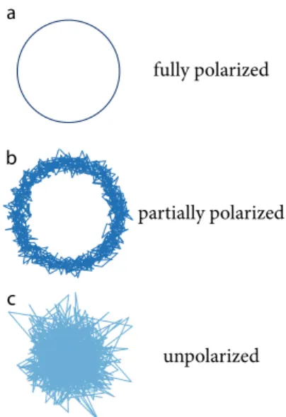
a b c fully polarized partially polarized unpolarized

Figure 4: Three proper complex signals with very different polarization properties. (a) a fully circularly polarized monochromatic sig-nal with frequency ν. (b) signal in (a)

cor-rupted by additive proper white Gaussian noise. The signal is partially polarized at fre-quency ν(c) proper white Gaussian noise is

unpolarized.

Fig.4supports our discussion by depicting three proper signals which how-ever carry very different physical properties. Fig.4a represents a monochro-matic bivariate signal with frequency νthat is fully circularly polarized. Fig.

4b displays this signal corrupted by additive proper white Gaussian noise. The signal is then said to be partially polarized at frequency ν. Fig. 4c shows a realization of proper white Gaussian noise, which corresponds to an un-polarized signal (at all frequencies.) As these three examples demonstrate, (im)properness seems not to be the most relevant feature when dealing with physical properties, e.g. polarization, of bivariate signals.

In our opinion an ideal framework should provide a direct description of bivariate signals in terms of relevant physical parameters. This should provide a straightforward classification or discrimination of bivariate signals based on physically interpretable properties, such as the degree of polarization.

Interpretation of LTI filtering relations A common limitation of both the vec-tor and complex representation is the lack of direct interpretability of filtering relations (25) and (30). Similar issues arise with relations between PSDs (29) and (32). For the univariate case, filters are described in the spectral domain by the usual filtering relation

Y(ν) = G(ν)X(ν) (34)

where G(ν) is frequency response of the filter. Its magnitude ∣G(ν)∣ and phase arg G(ν) have a natural interpretation in terms of gain and phase delay of the filter, respectively. Such physical interpretations are lacking in the bivariate case, as shown by LTI filtering expressions in the vector (25) and complex (30) representations.

A ideal framework must be able to provide such interpretations. It will improve the ability to specify desired behavior of filters for bivariate signals, and to tailor their use to the physical properties of bivariate signals.

Systematic time-frequency analysis A comprehensive and generic time-frequency analysis theory for bivariate signals does not exist in the vector setting, neither

introduction 25

representation does the complex representation. As already mentioned, exist-ing approaches rely on the simultaneous processexist-ing of pairs of time-frequency representations (Hindberg and Hanssen,2007; Schreier,2008; Roueff, Chanus-sot, and Mars,2006; Diallo et al.,2005) Data-driven methods such as bivariate

extensions of the EMD (Rilling et al.,2007; Tanaka and Mandic,2007) have Note that by spectrogram we mean a quadratic or bilinear time-frequency representation based on a short-term Fourier transform.

also been proposed. However, fundamental notions such as the spectrogram of a bivariate signal are not yet defined.

One foundation for the time-frequency analysis of bivariate signals was described by Lilly and Gascard (2006) and Lilly and Olhede (2010a) with the modulated ellipse model (33). However as pointed out by the authors in Lilly and Olhede (2010a) this model is not able to separate multicomponent bivariate signals, as it is based on pairs of analytic signals. It may also appear that the modulated ellipse model (33) is somehow arbitrary and not completely theoretically grounded.

An ideal framework should provide meaningful and physically interpretable time-frequency representations for bivariate signals. Those should encompass and extend well-known concepts from usual time-frequency analysis such as analytic signals, spectrograms, scalograms as well as generic (i.e. bilinear) time-frequency representations.

0.3.2 Summary of requirements

To summarize, an ideal and complete framework for processing bivariate signals should exhibit three distinctive and equally important features: ▸ straightforward physical descriptions: usual quantities from signal processing

e.g. power spectral densities, LTI filters or time-frequency representations should be defined directly in terms of meaningful physical parameters. In addition, the framework should feature a desirable correspondence between negative and positive frequencies. These properties would allow direct interpretations and greatly simplify the design of many standard operations, such as filtering.

▸ mathematical guarantees: the approach should gather all necessary and desirable mathematical properties such as the conservation of energetic quantities or the inversion of time-frequency representations.

▸ computationally fast implementations: the proposed framework should come with tools that are as numerically efficient as existing approaches. The last two requirements are crucial factors: the physical interpretability of the framework must preserve mathematical properties and numerical efficiency. Fulfilling these three requirements from, respectively, physics, mathematics and computer science would make the proposed approach a true signal pro-cessing framework (Flandrin,2018).

0.4 Contributions and outline

This thesis provides an unifying framework for the processing of bivariate signals. The proposed approach addresses all aforementioned limitations of existing approaches. It relies on two key ingredients. First, just like real-valued or univariate signals are usually embedded in complex numbers for ease of study, we embed bivariate signals – seen as complex-valued signals – in their

natural extension, the set of quaternionsH. Second the definition of a dedicated quaternion Fourier transform offers a meaningful spectral representation to bivariate signals. Thus the approach yields elegant, compact and efficient computations. Physical parameters describing the polarization properties of bivariate signals are naturally embedded in the proposed framework. It enables straightforward generalizations of usual signal processing notions such as spectral densities, filters, analytic signals or spectrograms to the bivariate case.

The proposed framework sheds light upon the physics of bivariate signals. More importantly, it does not sacrifice any fundamental mathematical guaran-tees nor computationally fast implementations. Any new quantity introduced within the proposed framework is validated by a theorem or a proposition.

A companion open-source Python package called BiSPy3implements our 3. BiSPy: Bivariate Signal Processing in

Python.

Documentation, tutorials and code at É bispy.readthedocs.io/ ‡ github.com/jflamant/bispy

findings for the sake of reproducible research.

The potential of quaternion algebra and its relatives – such as Pauli matrices – has been recognized for long time in optics (Richartz and Hsü,1949; Marathay,

1965; Whitney,1971; Pellat-finet,1984). This stems from its ability to give an

insightful geometric treatment of polarization states. Many works, recently reviewed by Tudor (2010a,2010b), have taken advantage of this fact to provide a pure operatorial, ‘‘matrix-free’’ formalism for the geometric description of polarization states and their interaction with linear (optical) systems. In fact this potential was even recognized long time ago by Hamilton (1844), the inventor of quaternions, in a letter to his friend Graves (17th_{October, 1843)}

å There seems to me to be something analogous to polarized intensity in the pure imaginary part; and to unpolarized energy (indifferent to direction) in the real part of a quaternion: and thus we have some slight glimpse of a future Calculus of Polarities. æ

As pointed out by Karlsson and Petersson (2004), if Hamilton had developed such ‘‘calculus of Polarities’’ he would have

pre-ceded Jones (1941) and Mueller (1943) by al-most a century.

As we shall see in Chapter2, Hamilton’s prediction was almost correct: the only difference is that the real part of the quaternion power spectral density contains the sum of contributions from the unpolarized and polarized parts of the signal, respectively.

However we note that existing results are not directly applicable to the case of bivariate signals. Relations presented by Tudor (2010a,2010b) and refer-ences therein are only given at the power spectral density level. Global phase effects are omitted and no direct or practical filtering relations are available. In addition as it focuses mainly on the monochromatic case, the formalism lacks a nice time-frequency duality which would make easy the handling of generic wideband bivariate signals.

Le Bihan, Sangwine, and Ell (2014) made a first step towards handling bi-variate signals (seen as complex numbers) with a quaternion Fourier transform. They studied some of its properties and defined a bivariate analogue to the analytic signal, a key step towards the time-frequency analysis of bivariate sig-nals. Unfortunately, the physical interpretation of their approach was limited to specific cases and thus lacked generality. Nonetheless these preliminary results form the starting point of this thesis.

This manuscript is divided into 5 chapters that describe the systematic construction of a complete framework for the processing of bivariate signals.

introduction 27

At the end of each chapter, appendices gather related complementary results and proofs.

Chapter1introduces the two ingredients of the proposed framework: quater-nion algebra and the quaterquater-nion Fourier transform (QFT). In particular the properties of the QFT are studied in detail. We provide new results show-ing that the QFT is a well-defined mathematical object similar to the usual Fourier transform. We notably demonstrate a generalized Parseval-Plancherel theorem, which reveals that the QFT not only preserves energy but also an-other quadratic geometry-related quantity. The end of this chapter settles our framework for the processing of bivariate signals. The use of the QFT makes it possible to give a meaningful and physically interpretable quaternion-valued spectral representation of bivariate signals seen as complex-valued signals. The material presented in this chapter has been published in an international journal (Flamant, Le Bihan, and Chainais,2017e).

Chapter 2discusses the spectral analysis of bivariate signals. It focuses mainly on the case of second-order stationary random bivariate signals. We prove a spectral representation theorem for harmonizable signals. This key result introduces the quaternion power spectral density (PSD) of a bivariate signal. Another key quantity, the quaternion autocovariance of a bivariate signal, is defined thanks to a Wiener-Khintchine-like theorem for the QFT. The quaternion PSD has a direct interpretation in terms of polarization features, namely frequency-dependent Stokes parameters. We also discuss the role of the degree of polarization, a natural parameter which quantifies the dispersion of the polarization ellipse at each frequency. Nonparametric spectral estima-tion is investigated in detail and we show that the estimaestima-tion of polarizaestima-tion quantities requires special care. Numerical experiments and illustrative exam-ples support our findings. This chapter includes material from publications in an international journal (Flamant, Le Bihan, and Chainais,2017c) and a contribution to the national conference GRETSI 2017 (Flamant, Le Bihan, and Chainais,2017a).

Chapter3deals with the theory of linear time-invariant (LTI) filtering for bivariate signals. Based on an usual decomposition from polarization optics, we decompose LTI filters into unitary and Hermitian ones. Each class has natural interpretation in terms of fundamental properties of optical media: unitary filters model birefringence whereas Hermitian filters model diatten-uation effects. The proposed framework directly gives filtering relations in terms of the eigenvalues and eigenvectors of the filter. It reveals the physical specificity of each filter and makes it easy to prescribe or design filters for bi-variate signals. We demonstrate the relevance of the approach on two standard tasks of signal processing: spectral synthesis of stationary Gaussian signals and Wiener filtering. It also yields original decompositions of bivariate signals in two parts with prescribed properties. These promising results have been accepted for publication in an international journal (Flamant, Chainais, and Le Bihan,2018a). They were also presented at the international conference SSP 2018 (Flamant, Chainais, and Le Bihan,2018b) where we received a Best Student paper award.

Chapter4addresses the time-frequency analysis of bivariate signals. We define a bivariate analogue of the analytic signal called the quaternion embed-ding of a complex signal. It allows for direct identification of instantaneous amplitude and phase, as well as instantaneous polarization attributes. We introduce the short-term quaternion Fourier transform and quaternion contin-uous wavelet transform to overcome the inherent limitations of the quaternion embedding. Their properties are studied in detail. Two fundamental theorems guarantee their inversion. They also ensure the interpretability of associated time-frequency-polarization representations, namely polarization spectrogram and polarization scalogram, respectively. An asymptotic analysis ensures that these time-frequency-polarization representations localize meaningfully. The last part of this chapter develops a generic approach to the construction of time-frequency-polarization representation. We define the quaternion Wigner-Ville distribution and provide a construction of the Cohen class of bilinear representations. Numerical experiments from simulated and real-world data support our analysis. The majority of these results has been published in an international journal (Flamant, Le Bihan, and Chainais,2017e). It was pre-sented at the international conference ICASSP 2017 (Flamant, Le Bihan, and Chainais,2017b) and at the national conference GRETSI 2017 (Flamant, Le Bihan, and Chainais,2017d).

Chapter5explores the potential of the framework for the characterization of the polarization pattern of gravitational waves (GW) emitted by precessing binaries. This work results from a collaboration with Eric Chassande-Mottin and Fangchen Feng. Precession of emitting GW sources induces a modulation of the polarization pattern of the GW. We show that the framework developed in this thesis grants a new nonparametric characterization method for these effects. Importantly the approach does not assume any dynamical model for precession. Hence it is very promising for the future of GW characterization as it has the potential of revealing any dynamical effect that affects the GW polarization pattern. Our findings are illustrated on simulated data in noise-free and in realistic simulated noise contexts. These results have been presented at the international conference EUSIPCO 2018 (Flamant et al.,2018).

The concluding chapter, page145, presents conclusions and discusses

some of the prospects triggered by the work presented in this manuscript. The appendix, page169describes the main results from a collaboration with Rémi Bardenet and Pierre Chainais. This joint work was performed in parallel with the research framework for bivariate signals developed in this thesis. We have studied the distribution of the zeros of the spectrogram of white Gaussian noise when the window is itself Gaussian. Our contributions are threefold: we rigorously define the zeros of the spectrogram of continuous white Gaussian noise, we explicitly characterize their statistical distribution, and we investigate the computational and statistical underpinnings of the practical implemen-tation of signal detection based on the statistics of spectrogram zeros. This appendix reproduces the article “On the zeros of the spectrogram of white noise,” Bardenet, Flamant, and Chainais (2018), currently under review at Applied and Computational Harmonic Analysis.

introduction 29

List of publications

International journals

N _{J. Flamant, P. Chainais, and N. Le Bihan. 2018a. “A complete framework for}

linear filtering of bivariate signals.” IEEE Transactions on Signal Processing 66, no. 17 (September): 4541–4552. doi:10.1109/TSP.2018.2855659

N _{J. Flamant, N. Le Bihan, and P. Chainais. 2017c. “Spectral analysis of}

station-ary random bivariate signals.” IEEE Transactions on Signal Processing 65 (23): 6135–6145. doi:10.1109/TSP.2017.2736494

N _{J. Flamant, N. Le Bihan, and P. Chainais. 2017e. “Time-frequency analysis of}

bivariate signals.” In Press, Applied and Computational Harmonic Analysis. doi:10.1016/j.acha.2017.05.007

N _{R. Bardenet, J. Flamant, and P. Chainais. 2018. “On the zeros of the}

spec-trogram of white noise.” manuscript accepted for publication in Applied and Computational Harmonic Analysis. eprint:arXiv:1708.00082

International peer-reviewed conferences

 _{J. Flamant, P. Chainais, E. Chassande-Mottin, F. Feng, and N. Le Bihan. 2018.}

“Non-parametric characterization of gravitational-wave polarizations.” In 26th European Signal Processing Conference (EUSIPCO), 2018, 1–5. September

 _{J. Flamant, P. Chainais, and N. Le Bihan. 2018b. “Linear filtering of bivariate}

signals using quaternions.” In IEEE Statistical Signal Processing Workshop (SSP), 2018, Freiburg, 1–5. Best Student Paper Award

 _{J. Flamant, N. Le Bihan, and P. Chainais. 2017b. “Polarization spectrogram}

of bivariate signals.” In IEEE International Conference on Acoustics, Speech, and Signal Processing (ICASSP), 2017, New Orleans, USA

National peer-reviewed conferences

 _{J. Flamant, N. Le Bihan, and P. Chainais. 2017a. “Analyse spectrale des}

sig-naux aléatoires bivariés.” In GRETSI 2017. Juan-les-Pins, France

 _{J. Flamant, N. Le Bihan, and P. Chainais. 2017d. “Spectrogramme de}

polari-sation pour l’analyse des signaux bivariés.” In GRETSI 2017. Juan-les-Pins, France

1

Quaternion Fourier transform

for bivariate signals

The purpose of this chapter is to lay the foundations of the proposed framework Chapter contents

1.1 Quaternions 32

Definition•Quaternion operations

•Complex subfields•Polar forms•

Quaternions and 3D rotations•

1.2 Quaternion Fourier transform 35

Definition, existence, inversion •

Properties of the Quaternion Fourier transform•

1.3 Processing bivariate signals

with the quaternion Fourier

transform 39

Bivariate signals•Choice of the axis of the QFT•Monochromatic bivariate signals•

1.4 Conclusion 42

Appendices

1.A Euler polar form computation 44

1.B Hilbert spaces over quaternions 44

1.C Discretization of the quaternion

Fourier transform 45

Discrete-time quaternion Fourier transform • Discrete quaternion Fourier transform•

1.D Proofs of quaternion Fourier

transform properties 46

Convolution properties (1.34)

and (1.35) • Theorem 1.1 (Parseval-Plancherel) • Theorem 1.2 (Gabor-Heisenberg uncertainty principle)• for the analysis and filtering of bivariate signals. This framework relies on two

key ingredients: quaternions and the quaternion Fourier transform. We will first take a step back to gather the mathematical properties of these two elements in a generic setting. Then we will show that quaternions and the quaternion Fourier transform provide a natural embedding for bivariate signals viewed as complex-valued signals. The overall approach can be compared to the case of real-valued or univariate signals: these are usually embedded in the complex domain thanks to the Fourier transform, leading to many quantities of interest such as amplitude and phase. Here the fruitful combination of quaternions and quaternion Fourier transform yields an efficient, rigorous and easily interpretable framework for the handling of bivariate signals.

Quaternions form a four-dimensional algebra. A quaternion-valued signal can thus convey up to four channels simultaneously, giving rise to many signal processing applications. Examples include three-channel signal processing in geophysics (Le Bihan and Mars,2004; Miron, Le Bihan, and Mars,2006; Rehman and Mandic,2010) and more generic four-channel signal processing (Took and Mandic,2009,2010; Vía, Ramírez, and Santamaría,2010). Quater-nions also appear in the representation of the monogenic signal (Felsberg and Sommer,2001; Clausel, Oberlin, and Perrier,2015), which is an extension of the analytic signal to the case of (bi-dimensional) images. In contrast to these existing approaches, quaternions are used in this manuscript as a natural embedding for bivariate signals viewed as complex-valued signals.

The name quaternion Fourier transform does not refer to a single mathe-matical instance. The set of quaternions exhibits two additional dimensions compared to the usual complex field thus providing a large choice of quaternion Fourier transform definitions. Motivated by applications in image processing

(Sangwine,1996; Ell and Sangwine,2007; Bülow and Sommer,2001), most Quaternion Fourier transforms have been widely used in color image processing, since RGB information can be stored in the vector part (imaginary part) of a quaternion, see Ell, Le Bihan, and Sangwine (2014) and references therein.

definitions concern signals x ∶ R _{→ H, i.e. two-dimensional quaternion} Fourier transforms. See e.g. Hitzer (2007) for possible definitions and their resulting properties. In general, two-dimensional quaternion Fourier trans-forms lack some usual properties of the complex Fourier transform, which may have hampered their widespread use. In contrast we study here the generic one-dimensional quaternion Fourier transform first introduced by Jamison (1970) in his PhD dissertation. This quaternion Fourier transform exhibits properties similar to the usual complex Fourier transform and enjoys a numer-ically efficient implementation relying on FFTs only. We demonstrate that the quaternion Fourier transform builds a solid ground for the representation and analysis of bivariate signals by a suitable choice of its free-parameter, its axis.

The formal construction of the proposed framework has been published in an international journal (Flamant, Le Bihan, and Chainais,2017e):

N _{J. Flamant, N. Le Bihan, and P. Chainais. 2017e. “Time-frequency analysis of}

bivariate signals.” In Press, Applied and Computational Harmonic Analysis. doi:10.1016/j.acha.2017.05.007

In this paper we reviewed some known properties of the quaternion Fourier transform and proved some additional ones, including the generalized Parseval-Plancherel Theorem1.1and the Gabor uncertainty principle (Theorem1.2). This paper also discusses the choice of the axis of the quaternion Fourier transform to efficiently process bivariate signals, as well as the use of a specific quaternion polar form to build meaningful interpretations.

First, we review quaternion algebra in Section1.1. Then Section1.2studies the generic mathematical properties of the quaternion Fourier transform. Section1.3combines these two elements to establish a meaningful framework for the spectral description of bivariate signals. Appendices1.Ato1.Cgather complementary elements. Proofs of the main properties of the quaternion Fourier transform are collected in Appendix1.D.

1.1 Quaternions

In this section we only cover the necessary material on quaternions for this manuscript and refer to dedicated textbooks for more details. References include the original work of Hamilton (1866) and more recent textbooks such as Ward (1997) and Conway and Smith (2003). Historical aspects can be found in Crowe (1967) and Baez (2002). See also Ell (2013) for a recent review on the use of quaternions in signal processing.

Quaternions were first described by Sir William Rowan Hamilton in 1843. We recommend the musical video of A Capella Science (2016) for a narrative of Hamilton’s life and achievements.

Hamilton had understood the tight link between complex numbers and 2-dimensional geometry and has thus tried for many years to find the corre-sponding algebra to handle 3-dimensional geometry. His quest for a system of

algebraic triplets however failed until he discovered on the 16th_{of October 1843 Even his children asked him ‘‘Well, Papa, can}

you multiply triplets?’’, to which he answered ‘‘No, I can only add and substract them’’.

that he needed a fourth dimension to handle them, leading to the quaternions. He immediately carved the rule for quaternion multiplication into the stone of the Brougham bridge in Dublin. This carving has now disappeared and has been replaced by a plaque honoring his discovery. Hamilton devoted his last 20 years to the study of his quaternions which culminated in his book, Elements of quaternions. After his death in 1865 quaternions remained fashionable for some time, but they were rapidly superseded by the advent of modern vector calculus through the work of Gibbs and Heaviside. Since the end of the 20th century, quaternions have however regained some attention primarily due to their ability to efficiently represent 3D rotations. They are used in numerous applications, ranging from computer graphics to robotics.

1.1.1 Definition

The set of quaternions is denoted byH in honor of Hamilton. Quaternions form a four-dimensional noncommutative division ring over the real numbers. Any quaternion q∈ H reads in its Cartesian form

quaternion fourier transform for bivariate signals 33

where a, b, c, d ∈ R are its components. Imaginary units i, j, k satisfy the fundamental formula for quaternion multiplication

i_{= j}_{= k}_{= i jk = − (1.2)}

from which one deduces

i j= −ji = k jk= −k j = i ki= −ik = j.

(1.3) These cyclic relations (1.3) highlight the noncommutative nature of quaternion multiplication, i.e. for q, q′∈ H in general qq′_{≠ q}′_{q. However usual operations} such as addition, scalar multiplication and equality behave similarly to the complex case. Let q= a + bi + c j + dk and q′_{= a}′_{+ b}′_{i+ c}′_{j+ d}′_{k denote two} quaternions, one has

(addition) q+ q′_{= q}′_{+ q = (a + a}′_{) + (b + b}′_{)i + (c + c}′_{)j + (d + d}′_)k (scalar multiplication) ∀λ ∈ R, λq = qλ = λa + λbi + λc j + λdk

(equality) q= q′_{⇔ a = a}′_{, b= b}′_{, c= c}′_{, d= d}′_. Any quaternion q∈ H can be decomposed into its scalar part S(q) and its vector partV(q) such that

q= S(q) + V(q), (1.4)

where

S(q) = a V(q) = bi + c j + dk, (1.5)

The scalar part is real-valuedS(q) ∈ R, whereas the vector part V(q) ∈ S(q) and V(q) are also called the real and imaginary parts of q. When S(q) = , q is called a pure quaternion.

span{i, j, k} is purely imaginary . This vector part V(q) can be uniquely identified to a vector ofR_.

The product of two quaternions q, q′ ∈ H reads using the scalar-vector decomposition

qq′_{= S(q)S(q}′_{) − ⟨V(q), V(q}′_{)⟩ + S(q)V(q}′_{) + S(q}′_{)V(q) + V(q) × V(q}′_{) (1.6)}

where⟨⋅, ⋅⟩ and ⋅ × ⋅ denote the usual inner product and cross product of R_. Eq. (1.6) emphasizes the noncommutative nature of the quaternion product, since the cross-productV(q) × V(q′_{) is noncommutative.}

1.1.2 Quaternion operations

The quaternion conjugate of q is denoted by q and is obtained by reversing the sign of its vector part

q= S(q) − V(q) = a − bi − c j − dk. (1.7)

Importantly the order of the quaternion product is flipped by conjugation, i.e. for q, q′∈ H one has

qq′_{= q}′_{q. (1.8)}

The modulus of a quaternion q∈ H is When∣q∣ = , q is called a unit quaternion.