Describing Functions for Information Channels Subject to
Packet Loss and Quantization
MASSACHUSES 1-rN fTEOF TECHNOLOGY
by
OCT
16 2014
Eric Gilbertson
LIBRARIES
S.B.,
Massachusetts Institute of Technology (2008)
S.M., Massachusetts Institute of Technology (2010)
Submitted to the Department of Mechanical Engineering
in partial fulfillment of the requirements for the degree of
Doctor of Philosophy
at the
MASSACHUSETTS INSTITUTE OF TECHNOLOGY
September 2014
@
Massachusetts Institute of Technology 2014. All rights reserved.
Signature redacted
A uthor ... ...
Department of Mechanical Engineering
August 1, 2014
Signature redacted
Certified by ...
...
Franz S. Hover
Finmeccanica Career Development Professor of Engineering
Thesis Supervisor
Signature redacted
Accepted by...David
.
t
David E. Hardt
Chairman, Department Committee on Graduate StudentsDescribing Functions for Information Channels Subject to Packet Loss
and Quantization
by
Eric Gilbertson
Submitted to the Department of Mechanical Engineering on August 1, 2014, in partial fulfillment of the
requirements for the degree of Doctor of Philosophy
Abstract
Wirelessly connected robotic systems have become widespread in the terrestrial, aerial and underwater environments. Examples include autonomous underwater vehicle (AUV) coor-dination and navigation, Wide Area Measurement System (WAMS) control of power grids, and automobile networked subsystems control. As one would expect, demand on through-put grows to fill the available channel capacity; in a clean short-range RF setting, entire images may be transferred in each cycle, as part of a vision-based control system, whereas in the ocean, acoustic channels with perhaps twenty bits per second allow only the most basic sensor and command information to be shared regularly. Packet-based wireless com-munication systems like these that operate near their limits are necessarily quantized, and often prone to loss. These properties directly impact the overall system performance, and thus methodologies for understanding and designing feedback systems with quantization and packet loss are valuable. This thesis makes several contributions to feedback control of systems subject to quantization and stochastic packet loss in the sensor feedback channel.
First, we derive and verify describing functions (DFs) for information channels sub-ject to quantization and packet loss. The DFs represent the loss and quantization effects by frequency- and amplitude-dependent gains and phases, similar to transfer functions. These DFs are unique because, unlike most other DFs that describe hardware and physical elements, these describe stochastic information channels. DFs are presented for a general codec algorithm, and for four commonly-used sensor-feedback codecs: Zero-Output, Hold-Output, Linear Filter, and Modified Information Filter. These are each given as closed-form mathematical expressions of the provably optimal gains and phases for each case, with each decoder a specific case of the general codec algorithm. Gains and phases predicted by the models are verified by simulation for open-loop stable, open-loop unstable, minimum phase and nonminimum phase example systems.
Second, we show how the DFs can be used as analysis tools to predict limit cycles in dynamic feedback control systems. Computation times using the DFs are shown to be orders of magnitude faster than those from simulation for these calculations.
Third, we propose a synthesis method to use the DFs to design a codec for the sensor feedback channel that decreases limit cycle amplitudes induced by quantization and packet
loss for a large class of systems. Up to three-fold reductions in limit cycle amplitudes
are shown, with the tradeoff being slightly higher system sensitivity to disturbances and slightly higher steady state errors to step inputs. The designed codec is of the special and simple form of a constant times the sent signal if the signal is received and a different constant times the previous decoded signal if the sent signal is lost. This is the equivalent structure and computation complexity to both Zero-Output and Hold-Output decoders. A DF for this decoder allows the constants to be solved for as functions of target limit cycle amplitudes. The constants reduce to solutions of cubic equations, which are guaranteed to have a real root, and thus the codec is physically realizable. The codec allows for multiple limit cycle frequency solutions for the same amplitude solution. The analysis and synthesis tools are verified both by numerical examples, and by a physical experiment controlling heading of a small robotic raft where the designed decoder results in smaller limit cycles than does a linear-filter-based decoder.
Thesis Supervisor: Franz S. Hover
Acknowledgments
I would first like to thank my advisor Professor Franz Hover and my committee members Professor Hardt and Professor Leonard for all their guidance on the project. Thank you to my labmates Brooks, Chris, Josh, Mei, and Pedro for helping with the kayak experiments in the river, with the raft experiments in the pool, and helping me with questions during lab lunch presentations. Thanks also to my brother Matthew for helping me debug problems, often in talks as we ran around the Charles River or hiked up a mountain. I'm also grateful to the MIT Outing Club for getting me up in the mountains for breaks from schoolwork.
This work is supported by the Office of Naval Research, Grant N00014-09-1-0700, the National Science Foundation, Contract CNS-1212597, Chevron Energy Technology Company, and Finmeccanica.
This doctoral thesis has been examined by a Committee of the Department
of Mechanical Engineering as follows:
Professor Franz Hover...
Chairman, Thesis Committee
Associate Professor
Professor D ave Hardt...
Member, Thesis Committee
Professor of Mechanical Engineering
Professor John Leonard ...
.... ...o .Member, Thesis Committee
Professor of Mechanical Engineering
Contents
1 Introduction 23
1.1 Motivation and Problem Statement . . . 23
1.1.1 Underwater Applications . . . 24
1.1.2 Terrestrial Applications . . . 26
1.2 Overview and Contributions of the Thesis . . . 27
1.3 Assumptions . . . 30
1.4 Example Systems Studied. . . . .. 30
1.5 Summary . . . 31
2 Background 33 2.1 Introduction . . . 33
2.2 Control with Quantization . . . 33
2.3 Control with Packet Loss . . . 35
2.4 Control with Quantization and Packet Loss . . . 37
2.5 Limit Cycles . . . 38
2.6 Control of Underwater Thrusters . . . 39
2.6.1 Thruster Modeling . . . 39
2.6.2 Thruster Control . . . 40
2.7 Synopsis of Literature Review . . . 41
2.8 Summary . . . .. 42
3 Experiments with Packet-Loss Robust Control 45 3.1 Introduction . . . 45
3.2 3.3 3.4 3.5 3.6 3.7
Hardware and Operating Environment . . . . System Model . . . . ... .. MIF Experimental Setup . . . . Physical Connectivity . . . . Experimental Results . . . ..
Summary . . . .
4 Describing Function Derivations
4.1 Introduction . . . . 4.2 Describing Function for General Multiple Input Multiple Output
Informa-45 47 48 48 50 51 53 53
tion Channels Subject to Packet Loss . . . . 4.3 Describing Functions for Spec
4.3.1 Loss with Zero-Output 4.3.2
4.3.3 4.3.4
Loss with Hold-Outpu Loss with LQG-Type Loss with Modified In 4.4 Model Verification . . . . . 4.4.1 Convergence . . . . 4.4.2 LH Verification . . . 4.4.3 LF Verification . . . 4.4.4 LM Verification . . . 4.4.5 Coupled Losses . . .
4.5 Quantizer Describing Functio
4.5.1 Uniform Quantizer
4.5.2 Logarithmic Quantize 4.6 Combined Quantizer and Enc 4.6.1 Quantizer and Zero O 4.6.2 Quantizer and Hold 0 4.6.3 Quantizer and Linear 4.6.4 Quantizer and MIF .
ific State Estimation Algorithms . . . . Estimator (LZ) . . . .
t Estimator (LH) . . . . Linear Filter Estimator (LF) . . . . formation Filter (LM) . . . . .. ... .... p... . p . . . .. . . . . . . . . . . .. .. . .. .. . . .. . . . .. . . . utput . . . . Filter . . . . . . . . . . . 53 62 63 65 67 68 72 72 73 74 87 88 90 92 93 95 95 96 97 . . 98
4.7 Sum m ary . . . .. . . . .
5 Describing Functions as Analysis Tools
5.1 Introduction . . . .
5.2 Computation Times for Analysis vs Simulation 5.3 Bode Plots . . . . 5.4 5.5 5.6 101 101 101 106 107 110 113 Sensitivity Functions . . . .
Limit Cycle Numerical Example Summary . . . .
6 Describing Functions as Design Tools 117
6.1 Introduction . . . 117
6.2 SISO Design Equations . . . 118
6.2.1 System Assumptions . . . 118
6.2.2 Limit Cycle Criteria . . . 120
6.2.3 Solving the Nyquist Equations . . . 120
6.2.4 Solving for Codec Parameters . . . 130
6.2.5 Codec Implementation . . . 131
6.3 SISO Design Numerical Example . . . 132
6.3.1 System with No Loss . . . . . ... . . . 133
6.3.2 System with Packet Loss and Quantization . . . 134
6.3.3 Codec Design . . . 137
6.3.4 Design Point Side Effects . . . 142
6.3.5 Final Design . . . 145
6.4 MIMO Design Equations . . . 147
6.4.1 Limit Cycle Criteria . . . 150
6.4.2 Solving The Nyquist Equation . . . 151
6.4.3 Codec Implementation . . . 151
6.5 MIMO System Design Numerical Example . . . 153
6.5.1 MIMO System with No Loss . . . 153
6.5.2 System with Packet Loss and Quantization . . . 158
6.5.3 Codec Design . . . .
6.5.4 Design Performance . . . .
6.5.5 Checking for Near Optimality . . . .
6.6 Summary . . . . 7 Experiments 7.1 Introduction 179 . . . . . 179 7.2 Experimental Setup . . . . 7.3 System Models . . . . 7.3.1 Thrusters . . . . 7.3.2 Raft Model . . . . 7.4 Determining Model Parameter Values
7.5 Controller Design . . . .
7.6 Limit Cycle Analysis . . . .
7.7 Limit Cycle Experimental Tests . . .
7.8 Codec/Controller Design . . . .
7.8.1 Design Requirements . . . . . 7.8.2 Design Equations . . . . 7.8.3 Effect of Designed Codec on S
. . . 179 . . . 182 . . . 182 . . . 182 . . . 185 . . . 185 . . . 188 . . . 190 . . .... . . .. 192 . ... . . . .. 192 . . . .I. . . . 194
ystem with Packet Loss . . . 195
7.8.4 Effect of Designed Codec on System with No Packet Loss 7.8.5 Limit Cycle Experiments with Designed Codec . . . . 7.9 Sum m ary . . . . . . . 195 . . . 198 . . . 199 8 Conclusion 201 8.1 Review of Contributions . . . ... . . . .201
8.2 Areas for Future Work .. . . ... ... . . . .. . . . . .203 . 162 . 168 . 172 . 177
List of Figures
1-1 Schematic of Long baseline system with AUV . . . 24 1-2 Schematic of ultra short baseline system with ROV and AUV . . . . 25
1-3 Schematic of Wide Area Measurement System (WAMS). . . . 26 3-1 Autonomous surface vehicle operating in the Charles River, Boston, MA. . 46
3-2 Experimental Micro-Modem performance data in the Charles River Basin, which is not a power-limited environment but rather one limited by multipath 47 3-3 Example noise histograms from kayak GPS and compass sensors, with the
vehicle stationary . . . 48 3-4 Kayak closed-loop heading model fit on experimental data in waves. . . . . 49
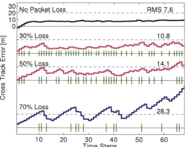
3-5 MIF-LQG control tests with acoustic communications on a day with light wind, 27 November 2012 . . . 49 3-6 MIF-LQG control tests with varying packet loss on a day with nearly no
wind, 24 October 2012 . . . 50 3-7 MIF-LQG control tests with varying packet loss on a day with strong wind,
16 October 2012. . . . 51 4-1 Block diagram for a MIMO feedback control system with an encoder,
bi-nary erasure channel, decoder, controller, and plant . . . 55 4-2 Block diagrams of SISO versions of the four codec algorithms . . . 63 4-3 Comparison of LZ (top left), LH (top right), LF (bottom left), and LM
(bottom right) blocks showing input and decoded signals. . . . 64 4-4 Block diagrams of SISO versions of the four codec algorithms with
4-5 Convergence of the LH describing function phase formula with g, for dif-ferent values of a, and or = 0.1. . . . 73 4-6 Convergence of the LM describing function phase formula with g, for
dif-ferent values of a, and (or = 0.1. . . . 74 4-7 Gain (top plot) and phase co of the LH model . . . . 75
4-8 Example 1-mass, 1-input 1-output system . . . 76
4-9 LF describing function gain (top plot) and phase (bottom plot) from analy-sis and Monte Carlo simulation, for the contact task example. . . . .. 77
4-10 Example 1-mass, 1-input 1-output inverted pendulum system . . . 78
4-11 LF describing function gain (top plot) and phase (bottom plot) from analy-sis and Monte Carlo simulation, for the inverted pendulum example. ... 79
4-12 Example 1-input, 1-output all-pass symmetric lattice circuit system. . . . . 80
4-13 LF describing function gain (top plot) and phase (bottom plot) from analy-sis and Monte Carlo simulation, for the nonminimum phase circuit example. 81
4-14 MIMO LF describing function gain (top plot) and phase (bottom plot) from analysis and Monte Carlo simulation, for the 2-sensor contact task example. 82
4-15 Example 2-mass, 1-input 2-output MIMO system . . . 83
4-16 MIMO LF describing function gain (top plot) and phase (bottom plot) from analysis and Monte Carlo simulation, for the 1-input 2-output double mass exam ple. . . . . ... . . . 84
4-17 Example 3-mass, 2-input 3-output, 6-state MIMO system . . . 85
4-18 MIMO LF describing function gain (top plot) and phase (bottom plot) from analysis and Monte Carlo simulation, for the 2-input 3-output three-mass example. Legend is same for both plots. . . . 86
4-19 LM gain (top plot) and phase co (bottom plot) from analysis and Monte Carlo simulation, for the contact task example. . . . 87
4-20 LM gain (top plot) and phase co (bottom plot) from analysis and Monte Carlo simulation, for the MIMO contact task example. . . . 88
4-21 LM gain (top plot) and phase a (bottom plot) from analysis and Monte Carlo simulation, for the 3-mass MIMO example. Legend is same for both plots . . . 89 4-22 Gain difference between coupled loss model and independent loss model
for two-channel LZ. . . . 90 4-23 Gain and phase differences between coupled loss model and independent
loss model for two-channel LH. . . . 91 4-24 Describing function gain N(a/h) for the uniform quantizer [32] with bin
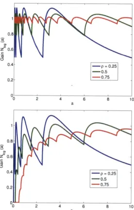
width h and input signal amplitude a . . . 92 4-25 Describing function gain for log quantizer as a function of input magnitude
a and quantizer parameter p for fine quantization (deadband p1000, top plot)
and coarse quantization (deadband p2, bottom plot). . . . 94 4-26 Block diagram for a MIMO feedback control system with a quantizer,
en-coder, binary erasure channel, deen-coder, controller, and plant . . . 95
5-1 Computation time for simulation and describing function for the SISO LZ decoder, for = -'r and a = 50% . . . 102
5-2 Computation time for simulation and describing function for the SISO LH
decoder, for r = -l and a = 50% . . . 103
5-3 Computation time for simulation and describing function for the SISO LF
decoder, for ar = -l and a = 50% . . . 103 5-4 Computation time for simulation and describing function for the SISO LM
decoder, for cor = -I and a = 50% . . . 104 5-5 Computation time for simulation and describing function for the SISO LM
decoder computing normalized bode plot gains, for 100 frequencies and a = 50% . . . 104
5-6 Gain (top) and phase (bottom) of the QLF for the contact task model; a =
10% , h = 46, T= 0.1. . . . 106
5-7 Gain (top) and phase (bottom) of the QLF for the contact task model; a =
5-8 Gain (top) and phase (bottom) of QLH; as with LH, these properties are
independent of the plant or controller. a = 10%, h = 46, r = 0.1. . . . 108
5-9 Gain (top) and phase (bottom) of QLH. a = 60%, h = 10, -r = 0.1. . . . 108
5-10 Block diagram of feedback control loop with additive disturbance on plant output. . . . 109
5-11 Gain of the sensitivity function for the contact task model with the QLF codec . . . 110
5-12 Closed-loop step response of double-integrator example system, with LQG design and a one-step delay. . . . 111
5-13 Input amplitudes a and quantization levels h that result in a limit cycle for the double-integrator example system . . . 112
5-14 Time series for the QLZ system with quantization level h = 70. . . . 113
5-15 Time series for the QLH system with quantization level h = 35 . . . 114
5-16 Frequency o of limit cycles from the analysis and from simulation . . . 114
6-1 Block diagram of SISO control system with binary erasure channel in sen-sor feedback, and describing function for the quantizer-encoder-channel-decoder. . . . 118
6-2 Example 1-mass, 1-input 1-output system . . . 132
6-3 Step responses of original system (top plot) and system with 1.1-second de-lay in sensor feedback (bottom plot). Nondimensional time is used, defined as gO. T*tim e. . . . 135
6-4 Nyquist plots for original system (top plot) and system with 1.1-second delay in sensor feedback channel (bottom plot). Nondimensional time is used, defined as gO r* time. . . . 136
6-5 Time series plots for QLZ (top) and QLH (bottom). Nondimensional time is used, defined as gor* time. . . . 137
6-6 Plot of limit cycle amplitudes for QLZ, QLH, and designed codecs. Blue dots represent design points. . . . ... . . . 138 6-7 Nyquist plots for system with decoder and delay but no loss or quantization 139
6-8 Limit cycle magnitudes as a function of M and N . . . 141 6-9 Sensitivity magnitude plots for original system and designed systems DI,
D2, and D3, with and without delay . . . 144
6-10 Describing-function-derived gain and phase loci of system with delay, loss, quantization, and designed codec . . . 146 6-11 Time series of system with designed decoder. Nondimensional time is
used, defined as gOw * time. . . . 147
6-12 Step responses of original system (top plot) and system with 1.1-second delay in sensor feedback (bottom plot) . . . 148 6-13 Example system with two inputs and four outputs . . . 152 6-14 Time response of original system to initial position displacements of 1 for
each mass, and initial velocities zero. Nondimensional time is used, defined 2
as gcO T*tim e. . . . 156 6-15 Loop transfer functions magnitudes for MIMO example, at low
frequen-cies. . . . 157 6-16 MIMO Nyquist plots for original system (top plot) and system with
1.5-second delay in sensor feedback channels (bottom plot) . . . 158 6-17 Time series responses of original system with 1.5-second time delay in
sensor feedback of all channels, for initial displacements of one for each mass and zero initial velocities. Nondimensional time is used, defined as
2
g T *tim e. . . . .159
6-18 MIMO design time series plots using QLZ codec . . . 160 6-19 MIMO design time series plots using QLH codec . . . 161 6-20 Plot of limit cycle amplitudes for states X1 and X2 for QLZ, QLH, and
designed codecs . . . 163 6-21 Nyquist plots of designs DI (top), D2 (middle) and D3 (bottom) for systems
with no nonlinearities (i.e.systems with delay and decoder but no loss or quantization) . . . 164 6-22 Nyquist plots of designs D4 (top) and DFinal (bottom) for systems with no
6-23 Describing-function-derived gain-phase loci of designed system with de-lay, quantization, and packet loss . . . 167 6-24 MIMO design time series plots using designed codec . . . 169
6-25 Time series responses of original system with no delay, loss, or
quantiza-tion with decoder . . . 170 6-26 Time series responses of original system with delay but no loss or
quanti-zation with decoder . . . 171 6-27 Transfer functions magnitudes for MIMO example with designed decoder,
at low frequencies. . . . 172
6-28 Quantizer gain plots. Top plot shows gain at a/h=0.6 corresponds to gain at larger value of a/h=0.9 . . . 173 6-29 Plot of limit cycle amplitudes for states Xi and X2 for QLZ, QLH, and
designed codecs . . . . . 174
6-30 Sensitivity plots of mean square limit cycle amplitude for small changes in
M decoder parameters. Red dot marks design point. . . . 175
6-31 Sensitivity plot of X1 and X2 limit cycle amplitudes for changes in M4
de-coder parameter. Red dots mark design point. . . . 176 6-32 Sensitivity plots of mean square limit cycle amplitude for small changes in
N decoder parameters. Red dot marks design point. . . . 177
6-33 Sensitivity plot of mean square limit cycle amplitude for large changes in N4 decoder parameter. Red dot marks design point. . . . 178
7-1 Experimental test setup . . . 180 7-2 Experimental test platform side view . . . 181 7-3 Experimental test platform top view, as seen from overhead camera. . . . . 181 7-4 Block diagram of experimental system. . . . 182 7-5 Actuator describing function capturing deadband (u <0.1), unity gain(0. 1 <
u < 1), and saturation (u > 1) regimes. . . . 183
7-6 Top view of autonomous raft used in experiments, showing thrusters and coordinate frame. . . . 184
7-7 Raft model vs data for thruster propeller speed step inputs of 30, 50, 70 and 90 percent . . . 185 7-8 Nyquist plot of loop transfer function with one time step delay. Crossover
is at -0.59. . . . 187 7-9 Example time series response of system to initial error of approximately-35
degrees, for one time step delay in sensor measurement. . . . 187 7-10 Nyquist plot of loop transfer function with three time step delay. . . . 188 7-11 Example time series response of system to initial error of -35 degrees, for
three time step delay in sensor measurement. . . . 189 7-12 Analytically predicted and experimentally observed limit cycle amplitudes. 191 7-13 Regions of different dominating factors influencing limit cycles. . . . 191 7-14 Experimentally observed limit cycle of magnitude approximately 1.9 for
pure quantizer, no packet loss. . . . 192 7-15 Experimentally observed limit cycle of magnitude approximately 1 for pure
quantizer, no packet loss. . . . 193 7-16 Experimentally observed limit cycle of magnitude approximately 0.8 for
QLZ with 15% packet loss. . . . 193 7-17 Experimentally observed limit cycles of magnitude approximately 1.8 for
QLH with 55% packet loss. . . . 194 7-18 Bode-like plots for the describing function of the designed codec. . . . 196 7-19 Describing-function-derived gain-phase loci for system with designed
con-troller with 25% packet loss and quantization ratio a/h = 0.9 . . . 197 7-20 Nyquist plot for system with designed controller with no packet loss or
quantization. . . . 198 7-21 Experimental time response for system with designed controller and delay,
with no quantization or packet loss. . . . 199 7-22 Limit cycle in experiment with designed controller/codec for 25% packet
List of Tables
3.1 Comparison of RMS errors from experiments with light wind and with strong w ind. . . . 51 4.1 Summary of mathematical symbols used in this chapter. . . . 54 6.1 Summary of mathematical symbols used in this chapter. . . . 118 6.2 Time series responses for system with no delay, delay, and delay+loss+quantization,
for LZ, LH, and designed decoders . . . 133 6.3 Nyquist plot for system with and without delay, for LZ, LH, and designed
decoders . . . 134 6.4 Codec coefficients and limit cycle amplitudes . . . 138
6.5 Gain and phase margins of system with delay and different decoders, with no loss or quantization. . . . 142 6.6 Time series responses for system with no delay, delay, and delay+loss+quantization,
for LZ, LH, and designed decoders. Nondimensional time is used, defined 2
as gO J T*time. . . . 154 6.7 Nyquist plot for system with and without delay, for LZ, LH, and designed
Chapter 1
Introduction
In this chapter we introduce the real-world problem that has motivated this thesis: con-trolling robotic systems where sensor signals are subject to packet loss and quantization errors. A statement of the problem is given in Section 1.1 with several applications, and a statement of the contributions of this thesis given in Section 1.2. A review of relevant prior work is given in Chapter 2.
1.1
Motivation and Problem Statement
Wirelessly connected robotic systems have become widespread in the terrestrial, aerial and underwater environments. Examples include autonomous underwater vehicle (AUV) coor-dination and navigation([1 1], [3], [33]), network-based process control engineering ([117])
, automobile networked subsystems control ([50], [21]), and power grid control ([106],[7 1],
[105]). As one would expect, demand on throughput grows to fill the available channel
ca-pacity; in a clean short-range RF setting, entire images may be transferred in each cycle, as part of a vision-based control system, whereas in the ocean, acoustic channels with per-haps twenty bits per second allow only the most basic sensor and command information to be shared regularly. Packet-based wireless communication systems like these that op-erate near their limits are necessarily quantized, and often prone to loss. These properties directly impact the overall system performance, and thus methodologies for understanding and designing feedback systems with quantization and packet loss are valuable.
1.1.1 Underwater Applications
Many example applications exist in underwater environments, where autonomous under-water vehicles (AUVs) are beginning to perform tasks previously done by human divers or remotely operated vehicles. AUVs have the advantage of requiring no tether, and not en-dangering the lives of divers, but communication underwater between the AUV and remote sensors or other AUVs may be subject to packet loss and quantization.
One application is AUV navigation through challenging environments using remote-sensor positioning measurements. Some of the most commonly-used remote-remote-sensor sys-tems for this application are Long Baseline (LBL) and Ultra-Short Baseline (USBL)[68].
Figure 1-1: Schematic of Long baseline system with AUV. Image credit: itime, http://www.km.kongsberg.com/ks/web/nokbg0240
Kongsberg
Mar-In the LBL setup, shown schematically in Figure 1-1, fixed nodes on the sea floor take acoustic range measurements to the AUV, triangulate the position, and acoustically transmit the position back to the AUV. LBL systems are currently used in AUV positioning for survey and inspection of deep water oil and gas facilities [102]. They have also been used to precisely position nuclear submarines navigating through underwater canyons or
preparing to launch missiles [34].
Figure 1-2: Schematic of ultra short baseline system with ROV and AUV. Image
credit: Teledyne Benthos, http: //www. benthos . com/index. php /product/
positioning-systems/benthos-dat
In the USBL setup, shown schematically in Figure 1-2, a surface vessel uses a hull-mounted underwater transceiver with multiple acoustic transducers to detect the range and angle to an underwater vehicle. The underwater vehicle emits a time-stamped acoustic signal, and the transceiver on the ship calculates range from the signal travel time. The multiple transducers receive different phase shifts of the same signal, and these phase dif-ferences are used to calculate the angle to the target. The ship can calculate the position from the range and angle measurements, and transmit this measurement acoustically back to the underwater vehicle. USBL positioning is currently used for AUV surveying and in-spection of underwater oil and gas facilities [102], and has the advantage that no additional underwater nodes need to be installed prior to operations.
Another underwater application is AUV collaborative positioning, where multiple AUVs must communicate with each other acoustically to perform a task. One example task could be teams of AUVs decommissioning offshore oil rigs. Offshore oil rigs are generally aban-doned at the end of their operational life, and in the United States oil companies are required to remove the rig within a year of abandonment. Current practice is to use a combination of human divers and Remotely Operated Vehicles (ROVs) to decommission and remove an old rig, but this is very dangerous for the divers, and ROV tether management can be problematic. An alternative method under research is to replace the divers and ROVs with AUVs, thus removing the danger to humans and the problems associated with tethers. This
may require AUVs to communicate acoustically to coordinate cutting and lifting tasks, and the communications could thus be subject to packet loss and quantization errors.
In these underwater applications both packet loss and quantization could be significant at the same time. For instance, if an acoustic modem used for communication has only a few different transmission modes (as is realistic), then the operation is limited to one of those modes and it may not be possible to configure the system such that only packet loss is significant or only quantization is significant. Thus the case of both significant quantization and packet loss is realistic for these applications.
1.1.2
Terrestrial Applications
Many terrestrial applications exist where networks of sensors are wirelessly connected and subject to packet loss [104]. Such a system can be advantageous if sensors are located far away from the plant, or if space is limited such that extensive wiring is undesirable. However, the network introduces the possibility of packet loss and quantization errors in signals.
These systems are used, for example, in some modem automobiles using using Control-Area-Network (CAN)-based data communication [117]. In this case space is very limited, and sensors for anti-lock braking systems, acceleration slip regulation, etc. are connected wirelessly to controllers over a network.
Satellite
Controller
Power Grid
Figure 1-3: Schematic of Wide Area Measurement System (WAMS).
These systems have also been used in power systems applications ([106],[71]) to main-tain power grid stability and prevent blackouts. In these cases, phasor measurement units (PMUs) are installed strategically in power grids to measure AC phases and waveforms,
and measurements are transmitted over a network using satellites to a controller, as shown in Figure 1-3. This is referred to as a Wide Area Measurement System (WAMS). As pointed out in [105], power systems are often operated close to their limits of stability due to eco-nomic and environmental pressures and deregulation, thus the effect of packet loss and quantization from WAMS could be significant if it pushed the system into a limit cycle or to instability.
In process control, such as in wastewater treatment plants, senors measuring water lev-els, pH factors, temperature, and chemical oxygen demand transmit signals through a net-work to a system controller [117]. In all of these applications, signals in the feedback control loop are subject to packet loss and quantization induced by the network.
Loss of a sensor measurement can also be caused at the sensor itself, and have the same effect as if it were lost in the feedback channel. For instance, automated welding for manufacturing is often controlled via visual servoing, though this is subject to sensor error from optical disturbances [119]. Arc glares, welding spatters, and smoke can all cause the sensor measurement to be effectively lost, even though it is not sent through a lossy communication channel.
1.2 Overview and Contributions of the Thesis
The goal of this thesis is to study the performance of feedback control systems limited by significant finite static quantization and stochastic packet loss. Unlike previous studies, the performance metric of this work is limit cycles - i.e., self-induced oscillations in nonlinear systems. Limit cycles are central in the performance of robotic and other systems because they dictate the precision which can be achieved. As will be shown, systems that are close to instability can be pushed into undesirable limit cycling by the combination of packet loss and significant finite quantization.
In Chapter 2 we review existing methods from the literature for designing and analyzing feedback control systems subject to quantization and packet loss. We also review describ-ing functions - quasi-linear approximations to non-linear system components - and some relevant applications in recent research. We then outline how describing functions can be
used to approximate the non-linear effects of quantization and packet loss, and in turn be used to analyze limit cycles.
In Chapter 3 we show experimental results from tests of a packet-loss robust algorithm
- the modified information filter - from the literature. Heading control tests are conducted on a robotic kayak in open water, with the sensor measurements transmitted to the kayak using a shore-based acoustic modem and subject to realistic packet loss. These tests are similar to true USBL-based control of an AUV, and serve as motivation for more detailed experiments in a controlled lab setting. These experimental results are also documented in [33].
In Chapter 4 we derive describing functions for information channels subject to packet loss and quantization. These are each given as closed-form mathematical expressions of the provably-optimal gains and phases for each case, with each decoder a specific case of the general codec algorithm. First, a DF is derived for a general codec of a channel subject to just packet loss. The general DF is then applied to four commonly-used codecs from the literature: Zero-Output, Hold-Output, Linear Filter, and Modified Information Filter. These DFs are verified by simulation for open-loop stable, open-loop unstable, minimum phase, and nonminimum phase SISO system examples, as well as for multi-sensor channels of several different MIMO system examples. The DFs are then combined with a standard quantizer DF to give DFs for channels subject to both quantization and packet loss.
These DFs build on the DF methods of the literature for studying nonlinear physical elements in control loops, and the new DFs are unique because they describe information sent through channels, and the information itself is stochastic. These two properties of the DF - describing non-physical and stochastic elements - distinguish the analysis from previous work and open the possibility for DF analysis to be applied to a much broader range of systems than has been standard practice in the past.
In Chapter 5 we show how the DFs require orders of magnitude less computation time than do simulations for computing gains and phases for quantized and lossy information channels. The DFs are shown to be useful analysis tools to create loop sensitivity-like functions to study the effect of disturbances, and to create channel Bode-like gain and phase plots. The.Bode-like plots can in turn be used to predict limit cycles of the system,
and a numerical example is given outlining this procedure. The example shows a case where the new DFs predict limit cycles in a quantized lossy system that are not predicted by a quantizer DF alone. The limit cycles are then shown by simulation to indeed exist.
In Chapter 6 we show how the DFs can be used as synthesis tools to design a channel codec. In this design procedure we assume two operating conditions for the system: a nom-inal operating case and a second operating case that is close to instability. This could apply, for instance, to an underwater vehicle navigating via LBL where a nominal operating case is in open water, while a second case is operating in a cluttered environment where acoustic signal performance is negatively affected, and quantization and packet loss push the sys-tem to limit cycle. For this synthesis tool, a controller is first designed for the nominal operating case, and an acceptable limit cycle amplitude specified for the second operating case. The design method gives a decoder that meets the limit cycle requirement with small effect to the nominal operating performance. The design method can be iteratively applied for smaller limit cycle amplitude specifications, until a balance is met that achieves small enough limit cycle amplitudes with acceptable effect on nominal operating performance.
The designed codec is of the special and simple form of a constant times the sent signal if the signal is received and a different constant times the previous decoded signal if the sent signal is lost. This form has the equivalent structure and computational complexity as the Zero-Output and Hold-Output decoders. A DF for this codec allows the constants to be solved for as functions of target limit cycle amplitudes. The constants reduce to solutions of cubic equations, which are guaranteed to have a real root, and thus the codec is physically realizable. The codec allows for multiple limit cycle frequency solutions for the same amplitude solution. SISO and MIMO numerical examples are given illustrating the design procedure.
In Chapter 7 we show experimental results on a small robotic raft. We control raft heading in an indoor pool environment and artificially add packet loss and quantization to the heading sensor measurements. The example codecs are implemented on the raft, and limit cycles predicted by the DFs are verified for a range of packet loss scenarios. A new design point is then selected where the system limit cycles at a smaller amplitude than any of the example codecs for a given packet loss probability. The design method is used to
achieve this design point, and verified experimentally. The results demonstrate how the designed decoder can be used to decrease limit cycle amplitudes even when compared to a linear-filter-based decoder.
We conclude in Chapter 8 by reviewing the contributions of the thesis and discussing areas of potential future work.
1.3 Assumptions
For clarity, we summarize the major assumptions used in the analysis and examples of the thesis:
* Discrete time control.
" Loss and quantization in sensor feedback channel.
" Uniform quantizer used.
" Bernoulli packet loss.
" No acknowledgments.
1.4 Example Systems Studied
In order to verify and illustrate the describing functions, we study an example set of linear open-loop stable, open-loop unstable, minimum phase, and nonminimum phase SISO sys-tems, and linear, minimum-phase, mass-spring-damper MIMO syssys-tems, and we list these example systems here for clarity:
" 1-mass with one force input (Section 5.5).
" 1-mass with spring and damper, with one force input (Section 4.4.3, 4.4.4).
" Open-loop unstable inverted pendulum (Section 4.4.3).
* 2 masses connected with springs and dampers, with one force input 4.4.4).
* 2 masses connected with springs and dampers, 4.4.4).
* 3 masses connected with springs and dampers, 4.4.4).
1.5 Summary
(Section 4.4.3,
with two force inputs (Section 4.4.3,
with two force inputs (Section 4.4.3,
This chapter described the importance of feedback control systems that are subject to packet loss and quantization. Example systems described include underwater vehicle navigation and coordination using acoustic communication, and power grid control. The contributions of this thesis to the control of these types of systems were then given, and the chapters of the thesis outlined.
Chapter 2
Background
2.1 Introduction
This chapter gives a survey of prior work in control systems subject to quantization and packet loss, as well as work related to describing functions. We begin with an overview of work related to control with quantization, followed by work related to control with packet loss and then work on a combination of the two. We then review recent applications of describing functions, and give background on control of underwater vehicle thrusters. We close with a synopsis of the background work and explain how describing function analysis fits into the existing research on packet loss and quantization.
2.2 Control with Quantization
The use of quantization in control systems has been studied at least since the 1950s, when Kalman [51] observed that quantized signals cause a stabilizing controller to exhibit limit cycles and chaotic behavior. Since then, work on quantizers has fallen into two basic categories: work studying static (also called memoryless) quantizers, and work studying dynamic quantizers (also called quantizers with memory). A static quantizer maintains the same parameters (such as bin sizes and location) over time, while for a dynamic quantizer these properties are allowed to vary over time. Curry [17], Miller [67], and Delchamps [19] gave early results on the effect of static uniform quantizers on control systems, and
Wong [112] determined bounds on the number on uniform quantization intervals needed to practically stabilize a linear system. However, a finite uniform quantizer can do no better than practical stability. To achieve quadratic stability with a static quantizer Elia [23] proved that, at least in the case of a SISO system, the quantizer must be logarithmic with infinite precision. This type of quantizer is, of course, not practically realizable. Fagnani [24] looked at methods to reach practical stability for SISO systems with more practical static finite logarithmic quantizers.
Brockett [12] developed one of the first results using dynamic quantizers, showing that dynamic finite quantizers can in fact achieve asymptotic stability, unlike static finite quan-tizers. Several works later studied bounds on the number of dynamic quantization levels needed for closed loop quadratic (Ling [60] and Nair [74]) and exponential ([75]) stability. Fu ([29] and [30]) developed a unique dynamic logarithmic quantizer that scales a gain on
the quantizer parameters.
Currently one of the most common means of dealing with quantization in feedback control is to use the sector bound method developed by Fu ([28], [27]). In this method, quantization error is treated as uncertainty and bounded using a sector bound. By doing this, the quantization error can be considered to be additive noise, and standard control analysis tools can be applied to study and minimize the quantization effect. Fu used the sector bound method to determine stabilizability and H. performance criteria for SISO and MIMO systems. Coutinho [16] used the sector bound approach to quadratically stabilize a system using infinite logarithmic quantizers in sensor and controller channels. Bai [4] developed a set of bilinear matrix equations for system stability, for MIMO systems with different quantization in different channels, and Rasool [85] extended these results to in-clude H. performance criteria. Wei [109] modified the sector bound method to account for multiplicative noise instead of additive.
The sector bound method developed by Fu is, however, conservative in stability con-ditions. Less conservative approaches using quantization-dependent Lyapunov functions (Gao [31]) have also been developed.
A final method to deal with quantization is to look at it from an information theoretic view. Tatikonda [100] used this method, and determined the minimum bit rate required to
achieve stability and control objectives.
2.3 Control with Packet Loss
Much work has been done in the past 50 years studying the important problem of control systems subject to packet loss. Most work focuses on how to design the encoder, decoder, and/or controller to attain some stability or performance result. Some of the first work, by Nahi [73] and Hadidi [41] studied SISO systems with packet loss in the sensor feedback channel and acknowledgments. They derived an optimal codec scheme where a linear com-bination of current and past measurements are sent if a measurement is lost, with Bernoulli or Markov loss probability. Robinson [87] extended these results to include system perfor-mance criteria. Other methods of dealing with packet loss include treating lost packets as long delays (Zhang [118]), and looking at the system's output power spectral density as a function of packet loss (Ling [59]).
One of the most common ways to deal with packet loss in the sensor channel is to use a Kalman Filter decoder, where a state estimate is propagated through a system model if the measurement is lost, and a Kalman gain is multiplied by the difference between measure-ment and propagated model if the measuremeasure-ment is received. Sinopoli [92] and Fortmann
[25] found critical packet loss probabilities for error covariance matrix convergence in this
case.
Many variations exist on the standard Kalman-Filter setup. Several authors (Smith [97], Nilsson [77], [76], and Costa [15]) extended the Kalman Filter results to look at jump lin-ear estimator decoders [65] that select a gain from a fixed set depending on whether the measurement packet was received. This type of decoder was shown to be less computa-tionally expensive than the standard Kalman filter. Wang [108] and Schenato [89] designed general constant-gain linear filter decoders that bound the estimation error covariance by a prescribed amount.
Another useful variant of the Kalman Filter that has been studied for these problems is the information filter. Gupta [40],[39] developed a modified information filter codec for sensor channel loss that involves sending a specialized information vector, which depends
on current and past measurements and state estimates. This was shown to be the optimal LQG-type control for losses in the sensor channel. Jin [49] and Jiang [48] considered the case where the sensor packet can be split up and sent through multiple independent channels, before being recombined and decoded with a Kalman Filter-type decoder, and Li
[58] studied the Unscented Kalman Filter under packet loss.
Fewer works have considered the scenario where only the controller-actuator channel is subject to packet loss. One of the simplest codec methods (Mahmoud [63]) is to send the single control command and decode with a zero-output or hold-output decoder. Quevedo [83] developed packetized predictive control (PPC), where a set of current and future con-trol commands is sent to the actuator at each step. If the signal is lost, the actuator uses the next control command stored in its buffer. Miklovicova [66] studied the specific PPC case where the controller is PID, and switches between gains based on whether the control command was successfully received (requiring acknowledgments). Song [98] and Yang [114] extended PPC to the MIMO case with mixed packet losses, called network predictive control.
Several works have considered the case where packet loss can occur in both the sensor-controller and sensor-controller-actuator channels. Most studies assume a Kalman Filter decoder for the sensor channel, and a zero-output decoder for the controller channel. Azimi-Sadjadi [1] developed one of the first results for this system, establishing LMI stability criteria, and Sinopoli [93] developed critical packet loss probability for convergence of the error covari-ance matrix. Schenato [90] showed that, if acknowledgments are used there is a critical packet loss probability for stability and that the separation principle holds, but the separa-tion principle does not hold in the case of no acknowledgments. Lu [62] and Yang [113] de-signed stable controllers that meet H. performance specifications for this system. Moayedi studied two variations on this control scheme, where control commands are encoded in a PPC manner [69], and when they are sent normally but with a hold-output decoder [70].
2.4 Control with Quantization and Packet Loss
Only in the past decade have studies considered the important real-world situation where quantization and packet loss exist simultaneously in a feedback control system. Branicky
et al. [10] was one of the earliest to include both quantization and packet loss in a
con-trol system analysis, developing a scheduling co-design method for Networked Concon-trol Systems (NCSs). Hadjicostis [42] treated quantization as additive noise on a signal and de-rived stability criteria for a simple SISO system with sensor channel packet loss. Tsumura
et al. [103] developed one of the first fundamental analyses for this problem, expressing
the minimum quantization level required for feedback stability for a given packet loss and open-loop unstable eigenvalues. The study assumed a log quantizer with a realistic dead-band at the origin, and required acknowledgments for the lossy sensor channel.
Niu et al. [78] later derived a set of linear matrix inequalities that guarantee feedback stability for packet loss and infinite-precision logarithmic quantization in the sensor chan-nel; this result was extended by Dai et al. [18] to include quantization and packet loss also in the controller channel. Liu [61] added random delays to the model, and Yang [115] considered different delays on different channels of a multi-channel system. In terms of closed-loop performance, Rasool and Nguang [84] recently introduced a variation where disturbance-to-penalty norm can be minimized, and Jiang [47] developed a set of LMI constraints that guarantee system stability and H. performance criteria. Guo [38] studied the case where the channel decoder is a general linear filter that propagates a model if the sensor measurement is lost.
Some studies assume quantization errors are small and treat them as sector-bounded additive noise. Huaicheng [45] used this treatment of quantization and developed LMI stability criteria for systems with mixed delays and mixed loss probabilities in the sensor feedback channel. Seiler [91] derived LMIs for synthesis of H. controllers for Markovian packet loss, and Chiuso [14] and Dey [20] designed LQR gain matrices. Mahmoud [63] developed stability conditions for the case of quantization and loss in both control and sensor channels, with non-stationary Bernoulli packet loss probabilities.
Na-gahara [72] extended the work of Quevedo [83] to send a sparse representation of the quantized signal, and Ishido [46] extended it to include a finite uniform quantization of the signal.
2.5
Limit Cycles
No previous works have looked at control systems subject to packet loss and quantization from the perspective of the effect on limit cycling. However, limit cycling is very important for many robotic systems because it is a measure of achievable precision. Limit cycles will not necessarily happen in all systems. For example, a system that is open-loop stable with a very mild controller may not exhibit any limit cycles. Systems that are operated closer to instability, though, may be prone to limit cycling in the presence of packet loss and quantization, as will be described later in more detail.
There are three main methods from the literature used to find limit cycles: Bendixson's Theorem, contraction theory, and describing functions. Bendixson's Theorem states that if a region of state space has no trajectories leaving it, then trajectories must go to limit-ing sets, which are either equilibrium points or limit cycles [36]. The theorem has been used to prove stability of some systems such as biological cellular concentrations [64] and formation-keeping for mobile agents [5]. However, it does not give insights into the limit cycle characteristics. Contraction theory is similar to Bendixson's Theorem in many ways, and states that a system moves to a unique trajectory when initial conditions or distur-bances are forgotten exponentially fast. Contraction has been used to study limit-cycling of coupled nonlinear oscillators, e.g., [107].
A describing function (DF) is a quasi-linear approximation to a nonlinear element, and depends explicitly on the form of its input; for sinusoidal signals in a limit cycle, the DF depends on the input frequency or amplitude, or both [32]. DFs are very practical tools for real-world control applications, and have been described as "an indispensable component in the bag of tools of practicing control engineers" [95]. It is for this practical reason that we choose to use DFs for limit cycle analysis of systems subject to packet loss and quantization.
DFs have been used successfully in many applications. To name a few, in electrical en-gineering Sanders [88] studied limit cycles in periodically-switched circuits, and Peterchev
et al. [81] found quantization conditions that eliminate limit cycles in digitally-controlled
PWM converters. In medicine, Kinnane [56] used DFs to predict blood pressure oscilla-tions in human patients for diagnosing cardiovascular health. In control, E. Kim et a]. [52] developed a DF for a fuzzy logic controller, and Kim et al. [54] used DFs for identifying frictional elements in support of feedforward control action. In ocean engineering, Yoerger
et al. [116] used DFs to explain and reduce limit cycles in underwater robots caused by
nonlinear thruster dynamics. More details about control of underwater thrusters is given in Section 2.6.
More recently, DFs have been widely applied to stability analysis of airfoils (e.g., Tang
et al. [99]) and flame formation in combustion, e.g., Noiray et al.[79]. Gelb and Vander
Velde [32] provide a good resource, with many other DFs for a wide range of applications, and Taylor [101] gives examples of calculating DFs for multiple-input-multiple-output sys-tems. It is noteworthy that these prior works all address DFs for hardware and physical elements, but not for information sent across channels, our current focus. Our work is also unique in that the dynamic element whose describing function is to be developed is itself
stochastic.
2.6 Control of Underwater Thrusters
Because the contributions of this thesis have many applications in the control of underwater vehicles, it is important to review previous work on ROV and AUV control. As pointed out in Section 2.5, a key difficulty in controlling underwater vehicles is compensating for nonlinear thruster behavior, which affects vehicle positioning. A variety of methods exist in the literature to model and control underwater thrusters.
2.6.1
Thruster Modeling
In general in steady state the thrust from the thruster is proportional to the square of the propeller rotational velocity. However, in the transient state this simplified model does not
hold as well. One approach to model the transient state thrust is to derive an equation of motion by using an energy balance to equate axial power at the propeller disk to power expended at the propeller shaft [116]. This leads to a nonlinear differential equation relating propeller velocity to thrust. Another modeling method is to include the motor in the model, with a voltage or current input [43]. A momentum balance can then be used to relate thrust to propeller velocity. The input command can also be assumed to be propeller velocity [110], which avoids taking into account motor voltages and currents. A more detailed modeling approach is also possible, which takes into account variables such as propeller blade angles, blade lift and drag forces, and fluid dynamics [43].
These modeling methods assume a model is derived in advance, but other methods allow for the possibility of model parameters changing over time. Several studies ([2], [26]) developed techniques for adaptively identifying model parameter values in real time. These methods, however, generally require measuring axial fluid velocity, which is difficult to do in practice. One method approximates axial flow by a function of ambient flow velocity and propeller shaft velocity, which are easily measurable, thus allowing parameters to be identified in real time [53].
2.6.2 Thruster Control
The simplest, and a very common, framework to control underwater thrusters is open-loop control with no feedback. This understandably may not meet performance requirements, for instance in the case of strong disturbances, and perhaps the next step up in complexity is feedback velocity control [111]. In this method the thrust is approximated to be linearly proportional to the propeller velocity, which can be measured. Another approach is model-based velocity control, where one of the many nonlinear relationships between thrust and propeller velocity is assumed, and a measurement of axial flow velocity is also used. One more approach is to use an extended Kalman filter to estimate motor torque, then estimate thrust from this torque estimate and a hydrodynamic model [37].
Many different types of controllers can be applied to these general control frameworks. For instance LQR [35], neural-network [55], integral [44], and
proportional-derivative [96] controllers have all been tested either in simulation or experiment on ROVs or AUVs. More recently, fuzzy sliding mode controllers have been studied for underwa-ter thrusunderwa-ter control ([8],[9],[7]). In these controllers the compensator gain is variable and determined by a fuzzy inference system. Such a design can be more robust to parametric uncertainties and can deal with realistic motor deadband, but is prone to chatter and may reduce system precision.
2.7 Synopsis of Literature Review
Most of the previous studies that consider both packet loss and quantization rely on infinite-length logarithmic quantizers with no lower bound on precision, and this makes their ap-plication to severely limited channels tenuous. Also, in these works all signals in a channel are assumed lost or passed together, with no consideration of a mixed-loss scenario. The channel decoders are generally assumed to be one of three specific algorithms: zero-output, hold-output, or linear filter. It is unclear if stability or performance results hold if a different decoder is used than the specific one assumed in each study.
Works that assume finite quantization levels generally assume quantization error is small enough to be treated as additive noise. However, if quantization error is large, it is not clear that the treatment as additive noise holds. Additive noise will not effect the Nyquist plot of a system, but, as will be shown later, coarse quantization does effect the Nyquist plot of a system, and thus is not well-approximated by the additive noise assumption.
Studies that assume coarse finite quantization generally use dynamic quantizers, but dy-namic quantizers don't necessarily work with packet loss. A dydy-namic quantizer inherently relies on information being exchanged between the quantizer and receiver any time the quantizer changes. If the channel being used is subject to random packet loss, implement-ing a dynamic quantizer becomes more difficult. If the sendimplement-ing side changes the quantizer parameters, but the message specifying the new parameters gets dropped en route to the receiving side, the receiving side will not correctly decode future messages.
One way to ensure the message successfully reaches the receiving side is to use ac-knowledgments, i.e. to send a signal from the receiving side confirming that it has received
the new quantizer parameters. This strategy relies on the acknowledgment signal not being dropped in the channel. Acknowledgments are commonly used in transmissions over the internet using Transmission Control Protocol (TCP) [82]. This strategy works in transmis-sions over the internet because, in general, the acknowledgment message is much smaller than a standard message and much less likely to be dropped by the channel. However, in underwater acoustic communication this assumption that the acknowledgment will not be dropped does not always hold. In general, smaller packets have a smaller probability of being dropped, but in the underwater environment the possibility of an acknowledgment signal being dropped cannot be ignored. Thus dynamic quantization is not always possible in channels subject to packet loss.
With respect to underwater systems, many studies have focused on controlling under-water vehicles in the face of nonlinear thruster dynamics, and somehave looked at the effect of limit cycles induced by these thruster nonlinearities. However, no works have considered the effect of packet loss and quantization on limit cycling of underwater vehicles, though these nonlinearities are potentially significant in many underwater feedback control appli-cations such as those pointed out in Section 1.1.1. While thruster dynamics, packet loss, and quantization could all potentially contribute to limit cycling at the same time, this the-sis is concerned with the case where packet loss is high enough and/or quantization coarse enough that the packet loss and quantization effects dominate the limit cycling.
This thesis thus advances previous work by considering systems with both significant finite quantization and packet loss from the perspective of limit cycling, with applications to underwater vehicle control.
2.8 Summary
In this section we reviewed prior work on control systems subject to quantization and packet loss, as well as work related to limit cycles and underwater vehicle control. Most previous works treat quantization errors as small, or assume infinite-precision logarithmic quantizers. Work that considers both packet loss and quantization often assumes acknowl-edgments can be used. All of these assumptions may not hold in the case of severely
limited channels. Also, no previous work has studied control systems subject to packet loss and quantization from the perspective of limit cycling. This review motivates the work of this thesis, which considers feedback control subject to significant finite quantization and packet loss from the perspective of limit cycling, with applications to underwater vehicle control.