The dynamics of invariant object and action
recognition in the human visual system
by
Leyla Isik
B.S., Johns Hopkins University, 2010
Submitted to the Program of Computational and Systems Biology in partial fulfillment of the requirements for the degree of Doctor of Philosophy in Computational and Systems Biology
at the
MASSACHUSETTS INSTITUTE OF TECHNOLOGY June 2015
Massachusetts Institute of Technology 2015. All rights reserved.
A uthor ...
Certified by..
Signature redacted
v IProgram of Conputational and Systems Biology May 22, 2015
Signature redacted
...
Tomaso Poggio Professor of Brain and Cognitive Sciences Thesis SupervisorAccepted by...
Signature redacted
Chris Burge
Professor of Biology and Biological Engineering
Director, Computational and Systems Biology Graduate Program
MASSACHUSETTS INSTITUTE OF TECHNOLOLGY
JUN 11 2015
The dynamics of invariant object and action recognition in
the human visual system
by
Leyla Isik
Submitted to the Program of Computational and Systems Biology on May 22, 2015, in partial fulfillment of the
requirements for the degree of
Doctor of Philosophy in Computational and Systems Biology
Abstract
Humans can quickly and effortlessly recognize objects, and people and their actions from complex visual inputs. Despite the ease with which the human brain solves this problem, the underlying computational steps have remained enigmatic. What makes object and action recognition challenging are identity-preserving transformations that alter the visual appearance of objects and actions, such as changes in scale, position, and viewpoint. The majority of visual neuroscience studies examining visual recog-nition either use physiology recordings, which provide high spatiotemporal resolution data with limited brain coverage, or functional MRI, which provides high spatial res-olution data from across the brain with limited temporal resres-olution. High temporal resolution data from across the brain is needed to break down and understand the computational steps underlying invariant visual recognition.
In this thesis I use magenetoencephalography, machine learning, and computa-tional modeling to study invariant visual recognition. I show that a temporal associa-tion learning rule for learning invariance in hierarchical visual systems is very robust to manipulations and visual disputations that happen during development (Chap-ter 2). I next show that object recognition occurs very quickly, with invariance to size and position developing in stages beginning around 100ms after stimulus onset (Chapter 3), and that action recognition occurs on a similarly fast time scale, 200 ms after video onset, with this early representation being invariant to changes in actor and viewpoint (Chapter 4). Finally, I show that the same hierarchical feedforward model can explain both the object and action recognition timing results, putting this timing data in the broader context of computer vision systems and models of the brain. This work sheds light on the computational mechanisms underlying invariant object and action recognition in the brain and demonstrates the importance of using high temporal resolution data to understand neural computations.
Thesis Supervisor: Tomaso Poggio
Acknowledgments
First I would like to thank my advisor Tomaso Poggio. Tommy, before I even came to MIT your work inspired my interest in artificial intelligence and neuroscience. It has been amazing to work with you. Your encouragement gave me the confidence to first try MEG experiments, and take advantage of many other new and exciting opportunities I would not have otherwise. Thank you for everything.
Next I would like to thank my thesis committee: Robert Desimone, Nancy Kan-wisher, and Gabriel Kreiman. Your insightful feedback, as well as the excitement and energy you brought to our discussions has had a tremendous impact on me and my work.
I would like to thank all my friends in the Poggio lab for fruitful collaborations
and many fun times. Particularly to my wonderful collaborators - Andrea Tacchetti,
Ethan Meyers, Joel Z. Leibo, Danny Harari and Yena Han - you are all amazing and
I have learned so much from working with each of you. Steve Voinea, Owen Lewis and Youssef Mroueh, thank you for your friendship over the years (and awesome feedback on this thesis). Kathleen Sullivan, Felicia Bishop, Elisa Pompeo, thank you for all of your help and support. Gadi Geiger, thank you for great coffee and many welcome distractions.
I would also like to thank Chris Burge and Jacquie Carota, as well as all of my
friends in the CSB program. Thanks to the wonderful GWAMIT community - you
all have made my MIT experience so much better. And to my awesome living groups: the Warehouse and Baker House.
I would like to thank the rest of my friends and my family. Dan Saragnese, thank
you for encouraging me in all of my endeavors, both large and small. I don't know what I would do without your support. Finally, I would like to thank my parents, Salwa Ammar and Can Isik, for instilling the importance of knowledge and learning in me, as well as my brother Sinan. All of your love and encouragement helps me in everything I do. I could not have done this without you.
Contents
1 Introduction 15
1.1 State of the field . . . . 16
1.1.1 Visual recognition in the brain . . . . 16
1.1.2 Timing in the brain . . . . 19
1.1.3 Visual recognition with convolutional neural network models . 21 1.2 Background methods . . . . 24
1.2.1 M E G . . . . 24
1.2.2 Neural decoding analysis . . . . 26
1.2.3 H M AX . . . . 27
1.3 Contributions . . . . 27
1.3.1 Main contributions . . . . 27
1.3.2 Organization of this thesis . . . . 28
2 Robustness of invariance learning in the ventral stream 31 2.1 Introduction . . . . 32
2.2 Temporal association learning with the cortical model . . . . 33
2.2.1 Learning rule . . . . 35
2.3 Robustness . . . . 36
2.3.1 Training for translation invariance . . . . 36
2.3.2 Accuracy of temporal association learning . . . . 36
2.3.3 Manipulating the translation invariance of a single cell . . . . 37
2.3.5 Robustness of temporal association learning with a population
of cells . . . . 2.4 Discussion . . . .
3 The dynamics of size- and position-invariant the human visual system
3.1 Introduction . . . . 3.2 Materials and Methods . . . . 3.2.1 Subjects . . . .
3.2.2 Experimental Procedure . . . .
3.2.3 Eyetracking . . . .
3.2.4 MEG recordings and data processing .
3.2.5 Decoding analysis methods . . . .
3.2.6 Significance criteria . . . . . . . . 39 . . . . 41 object recognition in 45 . . . . 46 . . . . 47 . . . . 47 . . . . 47 . . . . 49 . . . . 49 . . . . 49 . . . . 52 3.2.7 Significance testing with normalized decoding magnitudes.
3.2.8 Source localization . . . .
3.2.9 Cortical modeling (HMAX) . . . .
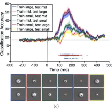
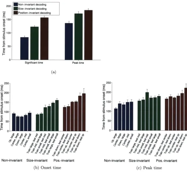
3.3 R esults . . . . 3.3.1 Fast and robust readout for different types of stimuli . . . 3.3.2 Timing of size and position invariant visual representations
3.3.3 Varying extent of size and position invariance . . . .
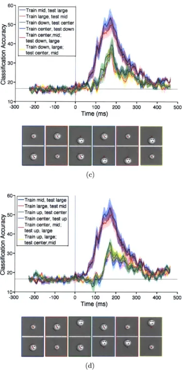
3.3.4 Combined size- and position-invariance . . . .
3.3.5 Dynamics of decoded signals . . . .
3.3.6 Neural sources underlying sensor activity and classification
3.3.7 Invariant recognition with a cortical model . . . .
3.4 D iscussion . . . .
3.5 Appendix - Decoding in source space . . . .
3.5.1 M ethods . . . .
3.5.2 R esults . . . .
3.5.3 Source estimates at key decoding times . . . .
52 53 53 54 54 57 58 61 64 68 68 70 74 75 76 76
3.5.4 D iscussion . . . . 78
4 Invariant representations for action in the human brain 83 4.1 Introduction . . . . 84
4.2 R esults . . . . 85
4.2.1 Novel invariant action recognition dataset . . . . 85
4.2.2 Readout of actions from MEG data is early and invariant . . . 86
4.2.3 Extreme view invariance . . . . 89
4.2.4 Recognizing actions with a biologically-inspired hierarchical model 89 4.2.5 Recognizing actor invariant to action . . . . 95
4.2.6 The roles of form and motion in invariant action recognition . 96 4.2.7 Neural sources of action recognition . . . . 97
4.2.8 Generalization to novel actions with a fixed model . . . . 101
4.3 D iscussion . . . . 102
4.3.1 Fast, invariant action recognition and implications for model architecture . . . . 102
4.3.2 Actor invariance and recognition . . . . 103
4.3.3 Neural sources underlying invariant action recognition . . . . . 103
4.3.4 Form and motion in invariant action recognition . . . . 104
4.3.5 Conclusion . . . . 105
4.4 M ethods . . . . 105
4.4.1 Action recognition dataset . . . . 105
4.4.2 Subjects . . . . 106
4.4.3 MEG experimental procedure . . . . 106
4.4.4 MEG data acquisition and preprocessing . . . . 106
4.4.5 Eyetracking . . . . 107
4.4.6 MEG decoding analysis methods . . . . 107
4.4.7 Source localization . . . . 108
4.4.8 Model .... ... .. .. ... ... ... .. .... .109
4.4.10 Model experiments . . . 110
4.5 Supplemental figures . . . . 112
4.5.1 CI model performance on action recognition dataset . . . . . 112
4.5.2 Effect of eye movement on action decoding . . . . 113
5 Conclusions 115 5.1 Summary of findings . . . . 115
5.1.1 Temporal association training is a robust method for learning invariance in development . . . . 115
5.1.2 Size- and position-invariant object recognition have fast dynam-ics that match feedforward models of visual cortex . . . . 116
5.1.3 Actor- and viewpoint-invariant action representations arise quickly and match a feedforward model of visual cortex . . . . 117
5.1.4 Common themes . . . . 117
5.2 Future directions . . . . 118
5.2.1 Moving towards more naturalistic vision experiments . . . . . 118
5.2.2 Combining temporal and spatial information in the human brainl19 5.3 Conclusion . . . . 120
List of Figures
Timing in the macaque ventral stream . . . .
The HMAX model . . . . 2-1 An illustration of the HMAX model with normal and altered temporal association training . . . . 2-2 Image recognition with hard-wired model and temporal associate learn-ing m odel . . . .
2-3 Manipulating single cell translation invariance through altered visual
experience .. . . . . 2-4 Translation invariance for different model population cell sizes . . . .
Experimental Task . . . . Decoding accuracy versus time for three different image sets Decoding parameter optimization . . . . Assessing position and size invariant information . . . . Significant and peak invariant decoding times . . . . Assessing combined size and position invariant information . Dynamics of object decoding . . . . Source localization at key decoding times . . . . Invariant image classification with a cortical model . . . . .
20 22 34 37 38 40 1-1 1-2 3-1 3-2 3-3 3-4 3-5 3-6 3-7 3-8 3-9 . . . . . 48 . . . . . 55 . . . . . 57 . . . . . 60 . . . . . 62 . . . . . 66 . . . . . 67 69 . . . . . 71
3-10 A left view of source estimates on cortex of subject 1 at 70ms after
stimulus onset, the time when image identity can first be decoded, and
150 ms after stimulus onset, the time when size- and position-invariant
information can be decoded. Color bar right indicates absolute source
magnitude in picoAmpere-meters. . . . . 77
3-11 Comparison of decoding in sensor and source space . . . . 80
3-12 Decoding within visual ROIs . . . . 81
4-1 Novel action recognition dataset . . . . 86
4-2 Decoding action . . . . 87
4-3 Decoding action invariant to actor and viewpoint . . . . 88
4-4 "Extreme" view-invariant decoding . . . . 90
4-5 Biologically inspired computational model for action recognition . . . 92
4-6 Model pooling across viewpoints . . . . 93
4-7 Model performance on view-invariant action recognition . . . . 94
4-8 Decoding actor from MEG data . . . . 95
4-9 Model performance on action-invariant actor recognition . . . . 96
4-10 The roles of form and motion in MEG action decoding . . . . 98
4-11 Model performance on static frames . . . . 99
4-12 Neural sources of action recognition . . . . 100
4-13 Generalizing to recognize new actions . . . . 101
4-14 C1 model performance on action recognition dataset . . . 112
List of Tables
3.1 Decoding accuracy magnitude, significant time, and peak times with varying amounts of data . . . . 63
Chapter 1
Introduction
Humans can process complex visual scenes within a fraction of a second [138, 171, 42, 139, 140]. The main computational difficulty in visual recognition is believed to be transformations that change the low-level representation of objects and actions, such as changes to size, viewpoint, and position in the visual field [32, 5]. The ability to effortlessly discount these transformations and learn from few examples make the human visual system superior to even state of the art computer vision algorithms. Better understanding the neural mechanisms underlying visual recognition in humans will greatly improve artificial intelligence (AI) systems and provide insight into how the brain solves one of the most complex sensory problems.
Studies using single neuron and neural population recordings have provided high spatiotemporal resolution data about object and action recognition, but their coverage is limited to recording from one or two brain regions at a time. fMRI studies have improved our understanding of the spatial organization of the brain and functional regions of interest; however, fMRI its still limited in its temporal resolution.
Understanding when different invariant representations are computed across the brain is a crucial component missing from many neuroscience efforts, and will help further our understanding of the algorithms underlying visual recognition. In order to break down the computational steps required to solve the complex problem of visual recognition, it is important to know what the intermediate steps are (to go from pixels/retinal response to invariant representations of objects and actions) and
when and in what order they are computed. This thesis focuses on when and how different properties of invariant recognition are computed in the brain, using mag-netoencephalography (MEG), machine learning, and computational models of the human visual system.
The remainder of this chapter describes the state of the field for object and action processing in the brain, as well as an overview of state of the art computer vision systems and biologically plausible models of the human visual cortex. Finally, it provides some details on the methods used in this thesis.
1.1
State of the field
1.1.1
Visual recognition in the brain
Visual signals enter the brain via the retina and lateral geniculate nucleus (LGN) and first enter the cortex in the primary visual cortex (V1). The visual cortex has been
roughly divided into two pathways -the ventral (or "what") pathway, which processes
objects, and the dorsal (or "where") pathway, which processes actions and spatial location [121, 57]. This distinction is somewhat of an oversimplification as there are many interconnections and feedback between areas in both pathways [44, 116]. Despite these complexities, the visual cortex is still considered to be hierarchically organized with the responses of one visual layer, serving as input to the subsequent layer.
Object recognition occurs along the ventral stream. We consider the initial visual response to be occurring in a primarily feedforward manner with connections proceed-ing from visual area V1 to V2 to V4 to inferior temporal cortex (IT), see Figure 1-1. Invariance and selectivity increase at each layer of the ventral stream [10, 147, 152]. In the dorsal stream, visual signals also originate in V1, where cells are selective for local, directed motion. These motion signals then enter area MT, where cells are selective for motion direction invariant to pattern [122], and neural responses have been closely linked with motion perception [36, 3]. MT then projects to areas MST
and FST in the superior temporal sulcus (STS) [175, 31, 791.
Object processing along the ventral stream
Beginning with Hubel and Wiesel's seminal studies in V1 [761, single-cell physiology studies have helped explain many properties of the ventral stream. Hubel and Wiesel showed in the cat and the macaque that cells in VI fire in response to oriented lines or edges, and are selective for a given orientation [77, 781. They also discovered two different cell types within V1: simple and complex cells. V1 simple cells are selective (or "tuned") for a given feature (i.e. a line or edge of a given orientation) within a small receptive field. Complex cells receive input from these simple cells and compute an aggregate measure (or "ipool") over these features to provide invariance over the union of the simple cells' receptive fields. Due to the retinotopic organization of
Vi, by pooling over neighboring simple cells, complex cells achieve selectivity to a
given feature within a particular spatial region, providing local position invariance (see Figure 1-2 for a model diagram of this process).
Mid-level object and shape representations have been harder to explain than those in V1. Cells in V2 share many properties of shape response with V1 cells and they are also selective to orientation and spatial frequency [73, 74, 8, 38]. It has also been shown that V2 cells are sensitive to higher order statistical dependencies than V1, which may play a role in recognizing image structure [50]. Cells in V4 appear to have more complex shape representations including polar, hyperbolic and Cartesian gratings [54, 551, contours and curvature [129], and complex shape and color [154, 96, 145]. The final layer of the primate ventral stream, IT, is generally divided into a posterior portion and an anterior portion. The posterior portion is selective to object parts and partially invariant, and cells in the anterior portion are selective to complex objects, including faces, and invariant to a wide range of scale and position changes
[61, 29, 28, 168, 132, 167].
fMRI studies over the last two decades have revealed similar organization for the human ventral stream [39, 186, 72, 9], and that the transition from low-level statistics to object-level information increases gradually along the ventral stream [581.
In addition, there exist several object-specific regions in visual cortex, which respond preferentially to certain ecologically relevant categories, including faces, places, and bodies [90, 41, 35, 130, 60]. Recent studies have shown that these object-selective regions exist in the macaque, and fMRI-guided physiology has been used to show correspondence with object-selective single cells [173, 84].
Recordings from IT neurons and voxels in object-selective cortex reveal these areas are remarkably invariant to a range of transformations, including not only affine transformations such as changes in size and position [85, 80, 21], but also non-affine transformations such as changes in illumination and viewpoint [113, 59, 111, 51, 16].
All objects undergo affine transformations in the same manner (e.g. they scale and
translate in the same manner), so a neural mechanism used to deal with these types of invariance can, in principle, be used for all objects. This is not true of non-affine transformations, such as rotation in depth, which depend on the 3-D structure of an individual object or class of objects, and thus must be learned for each class of objects
[180, 13, 105].
Action recognition in the brain
As they do with objects, humans can also recognize actions very quickly, even from very impoverished stimuli. Action recognition, however, has been much less studied than object recognition, and the majority of action recognition studies are focused on experiments with simple, controlled stimuli. These stimuli are mostly static images, which contain only form information, or point light displays (created by placing dots on the joints of a moving human), which contain biological motion information with little to no form information [88].
Previous experiments using such stimuli revealed that neural representations for biological motion exist in the macaque STS [141, 133, 127, 179], and in a posterior region of the STS in humans (pSTS) [62, 63, 177, 14, 130]. The STS is a long sulcus that spans the temporal lobe, and receives input from both the ventral and dorsal streams. The STS has also been implicated in general motion processing, face recognition, and social perception [31, 19, 4, 69, 153, 53].
Actions can also be recognized from static images, and in general this elicits similar activity in motion-selective areas, including MT/MST [97] and STS, as well in the extra striate body area (EBA), a region traditionally considered to be more involved in form processing [120, 110].
In addition to distinguishing biological motion types of motion, fMRI studies have also shown that pSTS can distinguish between different types of actions [178], and can do so in a mirror symmetric manner [64]. Physiology studies have found that neurons in the macaque STS can identify both action invariant to actor and actor invariant to action, showing that the same neural population can be both selective and invariant to each of these features [159].
The computational steps required to go from oriented lines and edges to invariant representations of whole objects, or from directed motions to actions (particularly from natural video stimuli), are still largely unknown. The timing of different stages of visual processing can help explain these underlying neural computations.
1.1.2
Timing in the brain
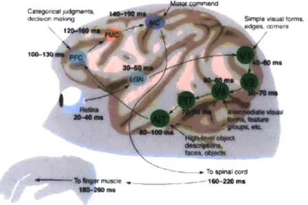
Most timing information known about the primate ventral stream comes from electro-physiological studies of macaques. Latencies of visual areas along the ventral pathway are known in the macaque, ranging from 40-60ms in V1 to 80-100ms in IT, and timing between each area is approximately 20 ms [126, 155, 172, 801 (see Figure 1-1). These latencies, however, are still largely unknown in humans.
Some recent work using electrocorticography (ECoG) in human patients with pharmacologically intractable epilepsy has provided the rare opportunity to record from the surface of the human brain. These studies have shown that, as in the macaque, human visual signals that are invariant to size and position exist after 100 ms [111]. ECoG methods are limited by the lack of spatial coverage, and the scarcity of eligible subjects.
The majority of human timing results have come from noninvasive studies ex-amining evoked responses in electroencephalography (EEG), and to a lesser extent,
SImrpl v*iuai forms,
edges, comers
- - To spinal cord
'muscie .-- 1_2____
EU m.
Figure 1-1: A diagram outlining the timing of different steps in the macaque brain to during a rapid object categorization task. Visual areas along the ventral stream are highlighted in green. The latencies of the visual areas along the ventral stream have been measured in the macaque. Figure modified from [172].
(distinguishing between scenes with or without animals) very quickly, with reaction times as fast as 250 ms, and divergence in EEG responses evoked by the two cate-gories occurring at 150ms [171]. In addition, object-specific signals, such as the N170 response to faces, a strong negative potentiation in certain EEG channels 170 ms after image onset in response to faces versus non-faces [15], have a similar latency. It has been shown that the N170 response is also elicited by facial and body movements
[187].
Using MEG decoding, others have shown that high-level categorization can be performed, such as distinguishing between two categories of objects (faces vs. cars) [21] or higher-level questions of animacy vs. inanimacy [22, 24], around 150ms. These signals occur late relative to those in the macaque summarized above [126, 155, 172,
80] (Figure 1-1). These results raise the question: what are computational stages in
1.1.3
Visual recognition with convolutional neural network
models
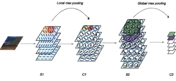
Hubel and Wiesel's findings in visual cortex, namely that there are simple cells that are feature selective and complex cells that pool over simple cells to build invariance, have inspired a class of computer vision models. These models consist of a hierar-chical organization of alternating convolutional or "tuning" layers and subsampling or "pooling" layers. The convolutional layers perform template matching between a given feature (e.g. an oriented Gabor filter, as found in V1 simple cells) and over-lapping regions of an input image (analogous to cells' receptive fields in the visual field). The pooling layers perform a max (or other pooling operation) to build in-variance over that pooling range (e.g. if a complex cell pools over several simple cells that are selective for the same orientation, that complex cell will be selective for that orientation feature anywhere in its pooling range, invariant to position) and reduce sample complexity (the number of training examples needed to learn a new category) [5, 191] (see Figure 1-2). These models can be broken into two categories, biologically-inspired models and performance-optimizing deep neural networks, based on their architecture and training procedure. (It is important to note that the term "deep neural network" refers to any algorithm that uses many layers of feature extrac-tors and uses the outputs of one layer as input to the next, and not necessarily deep convolutional neural networks, which are one specific type of deep neural network. In this chapter, we will use "deep neural networks" to refer to the specific type of deep convolutional neural networks.)
Biologically-inspired computer vision models
The first type of model, biologically-inspired, was introduced by Fukushima
[52].
The models' architecture and parameters are set to closely model properties of cells in the visual cortex, and they are usually trained in an unsupervised manner to mimic natural visual experience [184, 144, 157, 174, 1881. These models have been expanded to recognize actions from videos, by including a temporal component to the templates
Local max poong GlotAm max pooflng
S1 Ci S2 C2
Figure 1-2: An outline of the HMAX model, one type of biologically-inspired convo-lutional neural network, adapted from [1561. The model consists of alternating layers of simple 'S' cells, which are tuned for a particular feature (oriented lines in the case of SI and more complex shapes sampled from natural images in S2), and complex 'C' cells which pool over the responses of 'S' cells to build invariance. (The pooling range for a given C1 or C2 cell are highlighted for illustration.) The final C2 feature vector for each image can be compared to the response of a population of IT cells and used to classify images into different categories.
and pooling [56, 87], and to recognize faces invariantly to non-affine transformations (e.g. rotation in depth, changes in background) 1105, 109]. A particular instantiation of these Hubel and Wiesel-inspired (HW) models used in this research, known as the HMAX model, is described in section 1.2.3 and Figure 1-2.
In these models, the pooling regions are hard-wired, which raises the question of how these arise in the brain? People have proposed theories for how these invariant representations may be learned in development by taking advantage of the fact that objects typically move in and out of the visual field much slower they transform, and linking temporally adjacent views of the same object [49, 146, 189, 37, 162]. A recent computational theory has suggested that learning how a few objects transform in development and storing "templates" for their transformed views can lead to trans-formation invariance for novel objects [5]. This theory further explains why these
hierarchical networks have achieved such success at object recognition, and states that the main goal of cortical hierarchies is to encode invariant representations of objects. Further, these invariant representations decrease the sample complexity for recognition - i.e. allow the brain to learn from few labeled examples [6, 7].
Deep convolutional neural networks
In recent years the second type of neural network models, deep neural networks, have achieved unprecedented human-level performance on a series of vision challenges, in particular, on the object recognition challenge ImageNet, a 1000 category categoriza-tion problem which includes thousands of training images per category and over 14 million total images [160, 43, 151]. In 2012, the winner of the ImageNet challenge em-ployed a deep neural network, which outperformed other systems by a unprecedented extent
[99].
Today, most high-performing computer vision systems employ these deep neural networks. These convolutional neural networks were pioneered almost 30 years ago [150, 137, 103, 104], and again were inspired loosely by the architecture of brain and the model of Fukushima [52]. While the recent success of these algorithms is undeniable, it seems to be in large part due to the availability of better comput-ing power and the prevalence of large traincomput-ing sets of example images, rather than any changes to the networks architecture[991.
One key distinction with the above biolgically-inspired models is that these networks' architecture and parameters are set for performance rather than biological fidelity. In particular, the weights in the network are learned through "back-propagation" the process of using gradient descent to propagate error signals on training data to update the weights.As with object recognition, deep convolutional networks are also the top perform-ing computer vision systems on action recognition tasks [101, 93]. In the case of action recognition though, these systems do not achieve the same high, human-like performance as they do with objects (they achieve 40-80% accuracy instead of over
90% achieved on the ImageNet Challenge). It is still unclear if the performance of
deep neural networks on action recognition tasks will improve as more large datasets of labeled videos are created.
In addition to their high performance on computer vision tasks, deep neural networks have shown a remarkably high correspondence with primate neural data
[192, 18]. The top stages of these networks are able to explain most of the variance in
IT recordings, and middle network layers show similarly high correspondence with V4 neurons, both of which have been notably challenging to model. This work suggests that the performance optimizing aspects of these deep neural networks are solving the same optimization as the brain. Surprisingly, this work has even shown that these models predict neural responses even better than models fit with neural data. This is likely due to the fact that there is not enough neural data to constrain such large and complex models.
Despite the recent success of deep neural networks, their basis on the architecture of the brain, and correspondence with neural data, there are several ways in which these algorithms are distinctly different from, and arguably inferior to, human vision. Primarily, these models require thousands of labeled examples to learn a new class of objects, while children and adults can learn a new category of object from only a few labeled examples [20, 114, 190]. Second, while some work has been done to address higher-level tasks (such as image captioning and narration) it is unclear how many tasks beyond visual categorizations can be explained by these models. The goal of many recent neuroscience and AI research efforts is to find new discoveries that will, just as previous neuroscience insights have inspired the above algorithms, further propel progress towards more intelligent and human-like computer vision systems.
1.2
Background methods
1.2.1
MEG
With the complexity of the visual system, one would ideally record simultaneously with high spatiotemporal resolution from across the visual cortex. Unfortunately, this is infeasible with today's recording technologies. Here we focus on measuring high temporal resolution data with broad brain coverage using MEG. As mentioned
above, these two aspects in concert have been understudied and can provide great insight into the brain's computations. Specifically, timing data can help explain how (in what order) invariant representations are computed, which can constrain existing and inspire new algorithms for object and action recognition.
MEG is a direct, non-invasive measure of whole-head neural firing with millisecond
temporal resolution. EEG and MEG detect the electrical and magnetic fields, respec-tively, that are produced by synchronous neural firing. MEG requires on the order of 50 million neurons oriented in the same direction to fire synchronously, and thus detects signals primarily from pyramidal neurons aligned perpendicular to the sur-face of the cortex. Due to the geometry of the cortical sursur-face and resulting magnetic fields, MEG is primarily sensitive to neural sources in the sulci and EEG primarily detects activity primarily from the gyri. Unlike electric fields detected with EEG, magnetic fields are not impeded by the skull and scalp 1102], and thus MEG is a less noisy measure of neural activity.
Typical MEG methods involve analyzing event-related fields evoked by a cer-tain stimulus. This is done by presenting a stimulus on the order of 100 times and averaging the value of the magnetic field measured in a given channel over the multi-ple stimulus repetitions to improve the signal-to-noise ratio. This has led to several discoveries of visual timing hallmarks, described in section 1.1.2 [171, 151. This proce-dure, however, has several notable drawbacks, mainly that it requires several stimulus repetitions, is not a direct measure of and is limited by the univariate nature of the analysis.
Source localization methods are often used in conjunction with this event-related field analysis to estimate where the neural sources driving MEG or EEG measure-ments are located. Source localization, however, is an ill-posed problem. Even when taking into account geometric constraints of cortical shape and orientation of mag-netic fields, there are still orders of magnitude more sources one tries to estimate than sensor measurements that are made with MEG. This limits the spatial resolution of
MEG. The most widespread way to overcome the ill-posed nature of the problem is
estimate [67, 11]. This minimum norm estimate minimizes the total power of the
sources, which has little physiological basis. Other methods that impose sparsity of the sources by regularizing with Li or L1-L2 norm combinations have also been used
[66]. Recent results have shown that incorporating fMRI data into source
estima-tion methods can greatly improve the spatial resoluestima-tion of MEG/EEG measurements
[1281. Other new methods have also taken advantage of the dynamic information in MEG to create better temporal models of the inverse problem [100].
Neural decoding analysis is a tool that can be applied to source- or sensor-level data and, unlike the above methods, provides a direct measure of stimulus information present in the data. Neural decoding has been largely unexplored for analyzing MEG visual data.
1.2.2
Neural decoding analysis
Neural decoding analysis uses a machine learning classifier to assess what information about the input stimulus is present in the recorded neural data (for example, what image the subject was looking at). Decoding analysis has the advantage of being able to extract information from the pattern of neural activity across multiple sensors or voxels, and as a result has increased sensitivity over univariate analyses [80, 68, 94,
131].
Decoding analysis, or multi-voxel pattern analysis (MVPA), has been widely used in fMRI visual research and led to great progress in predicting visual cortical response to a range of visual stimuli [68, 89, 70, 94, 185], and even reconstructing visual stimuli purely based on fMRI data [125]. Decoding analysis has also been applied to electro-physiology visual data [80, 119, 193], and to a lesser extent to EEG and MEG visual data. MEG decoding has been used recently to show category-selective signals with some position invariance present at 150 ms [21], and other properties about objects, such as animacy/inanimacy, between 150-200 ms [22, 24].
One main advantage of neural decoding is that it makes it possible to test for the presence of invariant information in the visual signals. By training the classifier on stimuli presented at one condition (a given, position or scale, for example), and
testing on a second condition (a different position or scale), it is possible see if the neural information can generalize across that transformation. This technique has been applied to fMRI data [701, electrophysiology data [80, 193], and MEG data [211.
1.2.3 HMAX
HMAX falls in the class of Hubel and Wiesel-inspired models described above in section 1.1.3. One particular instantiation consists of two layers of alternating simple and complex cells. The first simple cell layer, S1, contains features or templates that are Gabor filters of varying scales and orientations. A dot product is computed between each of the Gabor filters at each location in the image (a convolution). In the first complex cell layer, C1, a local maximum is computed across position and scales to provide invariance in these local regions. In the second simple cell layer, S2, the templates are drawn from random natural image patches that are fed through the S1 and C1 layers of the HMAX model, which serve as an intermediate layer feature. In the final C2 layer, pooling is performed for each feature across all sizes and positions to provide global size and position invariance (Figure 1-2). The final C2 vector can then be used as input to a machine learning classifier trained on various tasks, such as object recognition. This model has been shown to match human performance on a feedforward object categorization task where images are masked to prevent feedback
processing
11571.
Some key questions about this model remain: how biologically faithful is it, namely is there evidence that the brain employs this alternating tuning and pooling beyond V1? And to what extent and on what subset of tasks do these feedforward models explain human visual performance?
1.3
Contributions
1.3.1 Main contributions
" Visual signals containing information sufficient for object recognition exist as
early as 60 ms after stimulus onset in the human visual system.
* Size and position invariance begin at 100 ms after stimulus onset, with invari-ance to smaller transformations occurring before invariinvari-ance to larger transfor-mations.
" Action selective visual signals occur as early as 200ms after video onset.
* These early representations for action are also invariant to changes in actor and viewpoint.
" The same feedforward, hierarchical models for visual recognition can explain
both these object and action recognition timing results.
1.3.2
Organization of this thesis
Chapter two implements a temporal association learning rule, a popular computa-tional mechanism for learning invariance in development, in the HMAX model. Sim-ulations with this model demonstrate the robustness of this learning mechanism. We find that, as in recent behavioral and physiology studies, we can learn and subse-quently disrupt position invariance in single model units through temporal associa-tion learning. Despite this single cell disrupassocia-tion, a populaassocia-tion of cells remains robust to these manipulations, demonstrating the fidelity of this learning rule across many neurons.
Chapter three describes the dynamics of size- and position-invariant object recog-nition in the human brain. Using MEG decoding, we show that object identity can be read out in 60ms, with invariance to size and position invariance increasing in stages between 100-150 ms. These results uncover previously unknown latencies for human object recognition, and compelling evidence for a feedforward, hierarchical model of the visual system.
Chapter four describes the dynamics of viewpoint invariant action recognition in the brain and an accompanying computational model. Here we use video stimuli to
better examine realistic visual input and understand how the brain uses spatiotem-poral information to recognize actions. We show that, like object recognition, action recognition is also fast and invariant, with a representation for action that is invariant to actor and view arising in the brain in around 200 ms. We extend the same class of hierarchical feedforward computational model to account for these MEG results. Finally we show that, like the MEG signals, the model can recognize action invariant to actor and view.
Chapter five concludes the thesis by examining common themes in this work and future directions for using temporal dynamics to understand visual computations in the brain.
Chapter 2
Robustness of invariance learning in
the ventral stream
This material in this chapter was published in Frontiers in Computational Neuro-science in 2012 [82]. Joel Z. Leibo and I contributed equally to this work.
Learning by temporal association rules, such as Foldiak's trace rule [49], is an at-tractive hypothesis that explains the development of invariance in visual recognition.
Consistent with these rules, several recent experiments have shown that invariance can be broken by appropriately altering the visual environment. These experiments raise puzzling differences in the effect size and altered training time at the
psychophys-ical [26, 1831 versus single cell [107, 108] level. We show a) that associative learning provides appropriate invariance in models of object recognition inspired by Hubel and Wiesel [76], b) that we can replicate the "invariance disruption" experiments using these models with a temporal association learning rule to develop and maintain invariance, and c) that we can thereby explain the apparent discrepancies between psychophysics and singe cells effects. We argue that this mechanism in hierarchical models of visual cortex provides stability of perceptual invariance despite the under-lying plasticity of the system, the variability of the visual world and expected noise in the biological mechanisms.
2.1
Introduction
Temporal association learning rules provide a plausible way to learn transformation invariance through natural visual experience [49, 115, 161, 184, 189]. Objects typically move in and out of our visual field much slower than they transform, and based on this difference in time scale the brain learns to group the same object under different transformations. These learning methods are attractive solutions to the problem of invariance development. However, these algorithms have mainly been examined in idealized situations that do not contain the complexities present in the task of learning to see from natural vision or, when they do, ignore the imperfections of a biological learning mechanism. Here we present a model of invariance learning that predicts the invariant object recognition performance of a neural population can be surprisingly robust, even in the face of frequent temporal association errors.
Experimental studies of temporal association and the acquisition of invariance involve putting observers in an altered visual environment where objects change their identity across saccades. Cox et al. showed that after a few days of exposure to this altered environment, the subjects mistook one object for another at a specific retinal position, while preserving their ability to discriminate the same objects at other positions [26]. A subsequent physiology experiment by Li and DiCarlo using a similar paradigm showed that individual neurons in primate anterior inferotemporal cortex (AIT) change their selectivity in a position-dependent manner after less than an hour of exposure to the altered visual environment [107]. It is important to note that the stimuli used in the Cox et al. experiment were difficult to discriminate "greeble" objects, while the stimuli used by Li and DiCarlo were easily discriminable,
e.g., a teacup versus a sailboat.
This presents a puzzle, if the cells in AIT are really underlying the discrimination task, and exposure to the altered visual environment causes strong neural effects so quickly, then why is it that behavioral effects do not arise until much later? The fact that the neural effects were observed with highly dissimilar objects (the equivalent of an easy discrimination task) while the behavioral effects in the human experiment
were only observed with a difficult discrimination task compounds this puzzle. The physiology experiment did not include a behavioral readout, so the effects of the manipulation on the monkey's perceptual performance is not currently known; however, the human evidence suggests it is highly unlikely that the monkey would really be perceptually confused between teacups and sailboats after such a short exposure to the altered visual environment.
We present a computational model of invariance learning that shows how strong effects at the single cell level do not necessarily cause confusion on the neural pop-ulation level, and hence do not imply perceptual effects. Our simpop-ulations show that a population of cells is surprisingly robust to large numbers of mis-wirings due to errors of temporal association. In accord with the psychophysics literature 126, 183], our model also predicts that the difficulty of the discrimination task is the primary determiner of the amount of exposure necessary to observe a behavioral effect, rather than the strength of the neural effect on individual cells.
2.2
Temporal association learning with the cortical
model
We examine temporal feature learning with the HMAX model [157, 144]. The results
presented should generalize to other models in the class of Hubel-Wiesel models
[52].
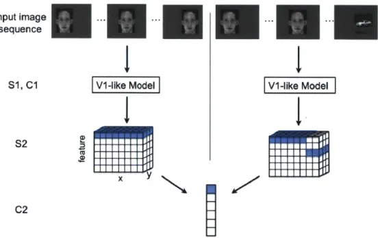
The model learns translation invariance, specifically in the S2 to C2 connections, from a continuously translating image sequence, as shown in Figure 2-1, left. During training, an image (face or car) is translated left to right over a time period, which we will call an "association period". During this association period, one C2 cell learns to pool over highly active S2 cells. Correct temporal association should group similar features across spatial locations, as illustrated in Figure 2-1, left. Potential "mis-wiring" effects of a temporally altered image sequence are illustrated in Figure 2-1, right.
Input image ...
sequence
S1, C1 V1-like Model VI-like Model
CC
C2
Figure 2-1: An illustration of the HMAX model with two different input image se-quences: a normal translating image sequence (left), and an altered temporal image sequence (right). The model consists of four layers of alternating simple and complex cells. S1 and C1 (Vi-like model): The first two model layers make up a Vi-like model that mimics simple and complex cells in the primary visual cortex. The first simple cell layer, S1, consists of simple orientation-tuned Gabor filters, and the fol-lowing complex cell layer, C1, performs max pooling over local regions of a given S1 feature. These are identical to the first two model layers in 1157]. S2: The next
sim-ple cell layer, S2, performs template matching between C1 responses from an input image and the C1 responses of stored prototypes (unless otherwise noted, we use pro-totypes that were tuned to natural image patches). Template matching is performed with a radial basis function, where the responses have a Gaussian-like dependence on the Euclidean distance between the (CI) neural representation of an input image patch and a stored prototype. The RBF response to each template is calculated at various spatial locations for the image (with half overlap). Thus the S2 response to one image (or image sequence) has three dimensions: x and y corresponding to the original image dimensions, and feature the response to each template. C2: The final complex cell layer, C2, performs global max pooling over all the S2 units to which it is connected. The S2 to C2 connections are highlighted for both the normal (left) and altered (right) image sequences. To achieve ideal transformation invariance, the
C2 cell can pool over all positions for a given feature as shown with the highlighted
2.2.1 Learning rule
In Foldiak's original trace rule, shown in Equation 2.1, the weight of a synapse between an input cell and output cell is strengthened proportionally to the input activity and the trace or average of recent output activity at time t. The dependence of the trace on previous activity decays over time with the 6 term [49].
Foldiak trace rule:
AW9 oC xiy
(2.1)
g(t = (1 - 6)y t1 + 6y?
In the HMAX model, connections between S and C cells are binary. Additionally, in our training case we want to learn connections based on image sequences of a known length, and thus for simplicity should include a hard time window rather than a decaying time dependence. Thus we employed a modified trace rule that is appropriate for learning S2 to C2 connections in the HMAX model.
Modified trace rule for the HMAX model: for t in T :
if xj > 6, wi = 1 (2.2) else, wij = 0
With this learning rule, one C2 cell is produced for each association period. The length of the association period is T.
2.3
Robustness
2.3.1 Training for translation invariance
We model natural invariance learning with a training phase where the model learns to group different representations of a given object based on the learning rule in Equation 2.2. Through the learning rule, the model groups continuously-translating
images that move across the field of view over each known association period T. An
example of a translating image sequence is shown at the top, left of Figure 2-1. During this training phase, the model learns the domain of pooling for each C2 cell.
2.3.2 Accuracy of temporal association learning
To test the performance of the HMAX model with the learning rule in Equation
2.2, we train the model with a sequence of training images. Next we compare the
learned model's performance to that of the hard-wired HMAX
[157]
on atranslation-invariance recognition task. In standard implementations of the HMAX model, each
C2 cell pools all the S2 responses for a given template globally over all spatial
loca-tions. This pooling gives the model translation invariance and mimics the outcome of an idealized temporal association process.
We test both models on a face vs. car identification task with 20 faces and 20 cars
that contain slight intraclass variation across different translated views1. We collect
hard-wired C2 units and C2 units learned from temporal sequences of the faces and cars. We then test each model's translation invariance by using a nearest neighbor classifier to compare the correlation of C2 responses for translated objects to those in a given reference position. The accuracy of the two methods (hard-wired and learned from test images) for different amounts of translation is shown in Figure 2-2. The two methods performed equally well, confirming that the temporal associations learned from training yield accurate invariance results.
'The training and testing datasets come from a concatenation of
two datasets from: http://www.d2.mpi-inf.mpg.de/Datasets/ETH80, and http://www.cl.cam.ac.uk/research/dtg/attarchive/facedatabase.html
1 0.95-0.9 0.85- 0.8-0.75 - 0.7- 0.65- 0.6-0.55 . -s-Hard-wired connections
I-*-Temporal
learning 0.5. 5 10 15 20 25 30 35 40 Translation (pixels)Figure 2-2: The classification accuracy (AUC for ROC curve) for both hard-wired and temporal association learning model plotted for different degrees of translation compared to a reference position with a nearest neighbor classifier. The model was trained and tested on separate training and testing sets, each with 20 car and 20 face images. For temporal association learning, one C2 unit is learned for each association period or training image, yielding 40 learned C2 units. One hard-wired C2 unit was learned from each natural image that cells were tuned to, yielding 10 hard wired C2 units. Increasing the number of hard-wired features has only a marginal effect on classification accuracy.
2.3.3
Manipulating the translation invariance of a single cell
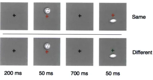
To model the Li and DiCarlo physiology experiments in [107] we perform normal temporal association learning described by Equation 2.2 with a translating image of one face and one car. The S2 units are tuned to (i.e. use templates from) the same face and car images as in the training set to mimic object-specific cells that are found in AIT. Next we select a "swap position" and perform altered training with the face and car images swapped only at that position (see Figure 2-1, top right). After the altered training, we observe the response of one C2 cell, which has a preference for one stimuli over the other (to model single cell recordings), to the preferred and non-preferred objects at the swap position and at a second, non-swap position that was unaltered during training.
Normal posibn tolerance Non- 0Swp swap posmon
P
-N -xpvP Fully altered po-ftn tolerance N es. Exposure -+(a) Figure from Li and DiCarlo 2008 1107] summarizing the ex-pected results of swap exposure on a single cell. P is response to preferred stimulus, and N is that td non-preferred stimulus.
0
-2 B
Before
- - preferred stim, swap position
-preferred stim, non-swap position
- - non-preferred stim, swap position
-non-preferred stim, non-swap position After Time point (before and after altered training)
(b) The response of a C2 cell tuned to a preferred object before (time point 1) and after (time point 2) altered visual training where the preferred and non-preferred objects were swapped at a given position. To model the experimental paradigm used in [107, 108, 26, 183], training and testing were performed on the same altered image sequence. The C2 cell's relative response (Z-score) to the preferred and non-preferred objects at both the swap and non-swap positions are plotted.
Figure 2-3: experience.
Manipulating single cell translation invariance through altered visual
As shown in Figure 2.3.3 the C2 preference has switched at the swap position: the response for the preferred object at the swap position (but not the non-swap position) is lower after training, and the C2 response to the non-preferred object is higher at
S
the swap position. As in the physiology experiments performed by Li and DiCarlo, these results are object and position specific.
2.3.4 Individual cell versus population response
In the previous section we modeled the single cell results of Li and DiCarlo, namely that translation invariant representations of objects can be disrupted by a relatively
small amount of exposure to altered temporal associations. However, single cell
changes do not necessarily reflect whole population or perceptual behavior and no behavioral tests were performed on the animals in this study.
A cortical model with a temporal association learning rule provides a way to model
population behavior with swap exposures similar to the ones used by Li and DiCarlo
[107, 108]. A C2 cell in the HMAX model can be treated as analogous to an AIT cell
(as tested by Li and DiCarlo), and a C2 vector as a population of these cells. We can thus apply a classifier to this cell population to obtain a model of behavior or perception.
2.3.5 Robustness of temporal association learning with a pop-ulation of cells
We next model the response of a population of cells to different amounts of swap exposure, as illustrated in Figure 2-1, right. The translating image sequence with which we train the model replicates visual experience, and thus jumbling varying amounts of these training images is analogous to presenting different amounts of altered exposure to a test subject as in 1107, 108]. These disruptions also model the mis-associations that may occur with temporal association learning due to sudden changes in the visual field (such as light, occlusions, etc), or other imperfections of the biological learning mechanism. During each training phase we randomly swap different face and car images in the image sequences with a certain probability, and observe the effect on the response of a classifier applied to a population of C2 cells. The performance, as measured by area under the ROC curve (AUC), versus different
neural population sizes (number of C2 cells) is shown in Figure 2-4 for several amounts of altered exposure. We measured altered exposure by the probability of flipping a face and car image in the training sequence.
1 0.9 - 0.8- 0.7-0.6 -prob switch = 0 -prob switch = 0.125 -prob switch = 0.25 -prob switch = 0.5 0.5 I I I I 20 30 40 50 60 70 80 90 100 Number of C2 units
Figure 2-4: Results of a translation invariance task (+/- 40 pixels) with varying amounts of altered visual experience. To model the experimental paradigm used in
[107, 108, 26, 1831, training and testing were performed on the same altered image
sequence. The accuracy (AUC for ROC curve) with a nearest neighbor classifier
compared to center face for a translation invariance task versus the number of C2 units. Different curves have a different amount of exposure to altered visual training as measured by the probability of swapping a car and face image in training. The error bars show +/- one standard deviation.
A small amount of exposure to altered temporal training (0.125 probability of
flipping face and car) has negligible effects, and the model under this altered training performs as well as with normal temporal training. A larger amount of exposure to
altered temporal training (0.25 image flip probability) is not significantly different than perfect temporal training, especially if the neural population is large enough. With enough C2 cells, each of which is learned from a temporal training sequence, the
effects of small amounts of jumbling in training images are insignificant. Even with half altered exposure (0.5 image flip probability), if there are enough C2 cells then