HAL Id: hal-02648825
https://hal.archives-ouvertes.fr/hal-02648825
Submitted on 29 May 2020HAL is a multi-disciplinary open access archive for the deposit and dissemination of sci-entific research documents, whether they are pub-lished or not. The documents may come from teaching and research institutions in France or abroad, or from public or private research centers.
L’archive ouverte pluridisciplinaire HAL, est destinée au dépôt et à la diffusion de documents scientifiques de niveau recherche, publiés ou non, émanant des établissements d’enseignement et de recherche français ou étrangers, des laboratoires publics ou privés.
A nonequilibrium thermodynamics perspective on
nature-inspired chemical engineering processes
Vincent Gerbaud, Nataliya Shcherbakova, Sergio da Cunha
To cite this version:
Vincent Gerbaud, Nataliya Shcherbakova, Sergio da Cunha. A nonequilibrium thermodynamics per-spective on nature-inspired chemical engineering processes. Chemical Engineering Research and De-sign, Elsevier, 2019, 154, pp.316-330. �10.1016/j.cherd.2019.10.037�. �hal-02648825�
OATAO is an open access repository that collects the work of Toulouse
researchers and makes it freely available over the web where possible
Any correspondence concerning this service should be sent
to the repository administrator:
[email protected]
This is an author’s version published in: http://oatao.univ-toulouse.fr/ 26045
To cite this version:
Gerbaud, Vincent and Da Cunha, Sergio and Shcherbakova, Nataliya A nonequilibrium
thermodynamics perspective on nature-inspired chemical engineering processes. (2019)
Chemical Engineering Research and Design, 154. 316-330. ISSN 0263-8762
Official URL :
https://doi.org/10.1016/j.cherd.2019.10.0371
A nonequilibrium thermodynamics perspective on
nature-inspired chemical engineering processes
Vincent Gerbaud
1*, Natalyia Shcherbakova
1, Sergio Da Cunha
11
Laboratoire de Génie Chimique, Université de Toulouse, CNRS, INP, UPS, Toulouse, France * corresponding author: [email protected]
Author accepted manuscript
Abstract
Nature-inspired chemical engineering (NICE) is promising many benefits in terms of energy consumption, resilience and efficiencyetc.but it struggles to emerge as a leading discipline, chiefly because of the misconception that mimicking Nature is sufficient. It is not, since goals and constrained context are different. Hence, revealing context and understanding the mechanisms of nature-inspiration should be encouraged. In this contribution we revisit the classification of three published mechanisms underlying nature-inspired engineering, namely hierarchical transport network, force balancing and dynamic self-organization, by setting them in a broader framework supported by nonequilibrium thermodynamics, the constructal law and nonlinear control concepts. While the three mechanisms mapping is not complete, the NET and CL joint framework opens also new perspectives. This novel perspective goes over classical chemical engineering where equilibrium based assumptions or linear transport phenomena and control are the ruling mechanisms in process unit design and operation. At small-scale level, NICE processes should sometimes consider advanced thermodynamic concepts to account for fluctuations and boundary effects on local properties. At the process unit level, one should exploit out-of-equilibrium situations with thermodynamic coupling under various dynamical states, be it a stationary state or a self-organized state. Then, nonlinear phenomena, possibly provoked by operating larger driving force to achieve greater dissipative flows, might occur, controllable by using nonlinear control theory. At the plant level, the virtual factory approach relying on servitization and modular equipment proposes a framework for knowledge and information management that could lead to resilient and agile chemical plants, especially biorefineries.
Keywords
Nature-inspired engineering; nonequilibrium thermodynamics; nonlinear control; self-organization; virtual modular factory
2
1 Introduction
Chemical engineering deals with the processing of matter and energy, which requires processing with information as well. It also puts an emphasis on the development of technologies used for the large-scale chemical production and on the manufacture of products with desired properties through chemical processes. Interactions within and between processes are important, as well as dynamics. But, like a cat, chemical engineering is purring over its assets. Most of models and knowledge in use have been established decades ago. They have proven their performance to meet the XIXth and XXth century challenge of large-scale production at the lowest cost. However, within the sustainable growth challenges now everywhere in the XXIst century, priorities are renewed: less waste, renewable materials, energy efficiency, low emissions, etc, but also small-scale production distributed over a territory, close to consumers and human-aware production (workforce, inhabitants near plants, consumers). Chemical engineering must rejuvenate.
Nature also processes energy, matter and information. It is also the most realistic model of structures and processes, whose performance, efficiency and resilience can and should be envied by human-made activities.
While nature inspiration in engineering has been recognized for some time, in particular with the principle of evolution in design, so-called constructal law (Bejan, 2000), Coppens (2005, 2012) has pioneered the field of Nature-inspired chemical engineering (NICE) by enunciating three mechanisms that have different levels of engineering maturity. T1 – hierarchical transport networks – is the most advanced while T2 – force balancing – is less evidenced and T3 – dynamic self-organisation – needs even more exploration. Recently Coppens (2019) further extended this list and proposed T4 or control mechanisms in ecosystems, biological networks and modularity. For establishing bio-inspired chemical engineering, Chen (2016) has put forward a combination of microstructure – formulation – processing as the key to develop such processes.
But, nature-inspiration is far from being the norm in chemical engineering. Indeed, student’s textbooks and engineer’s handbooks show that chemical engineering processes are overwhelmingly designed and operated on the basis of phase equilibrium hypotheses in reaction and separation engineering, that transport phenomena are almost always described with linear phenomenological laws and that process regulation is also mostly done with linear control theory to maintain quasi-steady state operation. Most of these concepts are 50+ years old and are antipodal with Nature’s way of life in a nonlinear dynamic out of equilibrium, and ever adapting state.
Nature-inspiration could then help improve performance, efficiency and resilience of chemical engineering processes. To achieve this goal, some trends have been established for biology-inspired processes, spanning both micro- and large-scale processes (Chen, 2016). For engineering as a whole, the challenge has been clearly defined in the literature (Coppens, 2005, 2012): merely copying natural structures, tools or processes or using biosourced material leads to sub-optimality because human-made objects and processes do not operate in the same context as natural processes nor with the same goals. Instead, one should decipher the hidden mechanisms and dynamics so as to develop nature-inspired engineered objects and processes.
In this paper, we pursue this same objective but from a perspective joining nonequilibrium thermodynamics (NET), constructal law (CL) and nonlinear control concepts. After presenting a roadmap for moving from classical to nature-inspired chemical engineering in section 2, we address in section 3 the mechanisms of NICE within the novel framework of NET and CL, starting from equilibrium state and ending discussing dynamical out of equilibrium states of open systems. T1, T2 and T3 are mapped in this framework and made clear under this new light when possible. While the mapping is not complete, the NET and CL joint framework opens also new perspectives that could assist NICE. Hence, section 4 outlines challenges that could inspire the chemical engineering
3
community at the nanoscale level, the macroscale level and in process dynamics, whose monitoring requires to implement nonlinear control.
2 From classical to nature-inspired chemical engineering
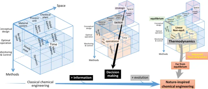
Figure 1 – From classical to nature-inspired chemical engineering: a route across information and evolution
Chen (2016) has sketched an evolution of chemical engineering to bio-inspired chemical engineering considering it as a new branch of chemical engineering due to interaction with biological sciences. But this remains a macroscopic and limited perspective. Here, we discuss more fundamental aspects and we claim that a more theoretical thermodynamic perspective is an interesting way to understand the fundamental underlying mechanisms and to shift chemical engineering toward NICE along a trajectory sketched in Figure 1, using model-driven and enterprise modelling multilevel concepts.
On the left, the 3 × 3 × 3 cube displays an approximate but effective discretization of the chemical engineering domain in three directions. Here, chemical engineering systems can be split over space (+30° axis) into material system, process unit and chemical plant levels. This picture could be further refined by splitting each level into element, mesoscale and system scales (Li et al., 2016): a factory is composed of process unit elements where unit operations happen; and is ran within an environment when addressing the system scale. The mesoscale problem at the plant factory level concerns the process synthesis and requires dealing preliminarily with unit operations. Hence, for solving it, global steady state balances are usually considered while microscopic balances, including non-steady states balances are used to investigate unit operation of process units. In terms of methods (downward vertical axis) and time (-30° axis), a chemical engineer traditionally first carries out a time independent conceptual design stage (check thermodynamic, assess feasibility with simple models, scale-up, elaborate flowsheet, …). He then looks for steady state operating conditions for a cost-optimal operation (refining thermodynamic modelling, simulating with rigorous models, undertaking experiments, etc.) and he goes on with monitoring and control, usually for short term dynamics (start and stop periods, process regulation with linear control theory, etc.).
The middle picture adds the issue of handling information. Already, data is information and feeds chemical engineering everywhere in the left cube representation. Here, the middle picture focuses on the decision making process that integrates information further from an enterprise viewpoint. At the strategic decision level, an extra level must be accounted for, concerning supply chain. Tactical decisions usually concern chemical plants and process unit operation during the design stage. Operational decisions are pertaining to material systems and process units during the optimal operation step as well as to monitoring and control steps.
Supply chain Optimal operation Conceptual design Monitoring & Control Methods Time Process unit Chemical plant Material system Space Optimal operation Conceptual design Monitoring & Control Space Methods Time Process unit Chemical plant Material system Supply chain Optimal operation Conceptual design Monitoring & Control Space Methods Process unit Chemical plant Material system Time Classical chemical engineering + information Nature-inspired chemical engineering + evolution equilibrium Linear Non-equil. Far from equilibrium Thermodynamics strategic tactical operational Decision making Advanced Thermodynamics
4
The right picture maps some thermodynamics concepts over the chemical engineering multiscale and multilevel representation. First, one finds the common phase equilibrium assumption in material systems and process unit models; while dissipative transport phenomena in unit operation models are described with linear phenomenological laws in balance expressions.
When taking into account information, the processing of matter and energy carried out in chemical engineering covers areas similar to what Nature processes. So what is missing to promote NICE? Being inspired by Nature helps clarify the limits of today’s chemical engineering and raises several questions: should we refrain our processes to run in near equilibrium conditions where linear transport law and linear control are used? Is the local equilibrium hypothesis of thermodynamics still valid in nano and microscale processes? What means efficiency for nature and for chemical engineering? Could a novel production organization be inspired by nature?
Within a NET perspective, the notion of evolution covers most of these questions that we complete later. To fulfil precise goals mostly related to survival, natural systems operate near or far from thermodynamic equilibrium, maintain a quasi-steady near-critical state, in an agile way, being adaptable to changes in their surroundings by using efficient strategies of adaptation and adaptability with nonlinear responses and synergies with other nearby systems. These issues are covered in the framework now presented.
3 Nonequilibrium thermodynamics mechanisms for
nature-inspired chemical engineering processes
Chemical engineering and thermodynamics share a long history together and are inseparable. However, thermodynamics is full of misconceptions (Martyushev, 2013; Bejan, 2017, 2018) that one should be aware of especially when invoking the entropy-related notions (second law, disorder, entropy production extremum, …). Entropy is indeed the core concept of thermodynamics. However, the connection between entropy and chemical engineering processes is nowadays overshadowed by two more pragmatic concepts, namely the thermodynamic equilibrium assumption and the use of Fick, Fourier, Newton transport phenomena laws in mass balances. The first is merely a formulation of the second law for isolated closed systems and the second refers to linearized NET equations. But, as highlighted in Figure 2, much more exists in the NET and CL framework, in particular thermodynamic coupling, stationary states, dissipative structure, spatial organization and nonlinear dynamics, that cover partially the three mechanisms T1 T2 T3 already published (Coppens, 2012).
5
3.1 Local thermodynamic equilibrium postulate
The spatial discretization of micro, meso and macro systems in chemical engineering (Figure 1) can be paralleled with the classical thermodynamics assumption that an elemental volume contains enough molecules for microscopic fluctuations to be negligible. This local thermodynamic equilibrium postulate establishes the familiar Boltzmann-Gibbs statistical definition of entropy S for a system of N discernible particles distributed with probability distribution p = {p1, p2, …, pn} among n independent
microstates
𝑆 = −𝑘B∑𝑛𝑖=1𝑝𝑖ln𝑝𝑖 (1)
The average equation above relates the entropy to the probability of occurrence of the possible states of the system, each described by an information content ln(𝑝𝑖).
Nevertheless, the local equilibrium postulate holds no longer in several systems encountered in chemical engineering, where boundaries, fluctuations, configurations and memory effects may impact the definition of local variables (Jou et al., 2010). One can recall that some of the works assigned to the “Force balancing (T2)” mechanisms in nature-inspired engineering evoked by Coppens (2012) discuss the impact of geometrical confinement features of the same magnitude as the molecule size: they may enhance enzymatic activity (Sang and Coppens, 2011; Sang et al., 2011) or provide opportunities for the formulation and controlled release of biological agents (Siefker et al., 2014). Such a confinement brings about local fluctuation and boundary effects that may violate the local thermodynamic equilibrium hypothesis encouraging us to use advanced thermodynamic formalism for improving modelling and understanding (see section 4.1).
3.2 The second law of thermodynamics and thermodynamic equilibrium
Consider a system described by macroscopic variables and undergoing a change along some path. The related entropy S change is the sum of an external contribution dSe due to the interaction of a system
with its surroundings and an internal contribution dSi:
𝑑𝑆 = 𝑑𝑆e+ 𝑑𝑆i (2)
The second law of thermodynamics states that the internal entropy 𝑆i can only increase along an
irreversible path or remains equal for a reversible trajectory, 𝑑𝑆i≥ 0. A consequence well-known
among engineers is that heat flows from high to low temperature regions. Another one is the so-called
MaxEnt principle, namely that the entropy of isolated systems (neither matter nor heat exchange, so
𝑑𝑆e= 0) increases until it reaches a maximum 𝑆equil∗ that is stable {𝛿𝑆 = 𝑆i− 𝑆equil∗ = 0 & 𝛿2𝑆 <
0}. This defines the so-called macroscopic thermodynamic equilibrium.
Using the Lagrange maximisation principle under constant variables constraints over the statistical definition of entropy (equation (1)), MaxEnt translates readily into familiar minimum principles for Gibbs free energy G and Helmholtz free energy F at equilibrium:
{ max 𝑀𝑎𝑥𝐸𝑛𝑡𝑆i} ⇔ { fixed 𝑁, 𝑃, 𝑇 max (−𝐺 𝑇) 𝑜𝑟 min(𝐺) 𝑜𝑟 𝑑(𝐺) = −𝑇𝑑𝑆i≤ 0 fixed 𝑁, 𝑃, 𝑇 max (−𝐹 𝑇) 𝑜𝑟 min(𝐹) 𝑜𝑟 𝑑(𝐺𝐹) = −𝑇𝑑𝑆i≤ 0 } (3)
For open systems 𝑑𝑆e≠ 0 and the system evolution will not be toward an equilibrium state but toward
another state, like a stationary state or a self-organized critical and dissipative state. While Se evolution
can be either positive or negative, the drivers of the positive evolution of Si for an open system are
better captured by Gibbs relation. For a multicomponent system under the local equilibrium hypothesis, it is written as
𝑑𝑆i= (𝑇1) 𝑑𝑈 + (𝑃𝑇) 𝑑𝑉 + ∑ ( −𝜇𝑗
𝑇 ) 𝑑𝑁𝑗
6
3.3 Mass, energy and momentum balances
Equation (4) shows that Si changes as a sum of irreversible contributions from transport phenomena of
internal energy / heat (dU), total mass (dV), component (dNj). To make explicit fluxes of heat and
matter and reaction rates, one must use mass, energy and momentum balances for continuous system, which are more easily expressed with local microscopic specific (per unit mass) variables, for example
e defined as 𝐸 = ∫ 𝜌𝑒𝑑𝑉𝑉 (Bird et al., 2006): 𝜕(𝜌𝑗) 𝜕𝑡 = −𝛻 ⋅ (𝜌𝑗𝐯) − 𝛻 ⋅ 𝐣𝑗+ 𝑀𝑗∑ 𝜐𝑙 j,𝑙𝐽r,𝑙 (mass) 𝜕(𝜌𝐯) 𝜕𝑡 = −𝛻 ⋅ (𝜌𝐯𝐯) − 𝛻𝑃 − 𝛻 ⋅ 𝛕 + 𝜌𝐅 (momentum) 𝜕(𝜌𝑒) 𝜕𝑡 = −𝛻 ⋅ (𝜌𝑒𝐯) − 𝛻 ⋅ (𝐉𝑢+ ∑ 𝑒𝑗 p𝑗𝐣𝑗+ (𝑃𝛅 + 𝛕) ⋅ 𝐯) (total energy) 𝜕(𝜌𝑢) 𝜕𝑡 = −𝛻 ⋅ (𝜌𝑢𝐯) − 𝛻 ⋅ 𝐉𝑢− 𝑃(𝛻 ⋅ 𝐯) − 𝛕: (𝛻𝐯) + ∑ 𝐣𝑗 𝑗⋅ 𝐅𝑗 (internal energy) (5)
Here j and Mj are the mass density and molar mass of component j, 𝐽r,𝑙 is the l reaction rate, 𝛅 is the
unit tensor, P is the pressure and 𝐅 = 1 𝜌⁄ ∑ 𝜌𝑗𝐅𝑗 𝑗
= − 1 𝜌⁄ ∑ 𝜌𝑗𝛻𝑒p𝑗 𝑗
is the mass force with 𝐅𝑗 the
force exerted per unit mass, derived from the component potential energy, for example due to gravitation and intermolecular interactions. 𝐉𝑢= 𝐉𝑞+ ∑ 𝑢𝑗𝐣𝑗
𝑗 with 𝐉𝑞 the pure heat conduction flow
and 𝑢𝑗 the component internal energy transported by the diffusion flow. Other notations are described
below. The first term on the right hand side expressed as a divergence is the convection flow while the remaining terms are conduction flows, contributions of various forces and dissipative terms. The viscous contribution associated with the shear stress tensor 𝝉 and velocity 𝐯 appears in the momentum balance but also in the internal energy balance since 𝑢 is obtained from the total energy balance
𝑒 = 𝑢 + 1 2⁄ 𝐯. 𝐯 + 𝑒p, which necessitates to compute the specific kinetic energy 1 2⁄ 𝐯. 𝐯 and solve
the momentum balance.
3.4 Entropy balance and entropy production equation
The entropy balance for the specific entropy s is analogous to the above expressions but is non conservative and contains an entropy source term :
𝜕(𝜌𝑠)
𝜕𝑡 = −𝛻 ⋅ (𝜌𝑠𝐯) − 𝛻 ⋅ 𝐉s+ 𝜎 (entropy) (6)
The conduction entropy flow 𝐉s has contributions from the heat conduction flow of the internal energy
𝐉u and from the specific diffusion flowjj(Bird et al., 2006). The entropy source term, or local entropy
production per unit volume, 𝜎 is related to the macroscopic internal entropy by the volume integral 𝑑𝑆i⁄𝑑𝑡= ∫ 𝜎𝑑𝑉𝑉 . According to the second law 𝜎 ≥ 0.
Disorganization (rather than disorder) is commonly associated with entropy. But Martyushev (2013) pointed out that the popular axiom “entropy quantity is related to order quantity” is false because it refers only to the system spatial coordinates, discarding momentum contributions and interactions within elements of the system that may also contribute significantly to organization. Equation (6) only establishes that entropy decrease, 𝜕(𝜌𝑠) 𝜕𝑡⁄ < 0, will only happen in a unit volume if the joint contribution of convection −𝛻 ⋅ (𝜌𝑠𝐯) and conduction −𝛻 ⋅ 𝐉s entropy flows are negative and exceed
. But as the total entropy of the system plus surroundings must increase in agreement with the second law, when the internal entropy decreases and results in more organization, the unit volume exports entropy. Freezing a liquid is a typical example as entropy decreases while the system becomes solid and heat is released to the surrounding.
7
The entropy source term 𝜎 is computed from equation (4) by inserting the irreversible contributions arising in the set of transport balances equations (5).
𝜎 = 𝐉u⋅ 𝛻 ( 1 𝑇) + 1 𝑇∑ 𝐣𝑗⋅ [𝐅𝑗− 𝑇𝛻 ( 𝜇𝑗 𝑇)] 𝑗 −1 𝑇𝝉: (𝛻𝐯) + 1 𝑇∑ 𝐴𝑙 𝑙𝐽r,𝑙 ≥ 0 (7) 𝛷 = 𝑇𝜎 = −𝐉u⋅ 𝛻(ln𝑇) + ∑ 𝐣𝑗⋅ [𝐅𝑗− 𝑇𝛻 ( 𝜇𝑗 𝑇)] 𝑗 − 𝝉: (𝛻𝐯) + ∑ 𝐴𝑙 𝑙𝐽r,𝑙 ≥ 0 (8) where 𝐴𝑙 = − ∑ 𝜈𝑗,𝑙𝜇𝑗 𝑗 is the affinity, 𝜈𝑗,𝑙
is the stoichiometric coefficient of species j in reaction l. 𝜈𝑗,𝑙 is positive for products and negative for reactants. Equation (8) is the dissipation function (Demirel
and Sandler, 2004). Equation (7) collects contributions from heat transfer, mass transfer, viscous dissipation of fluid and chemical reactions. Recalling Gibbs relation, Equation (4), it shows a key concept of NET, namely that 𝜎 is a sum of the products of conjugate flows 𝐽𝑘 of extensive variables
𝑈, 𝑉, 𝑁𝑗, 𝑒𝑡𝑐 and forces 𝑋𝑘 of intensive variables, 𝑇, 𝑃, 𝜇𝑗, 𝑒𝑡𝑐 :
𝜎 = ∑ 𝐽𝑘 𝑘𝑋𝑘 ≥ 0 (9)
3.5 Linear nonequilibrium thermodynamics
Equation (9) helps identify the independent flows and thermodynamic forces to be used in the phenomenological equations. Thermodynamic forces are understood as the driving forces of transport and reaction phenomena. Near equilibrium, one can use the linear NET postulates:
1. Thermodynamic forces are not too large.
2. All flows in the system are a linear function of all the forces involved.
𝐽𝑘 = ∑ 𝐿𝑚 𝑚𝑘𝑋𝑚 (10)
3. The matrix Lmkis symmetric provided that 𝐽𝑘 and 𝑋𝑘 are identified by Equation (9).
4. In an isotropic system, the Curie-Prigogine theorem restricts coupling between flows and forces whose tensorial order differs by an even number. However, in an anisotropic medium, all couplings are possible.
The familiar phenomenological laws with positive transport coefficient for heat transfer, Fourrier’s law 𝐉q = −𝑘e𝛻𝑇 = 𝑘e𝑇2𝛻(1 𝑇⁄ ), diffusion, Fick’s law 𝐣𝑗= −𝐷e𝛻𝑐𝑗= 𝐷𝑒𝑐𝑗(−𝜕𝑐𝑗⁄𝜕𝜇𝑗)𝛻(−𝜇𝑗⁄ ), 𝑇
or momentum transfer, Newton’s law 𝝉 = −𝜇𝛻𝐯 obey equation (10). Introduced into each set of conjugate flow and force product of equation (7), one finds immediately that each set is proportional to the square of the thermodynamic force, respectively 𝛻(1 𝑇⁄ ), 𝛻(−𝜇𝑗⁄ ) and 𝛻𝐯. Therefore, the 𝑇 coefficients in the form 𝐿𝑖𝑖 must be positive to ensure that the entropy production 𝜎 is positive. While
Fick’s, Fourier’s and Newton’s laws exhibit a linear dependency on a single thermodynamic driving force only, there are other cases to consider as well. For example Cahn-Hilliard or Guyer– Krumhansl’s models for heat conduction exhibit nonlinear terms (Kovacs and Van, 2005, Jou et al., 2010). Furthermore, equation (10) states that all forces should be concerned when calculating any dissipative flux, which is not the case with Fick’s, Fourier’s and Newton’s laws. This multivariable dependency is called thermodynamic coupling. Curie-Prigogine’s theorem restricts coupling in isotropic media between flows and forces of the same tensorial order (like vectorial mass and heat diffusion but unlike scalar reaction phenomena and vectorial diffusion).
Nature is exploiting coupling at a grand scale. For example, electro-osmosis is responsible for epithelial fluid transport in the corneal endothelium (Fischbarg et al., 2017). Coupling is also considered as a key mechanism behind the RNA world hypothesis for the origin of life, because it explains the accumulation of nucleotides and DNA molecules in hydrothermal pores (Baaske et al., 2007).
8
Table 1. Direct and coupled transport phenomena (Demirel and Gerbaud, 2019, reprinted with permission from Elsevier)
Some couplings are summarized in Table 1. While they have been identified experimentally more than a century ago, only a few chemical engineering processes fully consider them, like in membrane transport when osmotic pressure due to concentration gradient counterbalances hydrostatic pressure (Hwang, 2004); or like in thermodiffusion when ordinary diffusion (−𝐷e𝛻𝑐) counterbalances thermal
diffusion flow (−𝑐𝐷T𝛻𝑇) affecting the volatile composition distribution in oil reservoirs (Faissat et al.,
1994). For polystyrene fractionation, the Soret coefficient 𝑠𝑜𝑟𝑒𝑡 = 𝐷T⁄𝐷e for dilute solutions of
polystyrene in tetrahydrofuran is around 0.6/K, despite small value of the thermodiffusion coefficient, DT =
1 × 10⁻⁷ cm2.s-1K-1. This indicates that the change of polystyrene concentration per degree is 60%
(Schimpf and Giddings, 1989). The thermal gradient drives solute molecules with larger Soret coefficients from the solutes with smaller Soret coefficients. The degree of coupling 𝑞 = 𝐿𝑘𝑚⁄(𝐿𝑘𝑘𝐿𝑚𝑚)1 2⁄ is a useful dimensionless parameter as well as the energy conversion efficiency
𝜂 = output input⁄ for analysing coupled processes (Demirel and Sandler, 2002a).
This balancing of phenomena brings the opportunity to mention “Force balancing (T2)”, the second theme in nature-inspired engineering evoked by Coppens (2012). However, T2 seems different and rather invokes balance between confinement and physical forces (CfNIE, 2019). Out of the twelve T2-related works available at CFNIE website, only one of them (Liu et al., 2009) actually mentions force
balance, when referring to the Maxwell-Stefan approach to model self-diffusion on zeolites, but does
so in a simple way. It states that Fick’s law invoked in the Maxwell-Stefan model is the balance between the driving force for diffusion (i.e., the gradient of chemical potential) and the forces resulting from friction with other species as they interdiffuse.
There are likely some opportunities in exploiting more systematically thermodynamic coupling in chemical engineering, both in steady state and in dynamic operation. In this way, reaction-mass transport coupling between the chemical reactions and the transport of substances in bioenergetics are exemplary as they enable facilitated and active transport of substrates and products across cells membranes (Demirel and Sandler, 2002b).
3.6 Thermodynamic efficiency
At the unit operation scale, thermodynamic efficiency can help define design and operating parameters that minimize irreversibility – entropy production. Whereas infinitely slow reversible operation is not desirable, minimizing irreversibility can be sought (Andresen, 2011). For example, in distillation under optimal operating conditions agreeing with cost and energy optimum (Gerbaud et al., 2019), the column temperature profile is usually increasing smoothly from top to bottom without sharp bend. This agrees with two criteria derived from linear NET when all thermodynamic forces are monitored,
9
either the principle of equal thermodynamic distance (Sauar, et al., 2001), or the principle of equipartition of forces which minimizes the entropy production (Tondeur and Kvaalen, 1987, Kjelstrup et al., 1998). Both indicate that optimal operation is achieved by distributing thermodynamic force gradients, yii T for distillation columns, evenly across the apparatus, which results in small
temperature steps from tray to tray (Sauar, et al., 2001). Similarly, one should have a uniform Gibbs energy of reactionrG T for chemical reactors (Sauar et al., 1997) and a uniform T T for heat exchangers, which happens more readily in countercurrent than in concurrent heat exchangers (Tondeur, 1990). When some forces are not controlled, “the EoEP, but also EoF are good approximations to the state of minimum entropy production in the parts of an optimally controlled system that have sufficient freedom” and is not too far from equilibrium (Johannessen and Kjelstrup, 2005).
The equipartition principle has been used in one of the cases illustrative of the T1 mechanism – hierarchical transport network (Coppens, 2012) by Kjelstrup et al. (2010) for designing a new fractal gas supply system for a polymer electrolyte membrane (PEM) fuel cell inspired from human lung. The gas supply system in a PEM fuel cell works as follows: (a) a single gas stream is distributed to the entire surface of the cell, and (b) the transport mechanisms changes from convection (inside the flow plates) to diffusion (inside the porous transport layer). Both these features are also observed in human lungs. The novel fractal distributor allows the oxygen to be homogeneously distributed along the cell’s surface. The earlier nanoporous catalytic layer is now replaced by a macroporous/nanoporous layer, and macroporosity distribution is constrained to ensure uniform entropy production and minimize total entropy production. One should then expect that it will be optimal in some economic sense (Tondeur and Kvaalen, 1987). Indeed, it showed a reduction of 75% in the amount of catalyst required, whilst increasing the energy efficiency by 10-20% (Kjelstrup et al., 2010). In membrane separation, the design of a composite membrane with layers of nanostructured films enables to achieve remarkable solvent permeance and high retention of dissolved solutes (Karan et al., 2015).
Nevertheless, this discussion about thermodynamic efficiency is limited to unit operations within a given design process unit architecture. It does not address the time evolution of the design or of the operation that we now discuss.
3.7 Steady state evolution
Once the full expressions of the dissipative fluxes are explicated in terms of all forces according equation (10), they are inserted into the partial differential balances (equation (5)) which are solved along with boundary conditions to obtain all state variables time and space evolution. Indeed, chemical processes are time dependent and it is worthy to decipher what evolution means in thermodynamics. For a macroscopic isolated closed system, the second law states that it evolves toward thermodynamic equilibrium (left side of Figure 2). Done in a reversible way, it requires an infinite time, which implies that power, as the ratio of work over time, is null. So irreversibility must be assumed in processes to do some work, hammering the shortcut thinking that process improvement, in particular regarding energy consumption, must go through a thermodynamically reversible operation.
For open systems, evolution will not achieve thermodynamic equilibrium but could well reach a stationary state (right side of Figure 2) which obeys the following relation:
{𝑑𝑆𝑑𝑡 =𝑑𝑆e 𝑑𝑡 + 𝑑𝑆i 𝑑𝑡 = 0} ⇔ { 𝑑𝑆e 𝑑𝑡 < 0 since 𝑑𝑆i 𝑑𝑡 > 0} (11)
As internal entropy must increase, reaching a stationary state requires that the system is not isolated and entropy exchanged with the surrounding is negative, implying a balancing between external (e.g. heat) and internal (equation (7)) entropy contributions to the total entropy. One could take advantage of thermodynamic coupling (section 3.5): in the Soret effect, a temperature gradient imposed from outside may counterbalance the diffusion flux inside the system.
10
3.8 Dynamic evolution
The third and last theme for nature-inspired engineering proposed by Coppens (2012) is T3 – Dynamic Self-Organization. Continuous manufactories are generally designed for steady-state operation, and fluctuations are seen as anomalies that need to be “controlled”. However, this “stationary” way of thinking, common in process engineering, has deprived engineers from fully exploring the time dimension in the design of unit operations and processes, which Coppens’ proposal with T3 mechanism encourages somehow. More specifically, theme T3 draws inspiration from organized, natural structures that appear as a result of intermittent stimuli from their surroundings. The classical example is that of sand waves. Sand waves (the organized structure) are formed through oscillatory wind tides (the intermittent stimulus). Inspired by this phenomenon, Coppens and van Ommen (2003) proposed the use of oscillating gas flow in fluidized beds. They found that oscillating the gas inlet flowrate (the intermittent stimulus) creates a regular bubble pattern (the organized structure) at the lower part of the bed. This helps increasing control over the otherwise chaotic hydrodynamics of the bed. Furthermore, it prevents channelling and clumping, improving processes such as combustion and drying (Coppens, 2012). Another example is related to mixing operation. Compared to the stirred tank reactor, the soft elastic reactor inspired by the animal upper digestion track improves mixing, inducing it by periodic wall deformations triggered by a peristaltic movement (Liu et al., 2018).
3.8.1 Fluctuation theorems, irreversibility and second law
Introduced by Evans and Searles, fluctuation theorems (FT) are numerous (transient FT, integral FT, detailed FT, …) (Mittag et al., 2007). Here, they help clarify the notion of reversibility and the second law statement. Consider an evolution trajectory between two states and its entropy production quantity, with a time distribution and a time-average value over interval 𝜏 > 0, 𝜎̅𝜏. A fluctuation
relation examines the symmetry of 𝜎̅𝜏 around its value a = 0, and compares the probability of the
forward path 𝑝F(𝜎̅𝜏= +𝑎) with that of the reverse path 𝑝R(𝜎̅𝜏= −𝑎). Among FT, Crooks’ relation
states for systems in which the relaxed initial and final states have the same free energy, that
𝑝F(𝜎̅𝜏=+𝑎)
𝑝R(𝜎̅𝜏=−𝑎)= 𝑒
𝑎𝜏 (12)
Two remarks are worth mentioning. First, both extensive entropy production and path time interval τ
are small for a microscopic system, so the exponential limit goes to unity, exemplifying microscopic time reversibility as 𝑝F= 𝑝R. Equation (12) hints that the same ratio 𝑝F/𝑝R can be obtained when 𝑎𝜏
is constant. But for a reversible path (𝜎̅𝜏= 0) reaching the final state requires an infinite time. So, for
large system, irreversible evolution is unavoidable and welcome. It will make the probability ratio in equation (12) greater than unity, thus enabling the system to effectively reach the final state. Secondly, analyzing the average 〈. . . 〉 over many paths along the evolution trajectory, equation (12) is analogous to 〈𝜎̅𝜏〉 ≥ 0 (Demirel and Gerbaud, 2019). This is a statement of the second law, demonstrating that
the second law is valid on average. This implies that there can exist some paths with negative internal entropy production, while on average the entropy production is positive.
3.8.2 Constructal law
Whereas thermodynamics deciphers the phenomenological mechanisms, the CL is a principle of design, resulting in how will evolve the organization, architecture and structure for living and nonliving systems in nature (Bejan and Lorente, 2013; Bejan, 2017). CL is about survival by increasing efficiency, territory and compactness (Bejan and Lorente, 2004). Considering a global flow resistance (opposite of performance) R, the global internal size V, and global external size (covered territory) L, survival is achieved depending on what is fixed:
R minimum at constant L and V ⇔ easiest flow access
V minimum at constant R and L ⇔ compactness or more free space L maximum at constant V and R ⇔ maximal spreading
11
Equation (13) shows the importance of the CL to engineers. Indeed, the three features at the right-side of the arrows (easiest flow access, compactness or more free space, maximal spreading) are the drivers for the conception of transport networks. When designing the pipe network for a chemical plant, engineers want to minimize the pressure drop (i.e., the resistance to the flow) in order to lower the cost of pumping. However, transport of corrosive fluids requires expensive materials, such as titanium or zirconium alloys. In those cases, engineers may prefer to minimize the capital cost of construction (i.e., minimize the material used for transport) by accepting a fixed maximum pressure drop. This is similar to the second principle listed in equation (13). Finally, road networks are conceived to connect the different parts of a city. The optimal configuration in this case is the one covering the maximum territory available, following the third principle in equation (13).
The fractal gas supply distributor in the PEM cell (Kjelstrup et al., 2010) evoked earlier in Section 3.6 is one of the illustrative cases of T1 mechanisms Hierarchical transport network (Coppens, 2012). It displays some fractal-like geometrical features alike those derived from the CL (Bejan and Tondeur, 1998). Performance of such hierarchical fuel cells are greatly improved in terms of increased current density, maximum power density, lower pressure drop (Trogadas et al., 2018). Fractal tree structures emerge from CL, when it is necessary to connect one point with an infinite number of points covering a surface/volume. Fractal structure also facilitates scale-up. Two examples are the vascular and the respiratory networks in the human body. Tree-shaped networks are also found to dissipate energy uniformly (West et al., 1997) and to operate near optimality in terms of momentum and heat flow resistance (Bejan and Tondeur, 1998, Coppens, 2012). This feature illustrates some connection of both the CL and T1 mechanism with the principle of equipartition of entropy production that was already evidenced by Coppens (2012). Along its evolution, Nature has promoted such transport network which favors its survival and minimizes irreversibilities. It should be a source of inspiration for engineers.
3.8.3 Minimum and maximum entropy production
Taking a broader perspective of a system evolution, the NET community has debated about two principles: minimisation of entropy production (minEP) and maximisation of entropy production (maxEP) which are encompassed by Ziegler’s maximisation entropy production principle (Martyushev, 2013).
Historically, minEP was derived by Prigogine for systems near equilibrium where linear phenomenological equation (10) applies and some forces are kept constant (Moroz, 2011, Kondeputi and Prigogine, 2014). Then, the entropy production is a quadratic definite expression: 𝑑𝑆i⁄𝑑𝑡=
∫ 𝜎𝑑𝑉𝑉 = ∫ ∑𝑚,𝑘𝐿𝑚𝑘𝑋𝑚𝑋𝑘𝑑𝑉 𝑉
. Prigogine established that if a system has n independent forces (𝑋1, 𝑋2, … , 𝑋𝑛), and j of them are held constant (𝑋1, 𝑋2, … , 𝑋𝑗= 𝑐𝑜𝑛𝑠𝑡𝑎𝑛𝑡), then the other flows
𝐽𝑗+1, 𝐽𝑗+2, … , 𝐽𝑛= 0 at the stationary state with minimum entropy production represented by
{(𝑋𝑘 fixed (𝑘 = 1, … , 𝑗)) min𝐸𝑃 = min𝑋𝑗+1,…,𝑋𝑛(𝑑𝑆i⁄ )𝑑𝑡 } (14)
The so-called maximum entropy production principle (maxEP) proposed by Ziegler has a broader reach, including far from equilibrium where linear phenomenological laws may no longer be valid (Martyushev and Seleznev, 2006). This principle states that for given forces, the system sets the fluxes in order to maximize entropy production. Despite being generally well-accepted in academia, there is still a debate on its application beyond linear regime for some systems in particular for compound systems with independent parts (Polettini, 2013; Martyushev and Seleznev, 2014).
{(𝑋𝑘 given (𝑘 = 1, … , 𝑛)) max𝐸𝑃 = max
𝐽 (𝑑𝑆i⁄ )} 𝑑𝑡 (15)
In a unifying perspective, minEP principle is also shown to be related to Ziegler’s maxEP principle (Moroz, 2011). Quoting Martyushev (2013), physical and biological system evolutions comply with both principles: “for small times, the system maximizes the entropy production with the fixed forces
12
time, the system varies the free thermodynamic forces in order to reduce the entropy production”.
Moroz (2008) interpretation is similar as over time entropy production is minimal but it proceeds as fast as possible by maximizing the energy dissipation rate. Li et al. (2016) pictured this temporal sequence as a compromise between mechanisms that may dominate under different operating regimes and could be formulated as a multiobjective variational problem (Li et al., 2018).
maxEP has also led Prigogine to introduce the concept of dissipative structure often associated with self-organized criticality (SOC). The SOC concept is a strong driver for nature-inspired processes because evidences exist that many natural systems lie in a SOC state (Bak, 1996). Dissipative structures are far from equilibrium and energy-sustained states which existence can be justified as states that enable (often in a nonlinear way) a faster dissipation (maxEP) than would linear mechanisms occurring near equilibrium. For open-system they may last as long as energy flows in while for closed sytem they last for a limited time along the path toward thermodynamic equilibrium (Moroz, 2008). Submitted to external changes in their surroundings, they will evolve in an unpredictable manner, either shifting to another SOC state with different organization, undergoing cyclic evolution around the critical SOC state following so-called punctuated equilibrium evolution, or something else. Properties of SOC are debated but one agrees that an initial fluctuation becomes amplified until criticality is reached and that some phenomena follow a power law distribution: size vs frequency, duration and amplitude of punctuated equilibria, etc, which leads to scaling (Pruessner, 2012).
Many phenomena considered as SOC have been described with the help of thermodynamics principles minEP and maxEP depending on which constraints are holding (Dewar et al., 2014). Out of the linear region, there exists a generalization of the maxEP principle (Martyushev and Seleznev, 2006). In particular, for slowly-driven flux systems, maxEP principle has been proposed as the thermodynamic driver for the emergence of SOC (Dewar et al., 2014, Dewar and Maritan, 2014). Benard cells are an example of SOC not far from equilibrium: convection cells appear in a heated liquid over some critical threshold of external heating. Compared to heat conduction, convection is then more efficient for dissipating in the fastest way the heat provided, and entropy production is maximal.
{(slowly-driven flux 𝐽𝑘 ) max𝐸𝑃 = max(𝑑𝑆i⁄ )} 𝑑𝑡 (16)
While discussing T1 mechanism (hierarchical transport network), Coppens (2012) has mentioned that diffusion-dominant transport networks are usually uniform and non-scaling. As convection becomes dominant, scaling like fractal structure may occur, which is also a feature attributed to SOC as discussed above. Li et al. (2018) further added reaction as a mechanism leading to clustering. This recognized feature has been used to design hierarchically structured catalyst where nanoporous grains not limited locally by diffusion are dispersed into a macropore network of optimized uniform porosity (Trogadas et al., 2016a, 2016b, Hartmann and Schwieger, 2016). The emergence of dynamic heterogeneity in several chemical engineering applications has been postulated to be caused by a compromise in competition between mechanisms that are driven either by minEP or maxEP principles (Li et al., 2018).
SOC are discussed in many scientific domains: engineering, biology, climatology, economics, social sciences. One aspect of SOC lies in their presupposed adaptability to changes in their environment. Some have recognized that their evolution is unpredictable but follows irregular cyclic successions of so-called punctuated equilibria, alternation of fast and slow response to external stimuli. The theory was proposed in evolutionary biology (Gould and Eldredge, 1977, Bak, 1996).
Appealing as it seems in terms of robust operation for chemical processes needing to cope with increasingly variable inputs or outputs nowadays, the SOC state evolution likely requires appropriate controls far from equilibrium.
13
3.8.4 Nonlinearity vs. controllability
Even if the dissipative fluxes (equation (10)) are linear with respect to the thermodynamic forces, the partial differential balance equations (5) for the state variables may exhibit nonlinearities (e.g. due to convection terms). By integrating over the entire system, nonlinearity might also emerge. In chemical engineering, control systems are used to ensure the stability of the prescribed process regime, typically, a steady-state regime. For this purpose, a linear approximation of the nonlinear process in terms of deviations from the targeted regime is sufficient to model the process behaviour. However, far from the equilibrium or from a stationary state of the system, the linear approximation of the nonlinear macroscopic balances may no longer be valid. This makes impossible the analysis of the dynamics and controllability of the thermodynamic system with classical linear control methods. On the other hand, criteria of controllability, observability and optimality of nonlinear dynamical systems, originally introduced for the purpose of control of artificial automated systems, can be successfully applied to the analysis of natural systems like minimal time control problem for fed-batch bioreactors (Bayen and Mairet, 2013) or finding optimal intervention strategy to epidemics (Sharomi and Malik, 2017), or other systems exploiting nonlinear phenomena.
In this section, we assume that the behaviour of a thermodynamic system can be described by a system of ordinary differential equations of the general form
𝑑𝒙
𝑑 𝑡= 𝒇(𝒙, 𝒘) (17)
where 𝒙 ∈ 𝑀 is a vector of state variables of the systems belonging to the state space manifold 𝑀 and 𝒘 ∈ 𝛺 ⊂ ℝ𝑚, 𝑚 ≤ dim 𝑀, denotes the vector of control parameters. The vector function 𝒇(𝒙, 𝒘) ∈ 𝛺 describes the set of generalized flows of the systems. We further assume that it is sufficiently smooth to verify all the theoretical results discussed below. In the case of distributed systems, the state vector 𝒙 contains the momenta associated to the distributed variables via their convolution with the density distribution function, for instance, in the case of hydrodynamics, density, momentum density and entropy density (Grmela, 2015).
The system (17) is said to be controllable if any given pair of initial and final states 𝒙0 and 𝒙f can be
steered by its trajectory by an appropriate choice of control 𝒘(𝑡). Near equilibrium, the behaviour of the nonlinear systems is well approximated by the linear system of the form 𝑑𝒙/𝑑𝑡 = 𝐴𝒙 + 𝐵𝒘 and the famous Kalman controllability criterion provides the necessary and sufficient condition of controllability of a linear system:
𝑟𝑎𝑛𝑘[𝐵: 𝐴 𝐵: … 𝐴𝑛−1𝐵] = 𝑛 (18)
Without loss of generality, we may rewrite general equation (17) as an affine control system of the form:
𝑑𝒙
𝑑𝑡 = 𝒇0(𝒙) + ∑ 𝑤𝑘 𝒇𝑘(𝒙) 𝑚
𝑘=1 (19)
with piece-wise constant controls. Equation (19) can always be obtained by an appropriate choice of state variables and control parameters. The drift term 𝒇0 (𝒙) describes the natural evolution of the
system in absence of control, while the vector fields 𝒇𝑘 (𝒙) describe the influence of the control
parameter 𝑤𝑘 on the global dynamics of the systems. Then, the controllability analysis of a nonlinear
system (19) relies on the computation of the iterated Lie brackets of the control and drift vector fields1. The Lie bracket 𝐿𝑖𝑒{𝒇, 𝒈} is the Lie derivative of 𝒈 along the flow generated by 𝒇. It measures the commutativity of the flows generated by the vector fields in the state space. In fact, a pair of flows generated by a pair of vector fields commute if and only if their Lie bracket is zero. The Lie algebra of
1
The Lie bracket of pair of the vector fields 𝒇and 𝒈 is a vector field [𝒇, 𝒈] = 𝒇 ∘ 𝒈 − 𝒈 ∘ 𝒇 whose components can be computed as follows: [𝒇, 𝒈]𝑘(𝒙) = ∑ 𝑓𝑗(𝒙)𝜕𝑔𝜕𝑥𝑘
𝑗(𝒙) −
𝑛
𝑗=1 𝑔𝑗(𝒙)𝜕𝑓𝜕𝑥𝑘
14
control system (19) is the vector space generated by the vector fields 𝒇0, … , 𝒇𝑚 together with their
iterated Lie brackets:
𝐿𝑖𝑒{𝒇0, … , 𝒇𝑚} = 𝑠𝑝𝑎𝑛{𝒇0, … , 𝒇𝑚, … , [𝒇𝑖1, [… , [𝒇𝑖𝑘−1, 𝒇𝑖𝑘]]], 𝑖𝑘 ∈ {0, … , 𝑚}, 𝑘 ≥ 1} (20)
The control system (19) is said to verify the Lie Algebra Rank Condition (LARC) if every direction in the state space M can be realized by a vector field 𝒈 ∈ 𝐿𝑖𝑒{𝒇0, … , 𝒇𝑚}, i.e.
𝐿𝑖𝑒{𝒇0, … , 𝒇𝑚}(𝒙) = 𝑇𝒙𝑀 for all 𝒙 ∈ 𝑀 (21)
where 𝑇𝒙𝑀 is the tangent space to the state space manifold M at point 𝒙. The following criteria provide
the controllability conditions (Jurjevic, 1997).
1. In absence of restrictions on the controls, i.e. if 𝛺 = ℝ𝑚, LARC condition (21) is sufficient
for the controllability of nonlinear affine control system (19).
2. If the set of controls is bounded, the driftless system 𝑑𝒙/𝑑𝑡 = ∑𝑚𝑘=1𝑤𝑘 𝒇𝑘(𝒙) verifying the
LARC condition (21) is controllable provided that 0 belongs to the interior part of the control set 𝛺 ⊂ ℝ𝑚.
3. Control system with (19) verifying (21) is controllable if the drift vector field is recurrent, i.e. for all initial conditions and in absence of controls, 𝑑𝒙/𝑑𝑡 = 𝒇0(𝒙) returns arbitrarily close to
its initial state at some time.
LARC’s condition (21) generalizes Kalman’s linear system condition (18) for nonlinear systems, but it is much stronger. Indeed, a linear approximation of a controllable nonlinear system is controllable in the sense of criterion (18), but the opposite is not true. In particular, a nonlinear system evolving far from equilibrium under the influence of large control functions can be controllable even if its linear approximation close to an equilibrium is not.
The typical obstacle to the controllability is the existence of the dynamical invariants of the system, called first integrals. The application of the LARC allows recognizing the existence of such hidden invariants. The following example of a fed-batch bioreactor illustrates this concept. The dynamical model of a bio-reactor with single species is given by the following system of equations (Bayen and Mairet, 2013): 𝑑𝑧 𝑑𝑡 = −𝜇(𝑧)𝑏 + 𝑤 𝑧in−𝑧 𝑉 , 𝑑𝑏 𝑑𝑡 = 𝜇(𝑧)𝑏 − 𝑤 𝑏 𝑉, 𝑑𝑉 𝑑𝑡 = 𝑤 (22)
where 𝑏, 𝑧 are concentrations of biomass and substrate, 𝑉 ∈ [0, 𝑉𝑚𝑎𝑥] is the volume of the tank,
𝑤 ∈ [0, 𝑤𝑚𝑎𝑥] is the controlled input flow rate, 𝑧
in is the substrate concentration in the input flow and
𝜇(𝑧) > 0 is the growth rate function of the bacteria. This system can be written in the affine form
𝑑𝒙
𝑑𝑡 = 𝒇0(𝒙) + 𝑤 𝒇1(𝒙), with 𝒙 of dimension 3 where
𝒇0= (−𝜇(𝑧)𝑏, 𝜇(𝑧)𝑏, 0)𝑇, 𝒇1 = ( 𝑧in−𝑧 𝑉 , − 𝑏 𝑉, 1) 𝑇 , 𝒙 = (𝑧, 𝑏, 𝑉) ∈ ℝ+× ℝ+× [0, 𝑉𝑚𝑎𝑥]. (23)
Starting the iterative Lie bracket computation to find an extra third direction in addition to the already independent directions 𝒇0 and 𝒇1, we get for the first bracket
[𝒇0, 𝒇𝟏] = ( (𝑧in−𝑧) 𝑏 𝜇′(𝑧) 𝑉 , − (𝑧in−𝑧) 𝑏 𝜇′(𝑧) 𝑉 , 0) 𝑇 = −(𝑧in−𝑧) 𝜇′(𝑧) 𝑉𝜇(𝑧) 𝒇0 (24)
In fact, going further with the Lie bracket computation one will always get the drift direction 𝒇0, so
LARC condition (21) is never fulfilled since we cannot get a third direction necessary to span the tangent space 𝑇𝒙𝑀. Indeed, the following quantity 𝐾 = 𝑉(𝑏 + 𝑧 − 𝑧in) is constant and thus invariant
for the evolution of the system (22). This means that the system is not controllable in the original state space whatever is the grow rate function 𝜇(𝑧). By introducing the constant 𝐾, the original problem (22) is reduced to the following one:
𝑑𝑧 𝑑𝑡 = −𝜇(𝑧) ( 𝐾 𝑉− 𝑧 + 𝑧in) + 𝑤 𝑧in−𝑧 𝑉 , 𝑑𝑉 𝑑𝑡 = 𝑤 (25)
15 with 𝒇̃ = (−𝜇(𝑧) (0 𝐾 𝑉− 𝑧 + 𝑧in) , 0) 𝑇, 𝒇 1 ̃ = (𝑧in−𝑧 𝑉 , 1) 𝑇
, when written in the affine form shown in (19). The LARC condition is trivial and satisfied (condition 2 above). Then, since 𝑏 > 0, the reduced system is controllable provided that the growth rate 𝜇(𝑧) verifies certain properties making the vector field 𝒇̃ recurrent (condition 3 above). 0
4 Challenges for nature-inspired chemical engineering
Bearing in mind Coppens’ mechanisms and the NET mechanisms that we have attempted to elucidate, engineers may be able to innovate by questioning the hypothesis behind the models they use, instead of taking them for granted. For instance, we have suggested examining the relevance of classical models for novel systems, to think of thermodynamic coupling, to consider larger flows in the nonlinear regime that would be still safe to operate with appropriate non-linear regulation, and to envision a novel resilient production organization. These are the challenges that we explore in this section.
4.1 Change in the system: examining the local equilibrium hypothesis
The local thermodynamic equilibrium assumption remains valid at remarkable small scales, for example down to 8-18 particles subjected to large temperature gradients (1012 K/m) and mass fluxes (13 kmol/m2s) in homogeneous systems and slightly larger but still small values in porous or interfacial system (Kjelstrup et al, 2008, Schweizer et al., 2016, Kjelstrup et al., 2018). Indeed, a criterion based on the magnitude of local relative fluctuation of state variable has been devised for testing the validity of the local equilibrium hypothesis (Kjelstrup et al. 2008) and if that is true classical NET can be used. But the local thermodynamic equilibrium may be violated in many aspects in some rheological, thermal, polymer applications (systems with non-negligible relaxation times), chemical reactions or non-newtonian fluids (nonlinear phenomenological equations), configuration-dependent systems, micro and mesoscopic-fluctuation-configuration-dependent systems, nanoscale systems, systems with wavelength-dependent phenomenological diffusion, systems with range interactions or long-range microscopic memory, …. Observed state variables are then very different from the bulk one predicted by classical thermodynamics, like the melting point depression for nanoparticles (Letellier et al., 2007), or a time lag of the propagation of heat flow where Fourier linear phenomenological equation predicts that the heat flow is felt instantaneous and everywhere in the system (Lebon and Jou, 2014).
In such cases, new variables related to configuration, fluxes or gradients can be introduced in the thermodynamic equations in addition to classical state variables to account for memory and boundary effects. Many approaches coexist (Demirel and Gerbaud, 2019). One can define a nonequilibrium temperature starting from the equilibrium bulk temperature but dependent on heat flux within the ENET formalism (Jou et al., 2010); incorporate time evolution of mesoscopic dynamics in the GENERIC formalism to analyse dynamic evolution (Öttinger, 2005); take into account local fluctuations with mesoscopic thermodynamics (Rubi, 2008) or re-examine the extensive character of several variables like entropy from either a statistical viewpoint revisiting Boltzmann-Gibbs statistics (Tsallis, 1988, Tsallis et al., 1998) or from a phenomenological approach more suited to chemical reactions (Turmine et al., 2004; Letellier et al., 2015). In these latter works, the effect of confinement is handled by considering geometric boundaries as a fuzzy interface, introducing a non-extensive contribution of the interfacial energy in the internal energy. Internal energy and entropy then become non-extensive de facto. It would be interesting to use such advanced thermodynamics formalism for studying nanoscale confinement effects as in works referred to the Force balancing T2-mechanism (Sang and Coppens, 2011, Sieker, et al., 2014).
16
4.2 Change in the environment: resilience and efficiency
The variability of raw materials is well managed through chemical engineering activities based on fossil fuels. However, there is a concern about the adaptability of processes to the variability and intermittence of renewable material and energy. As chemical engineers become ever more involved in the design and operation of such processes, they face two challenges that resonate with Nature’s remarkable capabilities: efficiency and resilience. Resilience is the ability of a system to overcome changes in its surroundings so as to maintain operation. Efficiency is a master goal in industrial operations. Efficiency is related to resource usage, in particular energy.
In nature, biochemical reaction processes are complex cyclic processes archetypal of processes that must keep functioning, whatever the changes in nutrients, in demand and in environment. Whereas kinetic equations and statistical models can describe such processes satisfactorily, the NET theory can help describe energy pathways and coupling in a quantitative manner and formulate the efficiency of energy conversion in bioenergetics. For example, mitochondria in biological cells respond to the cell energy demand through the production of adenosine triphosphate (ATP) further used in metabolic activities, like synthesizing protein molecules, transporting ions and substrates or producing mechanical work. Thanks to the monitoring of the coupling between ATP production (J ) and oxygen P
consumption (J ), mitochondria maintain a quasi-steady state robust to external and internal changes O
in the cell energy demand (Stucki, 1991). ATP-utilizing reactions act as a load as well as thermodynamic buffers that regulates the process efficiency. This regulatory mechanism based on monitoring the degree of coupling qLPO
L LPP OO
1/ 2allows oxidative phosphorylation to operate with an optimal use of the exergy contained in the nutrients for achieving various objectives: maximize ATP production at optimal efficiency
JP optatq0.786, maximize power output at optimal efficiency
J XP P opt
atq0.91, minimize energy cost for a net ATP production
P
at 0.953opt
J q , or minimize energy cost for net output power
P P
at 0.972opt
J X q (Stucki,
1980; Demirel, 2004).
It is tempting to make a parallel with challenges met at a macroscale level as suggested by Chen (2016) when he compares the biofuel production circular production to a cellular biochemical cycle and calls for improving operational efficiency, scalability and robustness. In a biorefinery, renewable raw material processing requires usually to spend a lot of energy to remove the water in large excess before manufacturing any commodity. In terms of resilience, biorefinery plants must comply with a strong variability of raw material flowrate and compositions and with a market induced variability of output demand as well, while maintaining an efficient operation. In this case, efficiently maximizing production or output power and/or minimizing energy costs are routine objectives. Reasoning at the plant scale may help identify flux and forces whose coupling regulation would help to increase the resilience of the process.
4.3 Distributed production and the management of information
Going a step further, the self-organization critical state embraced by many natural systems advocates for a possible novel organization of chemicals production that would be robust to changes. It is superfluous to claim reaching a SOC state for a plant, but one can think to design a self-organized plant.
Roughly speaking, SOC system adapts to changes by mobilizing fast and strong response when the change is sudden and milder response when it is slow. The way different responses are occurring can be paralleled with the solicitation of alternative mechanisms triggered by thermodynamic coupling in cells in response to cell energy demand changes (Stucki, 1991). In a self-organized plant that would suggest to get access to several mechanisms, by designing several production lines with alternative
17
processes. For obtaining a chemical product, several production pathways may be available. Different pathways will employ different feedstocks, reactions, catalysts, temperatures, pressures, etc. Conversion rates and efficiency will also differ depending on the pathway.
Multiplying the production routes is a way to robustness, but will likely be costly. To improve economic viability, Budzianowksi and Postawa (2016) have proposed the total integration of biorefinery systems by combining platforms using different biomass feedstock and by considering environmental and social issues as well. In the same spirit, the optimization of eco-industrial parks should encourage industrial symbiosis. Chen (2016) has envisioned the large-scale biofuel production from microalgae as a circular production route similar to a biochemical cellular cycle. But, this is so far restricted to material and energy network, lacking a proper formulation of social objectives (Boix et al., 2015).
These biorefinery and eco-industrial proposals call for a tight spatial integration that may fail to provide enough flexibility. A way out is to envision a modular chemical plant, as proposed by the F3 factory modular equipment project (Buchholtz, 2014) that demonstrated how a flexible scalable continuous technology, like standardized process equipment containers, can, for low- and medium-scale productions, achieve reductions in start-up, building and operating costs, in energy consumption, in waste, etc. Material and energy exchange interface should be standardized as well, in the spirit of a physical internet network (Montreuil et al., 2013).
The aforementioned flexibility should also concern automation as well as logistics and supply chain (Weber, 2016). More generally, the self-organized plant should qualify as agile, where agility is defined as encompassing detection, adaptation, responsiveness and efficiency (Barthe-Delanoe et al., 2014). To meet the challenge of handling information in a modular multipurpose multiple feedstocks factory, the next step is the shift from a physical factory integration perspective to a virtual factory perspective. Using a model-driven engineering approach, a metamodel for knowledge management and collaborative process design has been conceived in the case of biorefineries of a novel kind. They are seen as a virtual assembly of data and information, operated with a mediation information system and relevant to stakeholders who provide ‘services’ to meet the flexible demand described as ‘collaborative objectives’ within a ‘context’ about location, weather forecast, consumer, biomass physical property information (Houngbe et al., 2018). This virtual factory approach refers to what is called servitization, already in use regarding business models (Baines et al., 2017), and that must now expand to the chemical plant level: context and demand help generate an ad-hoc production pathway that is materialized as an assembly of blocks providing services. Underlying ontologies help managing the process and information workflow and its governance through the multiple scale hierarchy from the process unit to the industrial plant (Benaben et al., 2016; Zhou et al., 2018). In practice, the mediation information system assesses new collaborative objectives (e.g. change in demand) and context changes (e.g. impure feedstock) to design a novel production line built through the reuse of existing devices (unit operations, energy supplieers, logistical units). A case study is presented in Houngbe et al. (2019).
But how to reach and maintain a self-organized state far from equilibrium, like a SOC system? There is evidently a necessity to refer to what Coppens’ recently called the mechanism T4 (control mechanisms in ecosystems, biological networks and modularity). In our case, this is where nonlinear control comes into picture.
4.4 Nonlinear control
4.4.1 Dynamic state equation far from equilibrium
What if we accept to run a process with large driving forces and fluxes? This might prompt potentially unstable or erratic behaviour leading to failure of the process. In this case, risk monitoring cannot be handled only with linear control theory as the evolution of the system is governed by a full nonlinear