Diagnostic Studies of ECHAM GCMs
by
Ji-yong Wang
Submitted to the Department of Earth, Atmospheric, and Planetary
Sciences in partial fulfillment of the requirements for the degree of
Master of Science in Meteorology
at the
MASSACHUSETTS INSTITUTE OF TECHNOLOGY
September, 1998
@ Massachusetts Institute of Technology, 1998. All Rights Reserved.
A u th or ... ... ...
Department of Earth, At ospheric and Planetary Sciences
August 3, 1998
Certified by ...
Peter H. Stone
Professor
DepartmepmLatthLAtmospheric, and Planetary Sciences
A ccepted by ...
Ronald Prinn
Department Head
Department of Earth, Atmospheric, and Planetary SciencesMASSACHUSETTS INSTITUTE FTECHNOLOGY
Diagnostic Studies of ECHAM GCMs
by
Ji-yong Wang
Submitted to the Department of Earth, Atmospheric, and Planetary Sciences on August 3, 1998, in partial fulfillment of the requirements for the degree of
Master of Science in Meteorology
Abstract
The two latest generations of MPI ECHAM AGCMs, ECHAM3 and ECHAM4, have been performed the test run in relatively high resolution (T106) with the prescribed AMI boundary conditions. There are major changes made in ECAHM4 T106 from ECHAM3
T106 in the radiation scheme, the treatment of radiation absorption by water vapor and
cloud water and the calculation methods of advection of water vapor and cloud water, etc. It is shown that the simulation of annual mean heat balance at ocean surface has been
greatly improved in ECHAM4 T106 with respect to the GEBA observations.
While the annual mean state is important to the global climate system's heat and water balance, the distribution of global heat and water divergence determines the energy and water mass transport in the atmosphere and between the ocean and atmosphere. The diag-nostic studies of ECHAM AGCMs' implied oceanic meridional heat transport and their comparison with available observational data, and the break-down of model annual sur-face heat balance terms highlight the importance of model's treatment in radiation absorp-tion of atmospheric water vapor, the cloud radiaabsorp-tion forcing calculaabsorp-tion and latent heat contribution from hydrological balance requirement.
The ECHAM GCMs' response with the ocean-atmosphere boundary condition is also investigated with MIT's ECHAM4 T42 datasets, which are obtained with the two different boundary conditions. The ECHAM4 model is capable in simulating the annual mean implied oceanic meridional heat transport with fare accuracy in T42 resolution, while the interannual variation is clearly shown.
Thesis Supervisor: Peter H. Stone Title: Professor
Contents
List
of
Tables
...
3
List of Figures
...
4
A cknow ledgm ent ...
9
1
ntroduct1
n ...
10
1.1 Background ...
10
1.2 M otivation ...
13
1.3 Thesis Structure ...
15
2 M odel D escription and D ata Sets
...
16
2.1 M odel History and Description ...
16
2.2 Data Set ... 20
3 O ceanic H eat Transport C alculation
...
213.1 M ethodology ... 21
3.2 Correction Scheme ...
24
3.4 M eridional Northward Oceanic Heat Transport ...
31
3.4.1 R esults ...
. . 32
3.4.2 Discussion ...
36
3.5
Oceanic Heat Transport of Other Boundary Condition ...
43
3.5.1 Ocean Surface Heat Fluxes ...
44
3.5.2 Oceanic Heat Transport ...
46
4 Surface H ydrological B alance ...
48
4.1 Precipitable W ater ...
48
4.2 Precipitation ...
50
4.3 Evaporation ...
51
4.4
Band M ean E-P ...
52
4.5
River Runoff ...
56
4.6 Atlantic Ocean Freshwater Fluxes ...
57
5 Sum m ary ...
59
6 R eference ...
63
A p p e n d ix ...
67
Oceanic Heat Transport
by Ocean Surface Heat Flux Components ...
67
List of Tables
Table 1 Information for ECHAM3 T42 and ECHAM4 T42 GCMs ... 18
Table 2 Comparison of total oceanic heat transport calculation ... 40
Table 3 a Comparison of various estimates for Atlantic O cean heat transport ... 42
Table 3 b Comparison of various estimates for Pacific O cean heat transport ... 42
Table 4 a Band mean hydrological balance for Land ... 53
Table 4 b Band mean hydrological balance for Ocean ... 54
Table 4 c Band mean hydrological balance for Global ... 55
Table 5 Comparison of River runoff calculations ... 102
Table 6 a Atlantic Freshwater Fluxes for ECHAM3 T106 ... 103
Table 6 b Atlantic Freshwater Fluxes for ECHAM4 T106 ... 104
List of Figures
Figure 2.1 Comparison of simulations of the surface heat balance by
ECHAM GCMs together with various atmospheric GCMs
and GEBA Observation ... 19
Figure 3.1 Schematic of heat fluxes in the atmosphere-ocean system ... 22
Figure 3.2 Annual mean net radiation flux at ocean surface for ECHAM3
and ECHAM 4 T106 ... 69
Figure 3.3 Annual mean zonal mean net radiation flux at ocean surface
for ECHAM3 and ECHAM4 T106 ... 70
Figure 3.4 Difference of net radiation flux at ocean surface between
ECHAM3 and ECHAM4 T106, for annual mean and zonal
m ean respectively ... 71
Figure 3.5 Annual mean absorbed short-wave radiation at ocean surface
for ECHAM3 and ECHAM4 T106 ... 72
Figure 3.6 Annual mean zonal mean absorbed short-wave radiation flux
at ocean surface for ECHAM3 and ECHAM4 T106 ... 73
Figure 3.7 Difference of absorbed short-wave radiation flux at ocean surface between ECHAM3 and ECHAM4 T106, for annual
m ean and zonal m ean ... 74
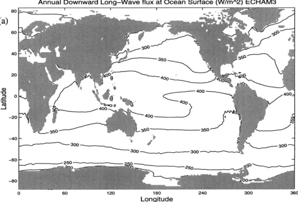
Figure 3.8 Annual mean downward longwave radiation flux at ocean
surface for ECHAM3 and ECHAM4 T106 ... 75
Figure 3.9 Annual mean zonal mean downward longwave radiation flux
at ocean surface for ECHAM3 and ECHAM4 T106 ... 76
Figure 3.10 Difference of downward long-wave radiation flux at ocean surface between ECHAM3 and ECHAM4 T106, for annual
m ean and zonal m ean ... 77
OWMNIMMMUMMOMMU11-Figure 3.11 Figure 3.12 Figure 3.13 Figure 3.14 Figure 3.15 Figure 3.16 Figure Figure 3.17 3.18 Figure 3.19 Figure 3.20 Figure 3.21 Figure 3.22 Figure 3.23 Figure 3.24 Figure 3.25
Annual mean global planetary albedo for ECHAM3 and
EC H A M 4 T 106 ... 78
Annual mean zonal mean planetary albedo for ECHAM3 and
ECH A M 4 T 106 ... 79
Difference of global planetary albedo between ECHAM3 and
ECHAM4 T106, for annual mean and zonal mean ... 80
Annual mean total cloud cover over ocean for ECHAM3 and
EC H A M 4 T 106 ... 81
Annual mean zonal mean total cloud cover over ocean for
ECHAM 3 and ECHAM4 T106 ... 82
Difference of total cloud cover over ocean between ECHAM3
and ECHAM4 T106, for annual mean and zonal mean ... 83
ISCCP-C2 8 year mean total cloud amount observation ... 84
Annual mean latent heat flux at ocean surface for ECHAM3
and ECH A M 4 T 106 ... 85
Annual mean zonal mean latent heat flux at ocean surface for
ECHAM 3 nd ECHAM4 T106 ... 86
Difference of latent heat flux at ocean surface between ECHAM3
and ECHAM4 T106, for annual mean and zonal mean ... 87
Annual net heat flux at ocean surface for ECHAM3 and ECHAM4
T 106 m odel ... 88
Annual mean zonal mean net heat flux at ocean surface for
ECHAM 3 and ECHAM4 T106 ... 89
Difference of net heat flux at ocean surface between ECHAM3
and ECHAM4 T106, for annual mean and zonal mean ... 90
Annual mean zonal mean meridional total oceanic heat transport
for ECHAM3 and ECHAM4 T106 ... 33
Figure 3.26 Annual mean zonal mean meridional heat transport in Atlantic Ocean and in Indo-Pacific Ocean for ECHAM3
and ECH A M 4 T 106 ... 35 Figure 3.27 The difference of implied total oceanic heat transport between
ECHAM 3 and ECHAM4 T106 ... 37
Figure 3.28 Annual mean total northward atmospheric meridional heat
transport simulated by ECHAM3 and ECHAM4 T106 ... 37
Figure 3.29 The "hybrid" total oceanic heat transport for ECHAM3 and
ECHAM 4 T106 m odels ... 39
Figure 3.30 25 year mean net radiation flux at ocean surface for ECHAM4
Gisst T42 model, both annual mean and zonal mean ... 91
Figure 3.31 25 year mean absorbed shortwave radiation flux at ocean surface for ECHAM4 Gisst T42, for both annual mean and
zonal m ean ... 92
Figure 3.32 25 year mean downward longwave radiation flux at ocean surface for ECHAM4 Gisst T42, for both annual mean and
zonal m ean ... 93
Figure 3.33 25 year mean planetary albedo for ECHAM4 Gisst T42, for
both annual mean and zonal mean ... 94
Figure 3.34 25 year mean total cloud cover for ECHAM4 Gisst T42, for
both annual mean and zonal mean ... 95
Figure 3.35 25 year mean latent heat flux at ocean surface for ECHAM4
Gisst T42, for both annual mean and zonal mean ... 96
Figure 3.36 25 year mean net heat flux at ocean surface for ECHAM4 Gisst
T42, for both annual mean and zonal mean ... 97
Figure 3.37 Comparison of simulation of the global mean shortwave radiation flux absorbed at the surface (in (a)), and the downward longwave radiation flux at surface (in (b)) among
AGCM s. Referring to Figure 2.1 ... 98
Figure 3.38 Annual mean meridional northward total oceanic heat transport
Figure 3.39
Figure 3.40
Figure 3.41
Figure 3.42
25 year mean northward total atmospheric heat transport
for ECH A M 4 G isst T42 ...
Annual mean total heat transport at the top of the atmosphere for ECHAM4 Gisst T42, T106 and ERBE observation ...
Annual mean "Hybrid" oceanic heat transport for ECHAM4 Gisst T42 calculated from EABE observation ...
25 year mean meridional northward oceanic heat transport for
ocean basins, ECHAM 4 Gisst T42 ...
Figure 4.1 Annual mean precipitable water vapor for ECHAM3 T106 ...
Figure 4.2 Annual mean precipitable water vapor for ECHAM4 T106 ...
Figure 4.3 Annual mean zonal mean precipitable water for both ECHAM3 and EC H A M 4 T 106 ...
Figure 4.4 NVAP analysis of annual mean precipitable water, and zonal mean ....
Figure 4.5 Annual mean total precipitation for ECHAM3 T106 ...
Figure 4.6 Annual mean total precipitation for ECHAM4 T106 ...
Figure 4.7 Annual mean zonal mean total precipitation for both ECHAM3 and EC H A M 4 T 106 ...
Figure 4.8 Annual mean total precipitation by Global Precipitation Climatology Project (G PC P ) ...
Figure 4.9 Annual mean evaporation for ECHAM3 T106 ...
Figure 4.10 Annual mean evaporation for ECHA T106 ...
Figure 4.11 Annual mean global moisture flux for ECHAM3 T106 ...
Figure 4.12 Annual mean global moisture flux for ECHAM4 T106 ...
Figure 4.13 Annual mean zonal mean moisture flux for ECHAM3 T106 and ECH A M 4 T 106 ... 99 100 100 101 106 106 107 107 108 108 109 109 110 110 111 111 112
Figure 4.14 Annual mean moisture transport for ECHAM3 T106,
ECHAM4 T106 and for Baumgartner & Reichel ... 112
Figure A. 1 Difference of total heat transport in Atlantic Ocean and
Indo-Pacific Ocean for ECHAM3 and ECHAM4 T106 ... 113
Figure A.2 Heat transport carried by ocean surface net shortwave radiation in
ECHAM3 and ECHAM4 T106 Atlantic, with their difference ... 114
Figure A.3 Heat transport carried by ocean surface net shortwave radiation in
ECHAM3 and ECHAM4 T106 Indo-Pacific, with their difference ... 115
Figure A.4 Heat transport carried by ocean surface downward longwave radiation in ECHAM3 and ECHAM4 T106 Atlantic,
w ith their difference ... 116
Figure A.5 Heat transport carried by ocean surface downward longwave radiation in ECHAM3 and ECHAM4 T106 Indo-Pacific,
w ith their difference ... 117
Figure A.6 Heat transport carried by ocean surface net latent heat flux in
ECHAM3 and ECHAM4 T106 Atlantic, with their difference ... 118
Figure A.7 Heat transport carried by ocean surface laten heat flux in ECHAM3 and ECHAM4 T106 Indo-Pacific, with their difference ... 119
Acknowledgment
I would like to thank my advisor, Dr. Peter Stone, for suggesting this study, for all the time
Chapter 1
Introduction
1.1 Background
General Circulation Climate Models (GCMs) are believed to have the potential to simulate the global scale dynamic and thermodynamic processes, and to calculate explicitly the large-scale interactions such as exchanges of mass, momentum and energy across the interfaces of the earth's climate subsystem. In view of the GCM's high capacity to simu-late the climate under a great variety of boundary conditions, the model constitutes a pow-erful tool for climate research studies. Many of the major operational weather centers around the world have been developing and using their GCMs in an attempt to explain the causes of climate variability, to obtain a better understanding of the observed climate
changes, and to predict the possible climate state in the future.
The core of all numerical models is a set of equations expressing the general physical prin-ciples of conservation of mass, momentum and energy, and the chemical laws that govern the composition of the components of the climate system. These three-dimensional equa-tions are nonlinear and each variable in the equaequa-tions is interrelated to the others. Any change in one of these variables may induce variations in others and in turn generate a feedback in the original variable. Normally, in passing from these governing equations to the working climate model several steps are followed: (1) the discretization and choice of
resolution, (2) the parametrization of physics, (3) the integration in time, (4) the verifica-tion, (5) the model improvement. Each of these steps has its characteristic difficulties and thus may introduce errors and uncertainties that compromise the model simulated climate to a greater or lesser extent.
While the numerical methods and resolutions used in the GCMs to solve the equations are relatively standard and well known, the same cannot be said for the parameterizations of a wide range of physical processes which occur on scales too small to be resolved by the models. These physical processes are referred to as subgrid-scale processes including, for instance, the occurrence of convection, cloudiness and precipitation. The subgrid-scale processes must be parameterized in terms of variables which are resolved by GCMs, and in principle it is this parameterization which makes GCMs different from each other. It may also account for some of the models' successes as well as some of their failures. For example, the study of GCMs' performance and limitations by Stone and Risbey (1990) "point[ed] out that the meridional transports of heat simulated by GCMs used in climate change experiments differ[ed] from observational analysis and from other GCMs by as much as a factor of two." In addition, they "demonstrate that GCM simulations of the large scale transports of heat are sensitive to the (uncertain) subgrid scale parameterizations."
Besides, the earth's climate system is composed of the atmosphere, hydrosphere, cryo-sphere, land surface and biosphere and their interactions. These subsystems have very dif-ferent response time scales and their interactions are not fully understood, but are known to be complex and to produce feedbacks. So, the solutions of the climate governing equa-tions involve a great deal of computation, starting from some initialized state and investi-gating the effects of changes in a particular component of the climate system. Boundary conditions, for example the solar radiation, SSTs or vegetation distribution, are set from observational data or other simulations. These data are rarely complete or of adequate accuracy to specify completely the environmental conditions, so that there is inherent uncertainty in the simulation results. On the other hand, all the uncertainties inherent in
GCMs leave room for model improvement.
With the complexity and difficulties in simulating the climate system mentioned above, among many other reasons, together with the consideration of available computer resources, historically many GCM communities start with a component GCM such as Atmospheric GCM (AGCM) and Ocean GCM (OGCM) which may be coupled with other components in the future to simulate the whole climate system.
The ability of current atmospheric models to simulate the observed climate varies with scale and variable. Given the correct sea surface temperature (SST), most models simulate the observed large-scale climate with skill, and give a useful indication of some of the observed regional interannual climate variations or trends, as well as the characteristic inabilities of a particular model. The simulation of clouds and their radiative effects remains a major area of difficulty, and AGCMs generally are not expected to simulate the local climate with fair accuracy (Risbey and Stone, 1996). The evaluation of the climate simulation capability of component Ocean GCMs (OGCMs) shows that they realistically portray the large-scale structure of the ocean gyres and the gross features of the thermoha-line circulation. OGCM's major deficiencies are the representation of mixing processes, the structure and strength of western boundary currents, the simulation of the meridional heat transport, and the portrayal of convection and subduction.
AGCMs are developed by using specified lower boundary conditions (SSTs, sea-ice extent, etc.), and OGCMs are integrated with specified surface wind stresses, and/or relax-ation of surface temperature and salinity to climatological values. These models' behav-iors are strongly constrained by the prescribed boundary conditions. Upon coupling, with the removal of the constraint of boundary conditions, the coupled GCMs are known to have a dramatic climate drift of its ocean-atmospheric system. Currently, most coupled models use "flux adjustment" whereby the heat and fresh water fluxes (and possibly the surface stresses) are modified before being imposed on the ocean by the addition of a
"cor-rection" or "adjustment.
It is expected that this conflict between the use of a fully physically based model and the use of a non-physical flux adjustment will be reduced as models are further improved. Some modelers even draw an encouraging analogy with the early development of numeri-cal weather prediction when ad hoc corrections were used to improve forecasts. Later improvements in model formulation and initialization techniques made such corrections unnecessary.
The purpose of model improvement and ultimately the understanding and predictive abil-ity of climate may be achieved by the systematic model intercomparison and evaluation which can provide valuable information for model improvement with the in-depth diagno-sis and interpretation of model results. (e.g., Atmospheric Model Intercomparison Project; Gates, 1992).
1.2 Motivation
According to "Climate Change 1995, The Science of Climate Change" (IPCC, 1995), "the major areas of uncertainty in climate models concern clouds and their radiative effects, the hydrological balance over land surfaces and the heat flux at the ocean surface", and "the comprehensive diagnosis and evaluation of both component and coupled models are essential parts of model development, although the lack of observations and data sets is a limiting factor."
The heat flux at the ocean surface can be used to calculate the mean state of the implied meridional northward oceanic heat transport with the assumption that there is no heat transport across the sea shore. The discrepancy in the simulation of the ocean surface heat
flux among the AGCMs would be exaggerated in the calculation of the oceanic heat trans-port. Further, the estimate of implied oceanic heat transport is also an important index of an AGCM's simulation abilities.
Studies indicate that there are great discrepancies in the estimate of annual mean total oce-anic heat transport by using various GCM models (this occurs even in the observational estimates). Few studies have further investigated the roles taken by the three major ocean basins: Atlantic Ocean, Pacific Ocean and Indian Ocean in contributing to the discrepancy. We will carry out the calculation for the Atlantic Ocean and Indo-Pacific Ocean based on a conceptual division of the total ocean, and seek a clearer picture of how the two major ocean basins contribute to the total oceanic heat transport.
The surface energy budget is tightly related to the surface water budget, which is another major area of uncertainty in climate models especially over land surfaces; thus we are also motivated to carry out diagnostic studies of both ECHAM models's hydrological balance and compare with available data such as surface moisture flux, precipitation and evapora-tion, etc.
Since the dataset we use is from two model runs, that is, the 10 year means for ECHAM3
T106 and ECHAM4 T106, the intercomparison between these two models and the
com-parison with other models and available observations will provide the useful information for model improvement. Thus, it will give us a clue of model behavior requiring modifica-tion, and portray possible reasons for model failure.
Another calculation we carry out in this study is how much of the oceanic heat transport is explained (or carried) by the surface heat flux components. We would like to investigate, for example, how much heat would be transferred meridionally by the latent heat flux component alone. We should expect these flux components to act differently in the total oceanic heat transport, and in the ocean basins' heat transport as well.
1.3 Thesis Structure
This section provides a brief overview of the thesis structure and organization. The thesis itself is divided into six chapters:
- Chapter 1 introduces the background of the thesis work, the motivation of the study, along with this thesis structure introduction.
- Chapter 2 describes the model history, structure and the improvements implemented in the two generations of models studied in the thesis. The description of datasets is included.
- The calculation for the model implied oceanic heat transport will be presented in Chapter 3. There are five major sections - the methodology, the correction schemes, the annual mean of ocean surface heat fluxes, the model implied meridional oceanic heat transport (for ocean total, and ocean basins), the oceanic heat transport with other boundary conditions and horizontal resolution, and the oceanic heat transport carried
by the different heat flux components.
- The model's simulation of surface hydrological balance and related diagnosis would form Chapter 4. There are six sections in the chapter.
- Chapter 5 will summarize the studies performed. Important conclusions will be drawn.
- Chapter 6 is the major reference section.
- Appendix includes the calculation of the meridional northward oceanic heat transport carried by the different heat flux components, and the discussion on their roles in transferring the heat for the energy balance of the climate system.
Chapter 2
Model Description and Data Sets
2.1 Model History and Description
The ECHAM atmospheric general circulation models are a series of models developed at MPI. The earliest version, ECHAMO, evolved from the cycle 17 version (operational in 1985) of the numerical weather prediction model at the European Center for Medium-Range Weather Forecasts (ECMWF). Since ECHAMO, the models developed at MPI are the second generation ECHAMI and ECHAM2, the third generation ECHAM3 and the fourth ECHAM4. The models we are using in this diagnostic study are ECHAM3 and ECHAM4 T106 AGCMs. They have a horizontal spectral resolution with a 320 (longi-tude) x 160 (latitudes) Gaussian transform grid mesh and 19 vertical levels. The vertical coordinate used in ECHAM3 and ECHAM4 is a hybrid -p-coordinate system, with smooth transition from G-coordinates at the surface to p-coordinates at the top of the atmosphere.
The standard configuration of ECHAM3 and ECHAM4 GCMs are ECHAM3 T42 and ECHAM4 T42 respectively, whose horizontal resolution corresponds to a 128 (longitude) x 64(latitude) Gaussian transform grid. T106 are their test versions. The model formula-tion and parameterizaformula-tions are identical for T42 and T106 versions for both ECHAM3 and ECHAM4 except for two things: 1) the horizontal diffusion coefficients were made
resolu-tion dependent such that the slope of the spectral kinetic energy comes closer to observa-tions; 2) a rain efficiency parameter in the cloud scheme was made resolution dependent, which influences the cloud lifetime and thereby the associated planetary albedo, in order to match the global annual mean top of atmosphere radiative fluxes with the Earth Radia-tion Budget Experiment (ERBE) satellite observaRadia-tions.
The formal documents for ECHAM3 T42 and ECHAM4 T42 have been published by MPI. In table 1, we outline the model configurations. More details can be found in the Max-Planck-Instutut fir Meteorologie Report No. 93 (Roeckner et al 1992) and Report No. 218 (Roeckner et al 1996).
As the immediate preceder of ECHAM4, ECHAM3 T42 has been tested in many studies (e.g. Gleckler et al, 1995; Gaffen et al., 1996). It is also the AMIP (Atmospheric Model Intercomparison Project) (Gates, 1992) MPI baseline model. The model has generally per-formed outstandingly in the studies (Lau et al. 1996).
Most of the structure and parameterizations of ECHAM3 T42 have been carried forward to ECHAM4 T42, while they differ most sharply in the treatment of transport and diffu-sion, of chemistry and radiation, and of the planetary boundary layer (PBL). The parame-terization of convection, cloud formation and surface characteristics have also been modified. The author would like to highlight here the three improvements made in ECHAM4: 1) The advection of water vapor, cloud water and chemical species are calcu-lated by the shape-preserving semi-Lagrangian transport scheme rather than a spectral transform method; 2) the shortwave radiation is treated by the two-stream method of Fon-quart and Bonnell (1980), the long-wave radiation by the method of Morcrette (1991); and
3) the calculations of shortwave absorption by atmospheric water vapor and longwave
absorption by the 7-12 micron water vapor continuum are improved (Giorgetta and Wild,
1995). Figure 2.1 shows the result of one test integration completed at ETH, which
This improved treatment is significant for the calculations of model implied oceanic meridional heat transport.
Table 1. Information for ECHAM3 T42 and ECHAM4 T42 GCMs.
ECHAM3 T42 L19 ECHAM4 T42 L19 Dynamics/Numerics * Spectral (Baede, et al, 1979), but The same as in ECHAM3, except that
* With revised formulation of the pres- * The horizontal advection of water sure gradient term (Simmons and vapor and cloud water are treated by
Chen, 1991) shape-preserving semi-Lagrangian
transport (SLT) scheme (William-son and Rasch, 1994)
* The vertical advection of positive definite quantities is treated by SLT scheme
Horizontal diffusion * Enhanced scale selectivity (Laursen * linear tenth-order horizontal
diffu-and Eliasen, 1989), sion is applied to all prognostic
vari-* The diffusion coefficients were cho- ables below about 150hpn,
sen such that the slope of the spec- * in the model stratosphere, the order
tral kinetic energy is close to of the scheme is reduced
incremen-observations. tally to second-order at the upper
two model levels
Chemistry * AMIP C02 concentration * Trace constituents including
meth-ane, nitrous oxide, and 16 different CFCs are added
Radiation * Hense et al., 1982; and Rockel et al., * Shortwave radiation is treated by the 1991. two-stream method of Fonquart and
Bonnell (1980),
* Longwave radiation by the method of
Morcrette (1991).
* In addition, further changes are made
in the treatment of other gaseous absorbers, continuum absorption by water vapor, and cloud-radiative interactions.
Vertical diffusion * Louis (1979), but * A higher-order closure scheme after * with low wind correction according Brinkop and Roeckner (1995) to to Miller et al. (1992). compute the vertical diffusion of * The Richardson number is revised to momentum, heat, moisture, and
Surface absorbed SW Surface LW down 180 160 I-140 F 120 F 340 F 320 F 300 F 100' U 91X = 0 K~ > X
Figure 2.1 Comparison of simulations of the surface heat balance by ECHAM GCMs together with various atmospheric GCMs. On the left is the global mean annual mean shortwave radiation absorbed at the surface, and on the right the global mean annual mean longwave radiation incident on the surface. Observational values are based on the Global Energy Balance Archive (Ohmura and Gilgen, 1993; Wild et al 1995).
ECHAM3 T42 L19 ECHAM4 T42 L19 Convection * Tiedtke (1989) for deep midleval and The same as in ECHAM3
shallow convection, * With modifications after Nordeng
* Stratocumulus convection according (1996)
to Tiedtke et al. (1988) * The closure assumption is also modi-fied: cloud-base mass flux is linked to convective instability instead of moisture convergence.
Soil processes * Five layer model for heat transfer, The same as in ECHAM3, except that
* Refined bucket model for soil mois- The heat capacity, thermal
conductiv-ture; ity, and field capacity for soil
mois-* Vegetation effects included (Blondin, ture are prescribed according to
1989) geographically varying values
* Sea ice temperature is calculated derived from Ford and Agriculture from the net heat fluxes including Organization (FAQ) type distribu-conductive heat transfer through ice tions (Patterson, 1990, and Zobler,
1986). 185 182 171 173 175 162 164 147 142 350 342 337 335 334 326 315 311
2.2 Data Set
The data set used in this research is a part of the ten-year-mean output of the official
ECHAM3 and ECHAM4 T106 L19 model runs provided by Mr. Wild Martin at Swiss
Federal Institute of Technology, Zurich, Switzerland. This data set is mainly confined to the model's simulation of surface energy budget and water budget. The main fields included are:
* Annual mean global distribution of surface latent heat flux. - Annual mean global distribution of surface sensible heat flux
- Annual mean global distribution of surface short-wave radiation, including the upward and downward partition.
- Annual mean global distribution of surface long-wave radiation, including its upward and downward partition.
- Annual mean - Annual mean - Annual mean - Annual mean - Annual mean - Annual mean global global global global global global
distribution of total cloud cover. distribution of surface albedo.
distribution of vertically integrated precipitable water vapor. distribution of evaporation.
distribution of precipitation. distribution of river runoff
Chapter 3
Oceanic Heat Transport Calculation
In this chapter, we will first introduce the methodology and correction schemes we used, and present the simulated mean state of the total heat flux and the component fluxes at the ocean surface. The model implied meridional northward oceanic heat transport for the whole ocean and ocean basins will be calculated and compared with some other calcula-tions and available observational study.
3.1 Methodology
The estimation of global mean annual mean oceanic meridional heat transport can be obtained by several methods. Generally, the methods can be separated into three major categories: residual method, direct estimate and surface heat-balance method. All these methods have their associated advantages and disadvantages. The method used in this research is the so-called "classical method", i.e., the surface heat-balance method, which calculates the meridional northward oceanic heat transport from the heat balances at the ocean surface.
A schematic of the atmosphere-ocean system is shown in Figure 3.1, with Fs as the net sea
surface, downward heat flux, which includes the net sea surface radiative flux Rs, net sea surface latent heat flux LH and net sea surface sensible heat flux SH; and F0, FA as the
ver-tically integrated divergent heat fluxes in the Ocean and in the atmosphere respectively; R is the net radiation flux at the top of the atmosphere. The bracket in Figure 3.1 means the zonal average. All quantities are the annual mean.
[R]
Top of atmosphere
South North
Figure 3.1 Schematic of heat fluxes in the atmosphere-ocean system. North-ward heat fluxes are defined as positive, as are downNorth-ward vertical fluxes. The brackets are for the zonal mean.
The energy equation for the oceans can be written as:
S0+VH* F0 = Rs+ LH + SH
where:
(1)
S, heat storage in the oceans
VH- horizontal divergence
In the annual mean, S, vanishes as long as no long-term temperature change is observed. The equation then becomes:
Atmosphere
[A] [F [A]
-*4 Ocean
(2)
VH F F = R-VHeFA = F = RS+LH+SH
If we take the zonal average of equation (2), we have
- -a
[F ]
a cos~paqp
coswp = [Fs] Since the northward oceanic heat transport at latitude (p is:T,(p) = 21cacosp[Fj(p)]
where a is the earth's radius, we have 1 2
2xta cosqp
a [T(p)] = [Fs] a ( = 2ta 2costp[Fs](6)
Integrating equation (6) starting from the north pole, the implied meridional oceanic heat transport across a latitude circle (po is:
IC
p= -2 2
a
2[Fs]cos(pd(pT 0(
9 0 = -
9
0 (7)Equation (7) is the basic equation we will use to calculate the model implied oceanic meridional heat transport. This method implicitly assumes that there is no heat flux across the land-sea boundary.
(3)
(4)
i.e.,
3.2 Correction Scheme
Because of the existence of an imbalance in global mean surface heat flux over oceans, the integration of equation (7) at the south pole will not result in zone transport, as it should be. We need to apply the correction method to correct it.
As discussed in Carissimo et al., 1985, there are many correction methods based on differ-ent considerations. We will adopt here the same symbols as in Carissimo's work, where a subscript NP indicates the integration was carried out starting at the north pole, and a sub-script SP represents a calculation starting from the south pole. A supersub-script * means the transport is uncorrected.
(1) Standard method, which applies a constant correction to all the original values.
P
T
T0(y) - TONP
2 2cosgdp
= T *() - - T -- l(1 - sing) (8)
ONP 2 ONP 2
The calculation is uniformly applied to unit area at each latitudinal circle. So there is no bias between the high latitudes and low latitudes. We will apply this correction scheme to all the heat transport calculations in this thesis.
(2) the correction varies with latitude as in Saunders et at., 1983, which mainly affects the low latitudes based on the consideration of reflected radiation associated with the diurnal
cycle of the albedo:
ONP ONP*(
This scheme affects the tropical regions mostly since the over that region.
(3) the correction weighted average of TONP* and Tos,*
T9()) =TONP OSP
e
sin
2e9
(9)
mean surface albedo is highest
(10)
The effect of this correction schema depends on the distribution of the uncorrected heat transport. In our case, the correction of flux is larger in the midlatitudes than in the tropics.
In this thesis, we use the standard method to correct the non-zero oceanic heat transport at the south pole induced by the imbalance of heat flux at ocean surface.
3.3 Heat Fluxes at Ocean Surface
The surface heat fluxes across the surface, which is the boundary between the atmosphere and ocean or the land, is an essential part of the climate system as are the fluxes at the top of the atmosphere. The geographic distribution of the surface heat fluxes determines the
To(p)
= TONP*(p
)
J
22 2cos (pd
distribution of surface temperature, the amount of energy flux available to evaporate the surface water and hence the intensity of the hydrological cycle. The understanding of the heat balance at the surface is a necessary part of understanding climate and its dependence on external constraints. Therefore, it is important for GCMs to simulate the surface heat fluxes accurately when attempting to simulate the past, current and future climate.
The surface heat fluxes include the net radiative heat flux from the overlying atmosphere into the surface, the latent heat flux and the sensible heat flux at the surface, as expressed in the following equation:
Fsfc = FSfc net + SHsfc + LHsfC
-rad net net (1
where the superscripts sfc means surface, subscript rad means radiative, SH is sensible heat flux, LH the latent heat flux.
Since the net input flux of radiative energy to the surface is the sum of the net shortwave and longwave heat fluxes, we re-write (11) as:
FSfc = F fc -Ffc +F Fc Sfc1"
rad sw sw 1w (12)
where T means upward, I means downward; subscript sw means the shortwave, 1w means the longwave. Here we define the downward heat flux as positive.
Several key physical properties of the ocean let it play the critical role in the climate sys-tem: it has a low albedo when unfrozen; it has a large heat capacity; it is fluid and it covers most of the earth's surface area. Even overlain by the atmosphere, the ocean receives more than half of the energy entering the climate system. It also gives much of the ocean absorbed shortwave radiation to the atmosphere through evaporation, making the ocean the primary source of water vapor and heat for the atmosphere.
To analyze the meridional northward oceanic heat transport calculated from the surface heat-balance, we present here the model simulated annual mean heat fluxes at the ocean surface in Figures 3.2 to 3.23, among which are figures for the annual mean, zonal mean and the corresponding difference between ECHAM3 and ECHAM4, together with some related fields. All these figures are positioned after Chapter 6.
Both ECHAM3 and ECHAM4 T106 AGCMs show that, in Figure 3.2 and Figure 3.3, the net radiation flux is greatest over the tropical oceans. In that region the net radiation flux exceeds 150 w/m2, and in ECHAM3 in central tropical Pacific Ocean, it exceeds 200w/m2. Along 60 N, there are minima showing in the global annual mean distribution and their corresponding zonal means, which are associated with the annual mean location of Inter-Tropical Convergence Zone (ITCZ).
The variation of the net radiation flux with latitude and surface conditions is systematic. The low latitudes have the higher radiation surplus, and the high latitudes have the lower one. In southern hemisphere, the radiation flux contours(eg., 100 w/m2 and 50 w/m2) are
aligned along latitude circles, while in the northern hemisphere the contours are tilted due to surface effects.
The net radiation variation with the latitude can also be clearly seen in the zonal mean fig-ures. Because of the tilting in the northern hemisphere, the change of zonal mean net radi-ation flux with latitude is slower in the northern hemisphere.
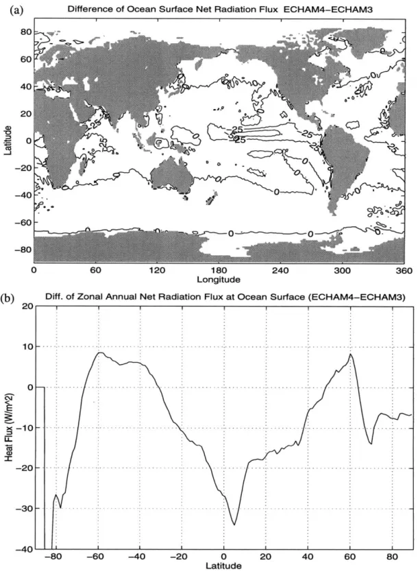
The difference of the net radiation flux at the ocean surface for annual mean and zonal mean between ECHAM3 and ECHAM4 indicates the effect of the modification of the radiation scheme from ECHAM3 to ECHAM4. In Figure 3.4(a) and Figure 3.4(b), the most significant pattern is in the tropical Pacific Ocean. ECHAM4 has much less (more than 50 w/m2) net radiation flux input into the ocean than does ECHAM3 along 60N in
dif-ference is more than 30 w/m2 at 60N. On the other hand, in the zonal mean difference, the
ECHAM4 ocean has a larger net radiation flux surplus in the southern hemisphere mid-and high latitudes mid-and northern hemisphere high latitudes. The required heat transport by the ocean poleward from the tropics must be smaller in ECHAM4.
If we break down the net radiation flux into its shortwave and longwave components and
up- and downward directions, as shown in figures from Figure 3.5 to Figure 3.10, we can see that the peak difference at 60 N with a value of -34 w/m2 results from -46 w/m2 of zonal mean absorbed shortwave radiation component flux, and 17 w/m2 of zonal mean downward longwave radiation flux component. To draw a conclusion on whether the air in the ECHAM4 model absorbs more incoming shortwave radiation, we need to look at the Top of the Atmosphere.
Figure 3.11 to Figure 3.13 present the ECHAM models' mean state (annual mean and zonal mean, together with their difference) for planetary albedo. There is almost 1% change of the global mean value, with 32.43% in ECHAM4 and 33.35% in ECHAM3.
Although the global mean value decreases in ECHAM4, the difference of the quantity for annual mean and zonal mean shows that the decrease occurs mainly in high latitudes while there is an increase in low latitudes in ECHAM4. The largest increase is over tropical Pacific Ocean along 60N; the tropical Atlantic Ocean has a minor contribution.
Since both ECHAM3 and ECHAM4 models use the same solar constant, the difference in the mean planetary albedo between the two models reflects the difference in the mean out-going shortwave radiation at the top of the atmosphere. Therefore, over the tropical oceans at the top of the atmosphere there would be less net incoming shortwave radiation while there would be more net incoming shortwave radiation over other regions in ECHAM4. Together with the Figures 3.5 to 3.10, we may infer that, due to the radiation scheme mod-ification in the ECHAM4 T106 AGCM, the atmosphere over the oceans absorbs or reflects much more incoming shortwave radiation in ECHAM4 than in ECHAM3. Consequently,
the underlying ocean in ECHAM4 receives less incoming shortwave radiation but more downward longwave radiation from a cloudier atmosphere. The compensation makes the changes in the net radiation flux less than in the absorbed shortwave radiation. From the global mean point of view, ECHAM4 has a more realistic (i.e., closer to the observations,
see in Figure 2.1) radiation scheme.
The mean state of model simulated total cloud cover in Figure 3.14 to Figure 3.15, together with their corresponding difference in Figure 3.16, also shows the effect of modi-fication to the radiation scheme. We also include in Figure 3.17 the ISCCP-C2 8-year mean total cloud amount observation which is the International Satellite Cloud Climatol-ogy Project (established in 1982 as part of the World Climate Research Programme (WCRP)) Stage 2 analysis for the months July 1983 through June 1991. Compared against the ISCCP data, ECHAM4 has simulated fairly accurately the total cloud cover distribu-tion for the northern Atlantic Ocean, where the ECHAM3 apparently has too low total cloud cover. The similar too low total cloud amount pattern can be found in ECHAM3 southern Atlantic Ocean. For the Pacific Ocean, the large area of low cloud amount in the tropical Pacific Ocean is not shown in ECHAM4 but ECHAM3 has a good representation for this region. But the overall pattern matching in the Indo-Pacific Ocean is much better in ECHAM4 than in ECHAM3. The global mean total cloud cover is -50% in ECHAM3 and -59% in ECHAM4. The ECHAM3's total cloud cover is too low.
If comparing Figure 3.10(a) with Figure 3.16(a), the total cloud cover increase in the
east-ern Pacific and Atlantic Oceans in ECHAM4 corresponds to the increase of downward longwave radiation over those regions.
The evaporative heat loss from the ocean surface (LH flux in Figure 3.18 to Figure 3.20) in both models has the greatest values over the midlatitudes and the warm western boundary currents. In the western region of the Pacific and Atlantic oceans, the latent heat loss may exceed 200 w/m2 which is much greater than the local net radiation heating to the ocean
surface. The latent heating cooling of the ocean surface is also large over the subtropical oceans, which offsets most of the heating to the ocean surface by the net radiation.
Along the equator, there is a "tip" in the zonal mean latent heat flux (Figure 3.19) in both models, showing a greater reduction (-40 w/m2) of evaporation heat lose to the atmo-sphere. It results from lower evaporation over the relatively cold ocean water flowing from the eastern ocean to the western ocean region (northern and southern equatorial currents).
The pattern of the difference of zonal mean latent heat flux at ocean surface between
ECHAM3 and ECHAM4 is very different from those of the radiation fluxes. It goes up
and down more frequently, and is mostly positive (more evaporative heat loss in ECHAM4). The value is greater in the Northern Hemisphere, indicating a larger modifica-tion effect there, though it is hard to say the modificamodifica-tion is really an improvement.
The sensible heat loss (figures not included in this thesis) from the ocean surface is small in both models, except over the warm western boundary currents of the midlatitude oceans. Over that region, when cold air from the continents flows over the warm ocean surface (mainly during winter), a large sensible heat flux occurs. It may exceed 50 w/m2 in the annual mean. But it is still much less important to the mean surface net heat flux than
is the latent heat flux. (The difference between the two models is small too!)
Adding the net radiation flux, the latent heat flux and sensible heat flux together, we obtain the net heat flux at the ocean surface, as shown in Figure 3.21 to Figure 3.23. In both
ECHAM3 and ECHAM4 AGCMs, the net heat flux is large and negative over the western
boundary currents, where the ocean is supplying the energy through heat transport by the ocean currents and then heating the atmosphere. In the equator and the eastern regions of the ocean, the atmosphere is heating the oceans (with positive net heat flux at the ocean surface) where upwelling brings the cold water from the deep ocean to the ocean surface. We have seen that in these regions the evaporative cooling in reduced and the net radiation
is used to heat the ocean. Ultimately, the energy will be transferred to mid- and high lati-tudes and then lost back to the atmosphere. This heat transport from the tropical and east-ern oceans to mid- and high latitudes plays a critical role in determining the energy cycle of the climate system.
The difference of the net heat flux between the two ECHAM models (Figure 3.23) has negative values within ±300 latitude, and positive values over other regions. Since the net heat flux is positive in low latitudes and negative in mid- and high latitudes, the difference indicates that, in tropical regions the ECHAM4 model's ocean receives less net heat flux than does the ECHAM3's ocean; on the other hand, in mid- and high latitudes the ECHAM4 ocean loses less net heat to the atmosphere than the ECHAM3 ocean. We also notice the relatively large area of positive net heat flux around 500 S in ECHAM4, which may induce an equatorward heat transport.
3.4 Meridional Northward Oceanic Heat Transport
The radiative energy budget of earth's climate system is characterized by strong input of solar energy at low latitudes and a back radiation to space which is more uniformly distrib-uted over the globe. On an annual mean basis, the net radiative energy budget of the cli-mate system must be balanced, which implies the existence of a net poleward heat transport by the atmosphere and oceans combined in both hemispheres. This combined atmospheric and oceanic meridional heat transport can be estimated with high accuracy from satellite radiation measurements of the net radiation budget at the top of the atmo-sphere. It is interesting to note that the apportionment of the meridional heat transport between ocean and atmosphere has been a matter of some controversy in history: meteo-rologists have tended to ascribe a greater role in meridional heat transport to the ocean than oceanographers (Bryden, 1993). Normally, meteorologists base their estimates of the oceanic heat transport on residuals of the satellite derived radiation budget and the AGCM output calculated atmospheric heat transport. The value is nearly 4 PW (lPW=1015 watts)
in mid-latitudes. On the other hand, integrations of surface oceanic heat flux over ocean derived from bulk formulas by Budyko (1974) and Talley (1984) have much lower values, typically 1 to 2 PW. These uncertainties may come from the inaccurate simulations of the surface heat fluxes by the AGCMs, lack of data over oceans, errors in the bulk formulae, and instrumental radiation measurement uncertainty at the top of the atmosphere. With the improvement of data availability and treatment of surface heat fluxes, recalculations are needed and should contribute to a better understanding of the ocean's role in transferring heat poleward and in reducing the equator-to-pole temperature gradient.
In this subsection, we will present the estimates of the global mean annual mean total oce-anic meridional heat transports as a function of latitude based on ECHAM3 and ECHAM4
T106 ten year runs. The respective estimates for the major ocean basins: Atlantic ocean,
the Pacific Ocean and the Indian Ocean have been carried out. Since the Indonesian throughflow has not been taken into account, the contributions from Pacific Ocean and Indian Ocean in this research should be combined and then represented as Indo-Pacific
Ocean.
3.4.1 Results
The mean state of the meridional northward heat transport are calculated from the annual mean net heat flux at the ocean surface using the surface heat- balance method, and cor-rected with the standard correction scheme. The results for the ocean total and ocean basins are presented in Figure 3.24 and Figure 3.26. In the discussion section, some other model simulation results and observations are included in Figures and Tables.
(1) Ocean Total
The ECHAM3 and ECHAM4 T106 implied annual mean meridional northward heat transport for ocean total are shown in Figure 3.24. In both models, the annual mean ocean transport shows a substantial asymmetry between the northern hemisphere and southern
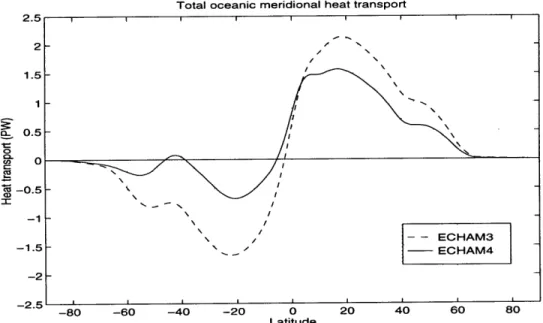
hemisphere. This asymmetry must be related to the difference in physiography of the more land-covered northern hemisphere and more ocean-covered southern hemisphere. In mid-latitudes, the heating due to the convergence of the heat transport in northern hemisphere is larger than that in southern hemisphere in both models. The highest heat transport occurs at around 200 in both models. The variation in northern hemisphere is smaller than in southern hemisphere, and we can see that, in southern hemisphere ECHAM4, even the direction of oceanic heat transport changes to equatorward.
Total oceanic meridional heat transport
2.5 -- 2- 1.5- 1- D0.5-U)0 0.5 fE A a E A TECHAM3 -1.5P at ECHAM4 -2--2.5 I -80 -60 -40 -20 0 20 40 60 80 Latitude
Figure 3.24 Annual mean zonal mean meridional total oceanic heat transport for ECHAM3 and ECHAM4 T 106.
The implied heat transport in northern hemisphere mid-latitude ocean is of the order of 2
PW. ECHAM3 and ECHAM4 show their consistency in the estimate over this region. The value is much closer to the oceanographer's estimate (1-2 PW) than that of early meteo-rologists' (-4 PW).
(2) Ocean Basins
In order to calculate the heat transport for ocean basins, we need the proper boundaries to "separate" the ocean basins from each other, and then apply the surface heat-balance method to the ocean basin's annual mean zonal mean net heat flux. The calculations for the Atlantic ocean and Indo-Pacific ocean may be questionable in the southern hemisphere beyond the Cape of Good Hope (-350S). There is a cross-basin heat transport which we totally ignore in the calculation. Generally, the calculation method used for ocean basins is only applicable to a basin which is wholly bounded by the land, or the western and eastern boundary conditions are well known.
The conceptually separated ocean basins used in this calculation are shown in Figure 3.25. We did not take into account the Indonesian throughflow, so the Pacific Ocean and Indian Ocean should be considered as one, i.e., the Indo-Pacific Ocean. Because many other stud-ies explicitly calculated the heat transport for the Pacific Ocean, we use the calculation from the Indo-Pacific Ocean to represent the value in the northern hemisphere for the Pacific Ocean since our calculation shows the heat transport in the northern hemisphere in the Indian Ocean is small.
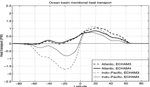
As we can see in Figure 3.26, the nature of the heat transport differs remarkably for Atlan-tic Ocean and Indo-Pacific Ocean. Northward heat transport is found at almost all latitudes in the Atlantic Ocean in both models. The difference of heat transport between ECHAM3 and ECHAM4 is small compared with that for Indo-Pacific Ocean.
The variation of total oceanic heat transport between ECHAM3 and ECHAM4 is mostly explained by their corresponding variation in the Indo-Pacific Ocean, especially in the southern hemisphere. But the asymmetry of total oceanic heat transport between southern
Schematic of Ocean Basins -20 -40 -60 -80 0 60 120 180 240 300 Longitude
Figure 3.25 The schematic of ocean basins.
Ocean basin meridional heat transport
-80 -60 -40 -20 0 20 40 60 80
Latitude
Figure 3.26 Annual mean zonal mean meridional heat transport in Atlantic Ocean and in Indo-Pacific Ocean for ECHAM3 and ECHAM4 T106.
360 -0.5 -1.5 -2 -2.5 - Atlantic, ECHAM3 Atlantic, ECHAM4 AtlndtPaic, ECHAM -.-.-.-.-.-.-.-.--.-.-.-.... - ... ... -.. Indo- P acific,.E C H A M 3 -Indo-Pacific, ECHAM4
hemisphere and northern hemisphere mainly results from the contribution of Atlantic Ocean. Generally, in the northern hemisphere, the poleward heat transport is larger in the Atlantic Ocean than that in the Indo-Pacific Ocean, while in the southern hemisphere, the heat transport by the Indo-Pacific Ocean dominates over the Atlantic Ocean.
3.4.2 Discussion
(1) Ocean Total
In the previous section we presented the characteristics of the ECHAM AGCMs' implied mean state of oceanic meridional northward heat transport. The difference in this quantity (as shown in Figure 3.27) is of great interest and important to us for the purpose of model comparison and improvement.
In Figure 3.27, at almost every latitude in both southern and northern hemisphere,
ECHAM3 has the larger poleward heat transport than has ECHAM4, except in a small
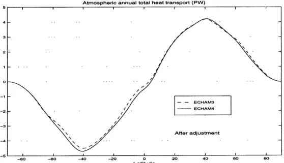
area at the equator in the northern hemisphere. In other words, Figure 3.27 suggests that the implied ocean in ECHAM4 plays a less important role in transferring heat poleward than does the ECHAM3 implied ocean. Consequently, since the total heat transport required for the balance of the earth climate system at the top of the atmosphere should be the same for both ECHAM models, the ECHAM4 model's atmosphere will transfer more heat poleward than will the ECHAM3's atmosphere. The calculation of atmospheric heat transport for the models does not support this inference, as shown in Figure 3.28.
In Figure 3.28, the atmospheric heat transport simulated in ECHAM3 and ECHAM4 are almost identical except a small difference (< 0.2 pw) spanning most areas in the southern hemisphere. Further investigation shows that the model's atmosphere seems "transparent" to the underlying ocean: the pattern of difference in oceanic heat transport between the
Difference of Total Oceanic Heat Transport 0.5-0 -0.5-ECHAM4 - ECHAM3 -80 -60 -40 -20 0 Latitude
Figure 3.27 The difference of implied total
ECHAM3 and ECHAM4 T106.
20 40 60 80
oceanic heat transport between
Atmospheric annual total heat transport (PW)
Latitude
Figure 3.28 Annual mean total northward atmospheric meridional heat transport simulated by ECHAM3 and ECHAM4 T106.
two models has been almost exactly copied to the top of the atmosphere, thus obtaining the same pattern of difference in total heat transport at the top of the atmosphere.
Gleckler et al (1995) proposed that the implied oceanic heat transport was sensitive to the radiative effects of clouds to explain the large discrepancy of this quantity among current AGCMs. They computed a "hybrid" oceanic heat transport To which includes the cloud radiative forcing with the formula:
TO=TA+O-TA~TO+ 6TCRF (13)
where:
TA+o = the atmosphere and ocean combined northward meridional heat
transport inferred from the observed 4 years net top-of-the-atmo-sphere radiation in the Earth Radiation Budget Experiment (ERBE) (Barkstrom et al, 1990).
STCRF = the difference between the observed and simulated TA+O resulting from the effects of clouds;
Their results show a remarkable improvement in the calculation of AGCMs' implied oce-anic heat transport after the cloud radiative forcing correction.
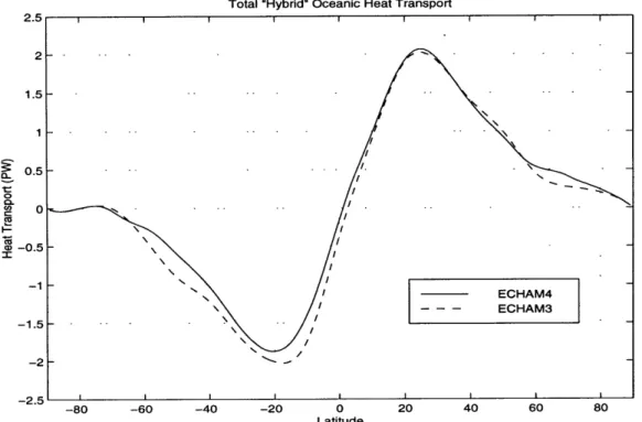
In Figure 3.29 we calculate and present the same "hybrid" oceanic heat transport as in Gleckler et al by using the same TA+o from ERBE observation. The improvement as com-pared with Figure 3.24 is also remarkable, the ECHAM3 and ECHAM4 T106 have obtained a consistent (not necessarily correct) oceanic heat transport now! To verify the reasonability of these "hybrid" oceanic heat transports, let's make the comparison against
other available observational data.
Total "Hybrid" Oceanic Heat Transport
-2.5'1
-80 -60 -40 -20 0 20 40 60 80 Latitude
Figure 3.29 The "hybrid" total oceanic heat transport for ECHAM3 and ECHAM4
T106 models.
In Table 2, we present the oceanic heat transport calculation for ECHAM3 and ECHAM4 before and after cloud radiative forcing correction, the results obtained by Macdonald and Wunsch (1996), and by Trenberth and Solomon (1994). The Macdonald and Wunsch's estimate was derived by integrating hydrographic velocity data over the rapid spatial vari-ations that they show. Trenberth and Solomon used operational weather prediction analy-sis produced by the European Centre for Medium Range Weather Forecasts (ECMWF). These two data sets are believed to be reliable.
Table 2. Comparison of total oceanic heat transport calculation (PW)
Latitude hybrid hybrid ECHAM3 ECHAM4 Macdonald Trenberth
ECHAM3 ECHAM4 500 N 1.0 0.8 0.8 0.55 0.55±0.3 0.57 24-250 N 2.0 2.1 2.0 1.42 1.6±0.3 2.0 100 N 1.0 1.1 1.8 1.5 1.5 100S -1.7 -1.3 -1.1 -0.3 -0.7 300 S -1.7 -1.6 -1.5 -0.4 -0.9±0.3 -0.8
In Table 2, the largest change occurs in ECAHM4 southern hemisphere low latitudes
(100S and 300 S here, as included in Table 2). Note please in Figure 3.24, that the oceanic
heat transport in the ECHAM4 southern hemisphere is small, and even equatorward around 400S. It suggests that the oceanic heat transport in the ECHAM4 southern hemi-sphere without cloud forcing correction is unreliable. On the other hand, when comparing the hybrid results with Macdonald's and Trenberth's, we may argue that this cloud radia-tive forcing correction which brings the consistency between ECAHM3 and ECHAM4 in estimating the oceanic heat transport is even worse in this case for the ECHAM AGCMs. The hybrid values at 100 S and 300 S in both ECHAM3 and ECHAM4 are nearly 1 PW larger than those in Macdonald and Trenberth.
In Figure 3.29, the asymmetry of oceanic heat transport between northern hemisphere and southern hemisphere disappears, and the distribution shows a nearly symmetric character-istic which is not appreciated due to the asymmetric physiography of northern and south-ern hemisphere.
So, our calculation suggests that, the cloud radiative forcing correction scheme can explain only to some extent the discrepancy in estimating the oceanic heat transport, and