Diversity in evolving systems : scaling and dynamics of genealogical trees

Diversity in Evolving Systems: Scaling and Dynamics of

Genealogical Trees

by

Erik Rauch

B.S., Computer Science and Mathematics

Yale University (1996)

S.M., Electrical Engineering and Computer Science

Massachusetts Institute of Technology (1999)

Submitted to the Department of Electrical Engineering

and Computer Science

in partial fulfillment of the requirements for the degree of

Doctor of Philosophy

at the

MASSACHUSETTS INSTITUTE OF TECHNOLOGY

V~

j,-

7

January 2004

@Erik

Rauch, 2004. All rights reserved.

The

aumor hereby gtvlh to

Mfr

penmtson

duMibute

pub*

pope and

elacwonic copes of this thesis

documentin whole or

in

port

A uthor

. .

.

...

Department of Electrical Engineering

and Computer Science

January 30, 2004

Certified by.

...

Gerald Jay Sussman

Matsushita Profgssor of Electrical Engineering

Thsig's Sup

ifrisor

Accepted by...

Arthur C. Smith

Chairman, Department Committee on Graduate Students

MASSACHUSETTS INSTIuTE OF TECHNOLOGY

Diversity in Evolving Systems: Scaling and

Dynamics of Genealogical Trees

by

Erik Rauch

Submitted to the Department of Electrical Engineering and Computer Science on January 30, 2004 in partial fulfillment of the degree of

Doctor of Philosophy

Abstract

Diversity is a fundamental property of all evolving systems. This thesis examines spa-tial and temporal patterns of diversity. The systems I will study consist of a population of individuals, each with a potentially unique state, together with a dynamics consist-ing of copyconsist-ing or reproduction of individual states with small modifications to them (innovations). I show that properties of diversity can be understood by modelling the evolving genealogical tree of the population. This formulation is general enough that it captures interesting features of a range of natural and artificial systems, though I will pay particular attention to genetic diversity in biological populations, and discuss the implications of the results to conservation.

I show that diversity is unevenly distributed in populations, and a disproportionate

fraction is found in small sub-populations. The evolution of diversity is a dynamic process, and I show that large fluctuations in diversity can result purely from the inter-nal dynamics of the population, and not necessarily from exterinter-nal causes. I also show how diversity is affected by the structure of the population (spatial or well-mixed), and determine the scaling of diversity with habitat area in spatial systems. Predictions from the model agree with existing experimental genetic data on global populations of bacteria.

I then apply the method of modelling the genealogical tree of a population to further

questions in evolution. Using a generic model of a pathogen evolving to coexist with a population of hosts, I show that the evolutionary dynamics of the system can be better understood by considering the dynamics of strains (groups of individuals descended from a common ancestor) rather than individuals. A fundamental question in the study of evolution is how selection can operate above the level of the individual, and these results suggests a more general mechanism for such selection.

Thesis supervisor: Gerald Jay Sussman

Acknowledgements

Yaneer Bar-Yam acted as a co-supervisor for this work and contributed especially to the presentation of the results and their relevance. Hiroki Sayama contributed to the work on host-pathogen evolution. Gerald Jay Sussman provided valuable guidance and strongly encouraged this work. Stephen Hubbell, James Tiedje, John Wakeley, Simon Levin, Mehran Kardar and Stuart Pimm provided useful comments on the diversity results. Jae-Chang Cho and James Tiedje provided the original figure with data on

Pseudomonas bacteria populations. Charles Goodnight provided valuable comments

on the host-pathogen evolution papers. Daniel Rothman and Joshua Weitz organized the Theoretical Ecology seminar which led to the genesis of the work on host-pathogen evolution.

Table of contents

Overview 7

1 Scaling, dynamics and distribution of diversity 8

2 Within-species diversity - analytic and simulation results and 23

comparison with experimental data

3 Details of comparison with experimental results 44

4 Dynamics and genealogy of strains in spatially extended host- 51

pathogen models

5 Long-range interactions and evolutionary stability in a predator- 76

prey system

6 Related work 86

Overview

The mechanisms that give rise to the enormous variety found in natural systems are of great inherent interest. What causes the enormous variation we see in nature?

Why are some species and environments highly diverse, and others less so? How can

we characterize the diversity that exists? How does diversity affect evolution? These questions have been studied since Darwin's Origin of Species and before, but this thesis presents a new approach to aspects of this problem based on analyzing and simulating properties of evolving genealogical trees of populations.

Chapter 1 gives an overview of the results on diversity. Chapter 2 presents the

results covered in Chapter

1

these results with experimental genetic data on microbial populations, showing that the distribution of diversity within populations and fundamental property relating to the shape of genealogical trees both match the data. Chapter 3 details this comparison.

In chapter 4 I apply the method of dynamically tracing the genealogical tree of a population to further questions in evolution. In many systems, organisms modify their environment, which in turn affects the evolution of the organisms, but the effects of this are not yet well understood. I show that such systems can be better understood

by considering evolution as the dynamics of strains (groups of genealogically related

organisms) rather than individuals. In chapter 5

I

explore the effect of local and long-range interactions on such evolutionary systems. Chapter 6 reviews existing work related to this thesis, and chapter 7 concludes and presents potential future work.

Chapter 1: Scaling, dynamics and distribution of

diversity

Abstract

Here we introduce the method of modelling the evolving genealogical tree of a population, and show how it can be used to study spatial and temporal patterns of diversity. These results are given in more detail in Chapter 2.

Why diversity is important

Evolution is the phenomenon of a population of interacting individuals changing over time. We usually think of evolution as happening in biological systems, but the concept of evolution can be applied more broadly to other complex systems as well. These systems have the property that they are made up of individual elements, each with possibly unique characteristics, with new elements arising or replacing old elements in the following way: some other element or elements are copied, but occasionally small changes are introduced into the copy. The small changes can be thought of as potential innovations. The more times an element is copied, the more different it becomes from the original. For example, in a biological context, the small changes are mutations and the copying process is reproduction with inheritance. (The 'copy' does not have to be of a single individual; in sexually reproducing organisms, it is a combination of two individuals). There are several ways for interaction to take place: it can occur directly between individuals (for example, through predatator-prey interaction), but more commonly it takes place through the environment. In the simplest way to account for this, individuals can be thought of as "replacing" others because limited resources support a finite population.

A population evolving according to this process explores the space of possible

states that the individuals can have. A fundamental way to characterize such a pop-ulation is its diversity - a measure of how much of the state space it covers.

charac-teristics of evolving systems. In complex systems, the individuals are generally coupled to a complex environment. To be suited to a complex environment, the individuals' state space must be large. To discover adaptive parts of this state space, it is more ef-fective if the population explores it in parallel, that is, if it is spread out over a region of the state space rather than be concentrated in one part of it. The more variation exists in a population, the faster it can change[1].

Furthermore, complex environments are usually dynamic, and in order to remain adapted, the population must change in response to changes of the environment. This requires that it be flexible (that is, capable of a wide range of responses), because these new conditions may never have been experienced by the system before. However, populations generally cannot change all at once. Any 'solution' must usually start as an innovation in a single or small number of individuals, and adaptation at the level of the population happens when these innovations spread. Potential solutions could conceivably be generated by modifying existing ones when they are needed; however, when the state space is large, it generally takes a long time to discover an adaptive

solution from scratch - possibly too much time for the response to happen quickly

enough. Although in the immune system, variation is generated only when it is needed, evidence from biology[2] suggests that response to change is usually more effective when there is an existing pool of variation from which adaptive innovations can be drawn. This implies that effective adaptation to change also depends on diversity.

Model of diversity in evolving systems

I will now choose a simple state space for individuals in order to illustrate how the

properties of diversity can be obtained from the genealogical tree of a population. It is chosen only for concreteness, and this method does not depend strongly on what the state space is as long as it satisfies a certain basic property I will give. Consider the state of an individual to be represented by a string of numbers, each standing for a char-acteristic (trait) which can change separately from the others. The string of numbers could represent a genome, for example. For simplicity, I will restrict each to be a 0 or 1. Mutation occurs when a single bit is flipped during the copying process. In the next generation, this new, mutated individual can also be copied, and further mutations can be introduced (Fig. 1). In this way, the descendants of a single individual become successively more different from each other. To measure the difference between two individuals, we need a distance metric. In the case of bit strings, we can use the

Ham-ming distance - the distance between A and B is the number of one-bit changes needed

(00 0 00 0 00) (0100 00 0 (0 0 00 00100)

distance 4

(010100) -distance 40 (10000100)

Figure 1: When small changes can be introduced on copying, the descendents of an individual become successively more different from each other. A line represents a parent-offspring relationship, with time going down the page; there is one mutation per generation.

the assumption that mutations are random and happen at a constant rate, then every link from parent to offspring represents a chance for a mutation. Therefore, the expected distance between two individuals is proportional to the number of links traced back until their common ancestor is reached.

Diversity is a measure of how much potential variation is actually found in the

population - that is, the amount of state space covered by the population. There are

several ways to measure this. One can simply count the number of different types in the population. This is the measure most often used in studying biodiversity at the species level: one simply counts the number of different species represented. How-ever, descendants that accumulate changes become successively more different from their ancestors and relatives over time, and counting the number of distinct types does not account for this. A number of individuals that are very similar to each other (close together in state space) would be measured as having equal diversity to the same num-ber that are spread out more over the space. This can be seen in figure 1, where the additional diversity caused by additional mutations in the second generation are not counted by this measure. In order to account for differing distances between individu-als, the diversity measure should have the following property: any mutation that arises that is not already found in any member of the population should increase the diversity.

A measure that satisfies this criterion is the number of positions at which both 'O' and '1' are represented in the population. This is similar to measures used in genetics[3].

Just as we did for two individuals, we can trace back the ancestry of a whole pop-ulation. This produces a genealogical tree, and each parent-offspring link in this tree is a chance for a mutation. Therefore, the expected diversity of the population is

pro-portional to the number of links (the total branch length B) of the tree assuming each

mutation is different. In fact, assuming that mutations happen at a constant rate, we can ignore the individual states themselves entirely, since what we are interested in is

cap-I e+05 80000 60000-D(B) 40000 20000 0 20000 40000 60000 80000 le+05 B

Figure 2: The total diversity D of a population as a function of the total length B of

the branches of its genealogical tree. Two cases are compared: one in which the state

space (107 bits) is large enough compared to the mutation rate (it = 1 mutation per

generation) that diversity is roughly linear, and one with a smaller state space (106 bits), where identical mutations tend to happen in different parts of the tree when the tree is large enough. Since we do not count these duplicate mutations in the diversity,

the rate of increase of D with B slows down.

tured by the genealogical tree. From here on, I will no longer consider the underlying state of the individuals, as the properties we are interested in can be obtained from the genealogical tree itself. The results will thus apply to any state space and form of muta-tion for which the distance between an ancestor and its descendants grows linearly with the number of generations. (If the state space is small enough relative to the mutation rate, the same mutation may appear independently in different individuals. We should not count these duplicate mutations in the diversity, so the total diversity will saturate as we consider larger and larger trees - the larger the tree, the greater the chance that the same mutation is found more than once in the tree. This method also applies in

these cases, however, because there is a simple way to take this into account - Figure

2 shows the relationship between the branch length and the actual diversity).

In order to determine how the diversity evolves, we need to know which individuals will reproduce, and which ones will be removed or replaced. In a real system, this may depend on the characteristics of the individual, some being more adapted than others. In evolutionary biology, this dependence is called selection. However, much work in mathematical genetics has shown that many important properties of diversity can be understood by assuming that the reproduction process does not depend on the individuals' state. Using this assumption allows us to use simple models to predict properties of the diversity of populations. In the next chapter, I will show ways in which selection can be added.

I will add random reproduction to the model as follows. At every time step

(gener-ation), all the individuals in the population are replaced, and each new individual is the offspring of an individual chosen randomly from a subset the previous generation. An important consideration is where an innovation can spread once it arises. Many bio-logical systems tend towards local dispersal. For microbes in the soil, most plants, and many terrestrial animals, offspring are generally located near their parents. Long-range transmission is possible, but rare. Other biological systems combine local and long-range dispersal. For example, most spores land close to the organism that produced them, but they can be carried far away by wind or water. Marine organisms also show this mixture of local and long range, with mixing in the aquatic environment acting against locality.

This important aspect can be captured in the model as follows. We can think of the population as having a fixed number A of "places" (sites), each of which is occupied

by an individual. A copy can spread from one site only to others that are connected

to it. These connections form a network; at one extreme, when innovations can spread anywhere (that is, when the population is well-mixed), we have a fully-connected net-work (Fig. 3a). At the other extreme, an innovation can be transmitted only locally; this connectivity can be modelled using a lattice (Fig. 3b). In this case, I will refer to the number of sites as "area." Intermediate connectivities can be modelled using a small-world network[4], which is a lattice with some long-range connections. In all cases, the individual at a site is the offspring of a random individual from the previous generation located at one of the sites it is connected to.

Evolution of the total diversity

Now that we have specified the reproduction dynamics, we can model how the diversity of a population changes over time by determining how the genealogical tree changes. New diversity continually arises when new copies, which are chances for mutations, are made. On the other hand, when an individual is removed or replaced, any of its mutations that are not shared with other individuals are lost (Fig. 4). The change in diversity is governed by the balance between the generation of variation and its extinction. When we start from a homogeneous population (or a single founder), the generation of new variants exceeds the rate at which diversity is lost through extinction, so the diversity increases over time. However, the rate at which diversity accumulates slows down (Fig. 5).

Eventually, a balance between the increases and decreases is reached. The long-term average diversity, which is delong-termined by this balance, can be thought of as the

(a) T=2 T=l T=O (present) (b) time oresent

Figure 3: Model of random reproduction in a population. (a) A well-mixed population: each individual is descended from a random individual of the previous generation. (b) Example genealogical tree for a one-dimensional population. The bottom row repre-sents the currently living population. The tree corresponding to the ancestry of the currently living individuals is shown as solid lines; the ancestry of those that have no descendants in the present, and thus do not contribute to diversity, is shown as dashed lines. At the arrow, a lineage goes extinct, causing the loss of any accumulated differ-ences that have arisen on the line of descent from A, the most recent ancestor that has descendants in the present.

A B C D A C D

Figure 4: Gains and losses of diversity. After one generation, individual A has had one offspring (adding one unit of branch length), B has had two (adding two units), and D had one (adding one). C had no offspring in the current generation, so the two units that have accumulated since it diverged from the rest of the population are lost. Total branch length increases by two units.

B 10000

5000

S 250 500

T 750 1000

Figure 5: Increase in diversity of a two-dimensional population with initially low diver-sity, before it reaches its long-term average. The dotted line corresponds to the analytic

result B(t) ~ A(log(t))2.

'ANNN1.

'

'

'

'

0

le+05 B 10000:- 1000-10 100 1000 A

Figure 6: Average branch length B of the genealogical tree of a two-dimensional population simulated for 500,000 generations (squares) as a function of number of sites A (which can be interpreted as habitat area), compared to the analytic result B = A(Iog(A)) 2. Also shown is the branch length for a well-mixed population (cir-cles) compared to the analytic result B = A log A.

capacity for diversity of the system. This balance can be upset by perturbing the popu-lation. For example, part of the population can be killed off, or the population may be replaced by the descendants of one highly adapted individual in a short time. However, after the perturbation, the population will return to the diversity capacity.

The capacity depends on two things. First, the size of the population is very im-portant, since the larger it is, the more opportunities for novelty there are. Second, diversity depends on the structure of the population (here modelled as the connectivity of the network). In general, the further offspring can be from their parents, the lower the diversity. Smaller dispersal distances or barriers increase diversity. This can be seen from Figure 6.

Figure 6 also shows that the diversity of a spatial population, in addition to being higher than that of a well-mixed population, also grows faster with area. For exam-ple, at N = 100, the population has 6.3 times the diversity it would have if it were

well-mixed, but at N = 2500, this has grown to 9.1 times. The ratio depends on the

specifics of the model, but we can quantify, in a more general and robust way, the effect of a property on diversity by expressing how diversity scales with that property. For a well-mixed population, diversity scales as A log A[3]. For a two-dimensional popula-tion (Figure 6) it scales as A log2A. Though the logarithmic factor is not a dramatic

difference from the well-mixed case, the difference can grow appreciably with popu-lation size, as the example shows. For a one-dimensional popupopu-lation (as illustrated in

Figure 3a), the difference is much larger: the branch length scales as A2. (There are

several kinds of biological populations that have effectively one-dimensional habitats, such as those that live along coasts or rivers). These scaling results are not affected by the details of the model, such as how dispersal happens or whether multiple individuals can exist on a site.

If properties of the system change, so will the diversity capacity. A decrease in

population size will, of course, decrease the diversity. However, decreases do not nec-essarily happen because of the removal of individuals. For example, the connectivity may change, by introducing long range dispersal to a population which is locally con-nected. At the time of the change itself, diversity is not affected immediately, but decreases to the new capacity over time.

Diversity is unevenly distributed

Up to this point, we have been concerned the total diversity of a population. When we

look at the genealogical tree of a simulated population (Fig. 7), we see that there are branches containing a minority of the population that diverged early from the rest of the population, such as branch A in Fig. 7. Within each particular branch, the same pattern can be seen, such as in the two subgroups of branch D. Since these groups have been separate for a long time, they have had time to accumulate mutations that make them distinct. Thus they will contain a disproportionate share of the total diversity in the population.

This uneven distribution is a typical characteristic of populations. We can quantify this by considering the uniqueness of a group. This is the number of generations since its common ancestor with its most closely related group, which is proportional to how many mutations it has that are not shared with any other group. A particular individual is a member of multiple overlapping groups, so we define a group to consist of all indi-viduals whose genealogical distance is less than Tg from the others. (This corresponds to drawing a horizontal line on Fig. 7 at a height of Tg generations, and taking each of the distinct subtrees below the line to be a group). The uniqueness has a power law distribution, shown in Fig. 8. The important features of such a distribution are that very large values can occur (the distribution has a "long tail"), and that a disproportionate fraction of the total diversity is contained in a small fraction of the population. The same distribution is found whether the population is well-mixed or spatial. Thus, the uneven distribution of diversity is a general property of such systems.

Ak

Figure 7: An illustration of the uneven distribution of diversity: the genealogical tree for a two-dimensional population of 130 individuals. Group A diverged from the rest of the population early and so has had more time to accumulate unique mutations. It carries more of the population's total diversity than any one of groups B, C, or D, and so it accounts for a disproportionate fraction of the diversity. The most recent common ancestor is 472 generations ago.

0.1

".0.01 3a

-

0.001-0.0001

losses

le-05

P(u) le-06

le07

le08

-le-09 _

uniqueness

1e-10

le-11

le-12r-, ,

,

a ,,_

-Figure 8: The distribution of diversity in populations. The plot shows the distribu-tion P(u) of genetic uniqueness of individuals, in a well-mixed (small symbols) and a two-dimensional population (larger symbols). The horizontal axis represents unique-ness u in generations of divergence. The distribution can be fit by a power law with

exponent -2.8 (dotted line). The distribution for T. = 1 (that is, single individuals) is

shown, but the same distribution also applies to groups with T > 1. Also shown is

the distribution of the sizes of of losses of branch length in a single time step. Because essentially randomly selected individuals die off at each time step, this has the same underlying distribution as uniqueness. The flattening of the curve for small losses re-flects the effect of averaging several individuals that die off in the same time step. Data is logarithmically binned.

1

.

0.1

0.01

0.001

0.0001

le-05

P(u) le-06

le07

-le-08

le-09

le-10

le-l1

-Figure 9: The effect of inheriting from multiple parents on the distribution of unique-ness in a population. There are assumed to be g separately inherited parts of the indi-vidual's state. For simplicity, each is assumed to be inherited from a random neigboring parent. (The effect of sexual reproduction would be somewhat less than shown here, since each unit can be inherited from one of only two parents). From left to right, g = 5, 20, and 100.

When a new individual is a combination of multiple individuals (for example, in sexual reproduction), the uniqueness of the offspring is an average of the uniqueness of the contributions of the parents. This reduces the unevenness of the diversity dis-tribution, because it is less likely that both parents are highly unique than that a single individual is highly unique. However, because of the long tail of the distribution, a large uniqueness in traits inherited from one parent is enough to make the whole individual

highly unique. Fig. 9 shows that separately inheriting larger numbers of units (such as

parts of chromosomes) makes the distribution tend more towards a Gaussian distribu-tion. However, even when the number of separately inherited units is relatively high, the power law tail of the distribution remains, though it disappears when the number is very large.

Diversity undergoes large fluctuations

Every generation, some individuals die or are replaced without leaving any offspring. This means that all their unique mutations are lost. We have seen that diversity becomes concentrated into small subgroups. Such a group could become the ancestor of the whole population, but it is more likely that it will eventually die off. When these subgroups die off, the result is a sudden decrease in diversity. Fig. 10 shows that these decreases can be very large, and cause the diversity, even when the population has reached a steady state, to continually fluctuate. Diversity builds up gradually through the accumulation of mutations, but is "dissipated" in these decreases. Fig. 8 shows that distribution of the sizes of these decreases is a power law. Because the individuals that die off without offspring are essentially randomly chosen, this distribution is essentially the same as the uniqueness distribution of individuals.

Thus, large fluctuations in diversity happen even when the population is not per-turbed by external forces. Since the decreases have a power law distribution, they have no characteristic time scale or size. The time between a loss of diversity of at least u

scales as u2. In the simulation, 10% of the diversity is lost in a single generation every

3,700 generations on average; a quarter is lost every 12,600 generations, and half the

diversity is lost every 218,000 generations.

Spatial distribution of diversity

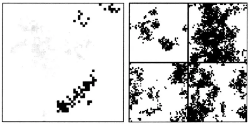
Another way to look at the distribution of diversity is how it is distributed over space. When reproduction is local, nearby individuals tend to be related to each other, and as

Fig.

11

in particular regions. This leads to boundaries between divergent subpopulations. An observer might be tempted to conclude that there are differences in the local conditions on either side of the boundary which caused the population to diverge because the subpopulations on each side have specialized, or that the boundary is due to a barrier to dispersal. Alternately, an observer might conclude that boundary is there because one of the subpopulations migrated from somewhere else. However, these boundaries are a consequence of the local reproduction process only, and do not require selection or unusual historical events in order to form. When inheritance is from multiple parents, each set of traits inherited separately has its own such pattern of diversity.

B 420000 20000 - 10000-0 2W0 5000 0 50000 le+05 t

Figure 10: Diversity in populations, even when they have reached a steady state, under-goes large fluctuations. The plot shows a time series of the diversity of a spatially dis-tributed population. The diversification phase, during which the population approaches

the diversity capacity, lasts roughly until time t = 20, 000 generations. Thereafter, the

average remains constant but there are losses of all sizes up to about 2/3 of the total branch length. The distribution of these losses is shown in Fig. 8. The inset shows that the time series of a well-mixed population is similar.

Figure 11: Simulated spatial pattern of diversity in a two-dimensional space (repre-sented as a lattice of

I

left panel, the individuals shown in grey or black represent a genealogically divergent group whose most recent ancestor in common with the rest of the population (white)

lived about

10,000

di-verged about 2,000 generations ago. The four panels at right show the most divergent groups in the later evolution of the same population (in black, subgroups not

distin-guished), every 2,000 generations starting at t = 20, 000.

U;..

V

U

I

References

[1] R. A. Fisher, The genetical theory of natural selection (Oxford University Press,

London, 1930);

[2] R. Frankham, K. Lees, M.E. Montgomery, P.R. England, E.H. Lowe, D.A. Briscoe,

1999. Do population size bottlenecks reduce evolutionary potential? Anim. Cons. 2, 255-260.

[3] Watterson, G. A. On the number of segregating sites in genetical models without

recombination. Theor. Pop. Biol. 7, 256 (1975).

[4] Watts, D.J., & Strogatz, S.H. (1998). Collective dynamics of "small-world" net-works. Nature 393, 440-442.

Chapter 2: Within-species diversity

-

analytic

and simulation results and comparison with

experimental data'

Abstract

In this chapter we give analytic arguments and simulation results for the results stated in the previous chapter, and investigate additional properties of diversity. We discuss the relevance of our findings to biological systems, and show that two predictions from the model - the number of ancestors of the living population at a given time in the past, and the distribution of uniqueness - agree with existing experimental data on global samples of Pseudomonas bacteria.

The study of diversity is central to biology, and the mechanisms that give rise to the enormous variety found in nature are of great inherent interest. Understanding diver-sity also has practical value for the conservation of biological resources [2] since it is important to the resistance of a population to disease and its adaptability to environ-mental changes [3,4]. DNA sequencing is increasingly being used to probe the genetic structure within species, providing opportunities for comparison with experiment.

The genetic structure of populations has been studied using coalescent theory and related methods [5-9], including studies of subdivided and continuous populations [10,

11], and simulations have been used to study particular models of spatial populations [12]. Here, we focus on the scaling dependence of population properties - including diversity, its distribution in the population, and the sizes of losses of diversity - on key variables such as area and time. The scaling behavior is robust to many variations in the model, and provides predictions that can be compared with experiments. We first present the model in detail and show that properties of diversity can be obtained

by modelling the ancestry of the population as a coalescing random walk. We use this

to derive the distribution of genetic distances between individuals in the population, showing that a spatial population has a power law distribution, which is fundamentally different from well-mixed populations, which have an exponential distribution. By

deriving the scaling of diversity with habitat area, we will demonstrate that area has a stronger effect on within-species diversity than on species diversity. We will then give results for the power law distribution of genetic uniqueness and of the sizes of fluctuations in diversity.

Model. Our lattice model for the population itself is similar to the stepping stone model

[13]. The essential features of spatial populations are locality and a form of competitive

interaction that results in local limitation on density. A step of the simulation consists of the birth of a new generation. At each site, new individuals are born, and we identify the parent of each organism as being either a previous organism at that site, or one at one of the neighbors (Fig. 3 in Chapter 1). Local competition is included by allowing

only a fixed number

nmax

take

nmax

that each organism can be the offspring of any parent in the previous generation (the Wright-Fisher model [14, 15]); the population remains of constant size N.

Mutation will not be included in the model directly; instead, we can superimpose assumptions about mutation on the properties of genealogical trees to obtain genetic diversity. We will first make the assumption of neutrality (that natural selection plays a negligible role); thus, the individual at any site is equally likely to be the offspring of an individual at any connected site in the previous generation. We will then characterize conditions under which selection alters the results. We will also first treat the case where individuals have only one parent, which applies to genes, organelle DNA, and asexual organisms, and then use these results to obtain approximate results for sexual populations.

Genetic distances between individuals. Consider an individual on the lattice at time

T = 0 (the present); we will use T to stand for the number of generations before the

present. The sequence of its ancestors can be traced backward in time, with the parent always located at one of the lattice sites connected to that of its offspring. The sequence of locations of the ancestors of an individual is thus a random walk. Two such walks stepping onto the same site corresponds to two individuals having a common parent;

so, for two individuals x, and X2 at different locations on the lattice, the time until

their common ancestor is distributed as the first intersection time of two random walk-ers. (Other assumptions such as different dispersal distances or migration rates, lattice geometry, overlapping generations and number of occupants per site do not change the scaling properties). If mutations are random, the number of mutations occurring since

the lineages of x, and x2 diverged is binomially distributed with mean proportional to

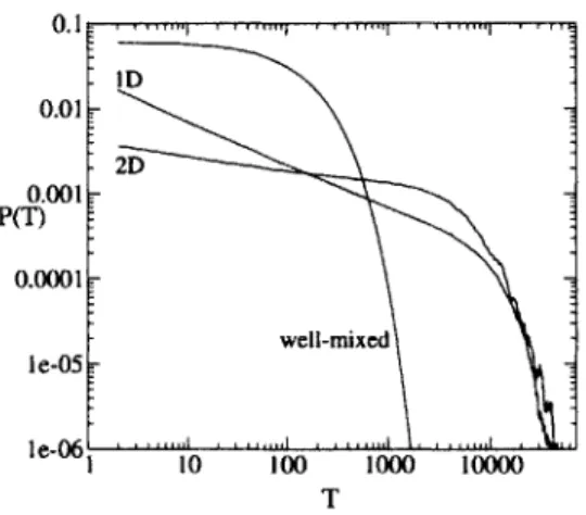
0.11 0.01 -2D 0.001 P( 0.0001 well-mixed I e-05 Ie-06, 10 100 1000 10000 T

Figure

1:

population and a one-dimensional population (L = 150), and the analytic result

P(T) = _( - )T 1 e-T/N for a well-mixed population (N = 150). Here

and in subsequent figures, the two-dimensional lattice size L = 30 unless otherwise

noted.

It is known that in spatial populations a typical pair of individuals is more dis-tantly related to each other than in well-mixed populations [14]. In well-mixed pop-ulations, the number of pairs at a given genetic distance from each other has an ex-ponential distribution [5]. In spatial populations, by contrast, we find that the ge-netic distances have a power law distribution (Fig. 1). In a well-mixed population, there is a probability 1/N of two individuals having the same parent. With probability

1 - -, these individuals did not have the same parent, but with probability (1 -

)

they had the same grandparent; and so on. A(T) is thus exponentially distributed:

A(T) =

y

Shape of the genealogical tree. Now consider the entire population of individuals on

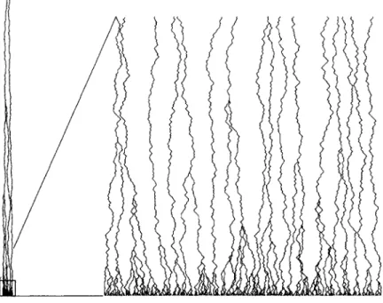
the lattice. The ancestry of this population can be described by a spatial genealogical tree, which we will use to obtain properties of diversity. Fig. 2 shows the genealogical tree of a one-dimensional population. The lineage of each member of the current pop-ulation executes a random walk. Two walkers (lineages) coalesce into one when they collide. The number of lineages L(T) is the number of individuals that lived T gen-erations ago that have descendants in the present. L(T) decreases with time into the past as individual lineages coalesce, and is equal to the number of remaining walkers

Figure 2: Spatial genealogical tree for a one-dimensional population of 300 individu-als. The y-coordinate represents time, with the present generation at the bottom. The ancestors of the current population are shown, with the x-coordinate representing their physical position. At left, the full tree is shown; the common ancestor is 9248 genera-tions before the present. At right, the most recent 300 generagenera-tions are enlarged.

in the coalescing walk. We will derive this function for well-mixed and spatial popu-lations, compare it with experimental genetic data, and then use it to derive the scaling of diversity with habitat area.

The scaling of L(T) in well-mixed populations [15, 16] can be understood as fol-lows. In a genealogical tree, two lineages coalesce if two individuals have the same parent in the previous generation. In the Wright-Fisher model of a well-mixed popula-tion, each lineage can be thought of as jumping to a random site on each time step (time being measured as number of generations before the present), with multiple lineages on the same site coalescing. The number of lineages L(T + 1) in generation T + 1 is therefore the number of distinct individuals in L(T) samples from the set of ancestors

in generation T + 1 with replacement. Let p(T) = L(T)/N be the fraction of

individ-uals in generation T that have descendants in the present. For p(T) sufficiently small (that is, when T is not small) we can neglect all but pairwise coalescence. The

prob-ability that two lineages coalesce into the previous generation is p(T)2 when p(T) is

not large, with a resulting change in p(T) of Ap ~ -p 2/2 (the factor of 1/2 arises

be-cause only one lineage is lost for a pairwise coalescence [17]; still, the scaling behavior

depends only on the proportionality of change to p2 and not on the coefficient), which

in the continuous limit is = -p2/2, giving p(T) = 2, i.e. the scaling behavior:

p(T) ~'

In a spatial population, L(T) can be expressed as p(T)Ad, where d is the popula-tion density, A is the habitat area, and p(T) is the fracpopula-tion of individuals in generapopula-tion

T that have descendants in the present. p(T) is the probability that a given site is

occupied at time T in a coalescing random walk starting with all sites occupied. Ex-pressions for p(T) in different dimensions have been derived [18]; in two dimensions,

p(T) - 1/vi/t and in two dimensions, p(t) ~ log(T)/T. Thus, the scaling behavior of

L(T) with time for a spatial population differs from that of a well-mixed population by

a logarithmic factor, which is a relatively small distinction when compared to the quite different scaling behavior of the distributions of pairwise genetic distances.

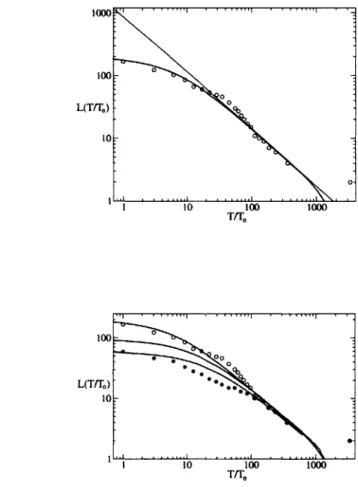
Comparison with experimental data. An experimental test of this model is shown in Figure 3. L(T) was obtained from a clustering analysis of Pseudomonas bacteria

[19] sampled at different sites around the world. The experimental data is long-tailed,

and this tail is well approximated by both the well-mixed and spatial prediction. It is important to emphasize, however, that the original theoretical result is the result expected for the genealogical tree of the entire population rather than a limited set of samples of the population, as was obtained in the experiment. We thus performed

theoretical calculations using simulations (shown in the figure) that directly represented the sampling of the population at specific geographical locations used in obtaining the

Pseudomonas data. To model the sampling of the population, we directly represented

the organisms at the specific geographical locations where the Pseudomonas samples were obtained. In the simulations, lattice cells represent a physical region of the earth. 248 lineages were placed at sites whose cells contain the latitude/longitude coordinates of the 248 samples in the Cho and Tiedje data. At each step of the simulation, moving backward in time, a lineage performs a random walk staying in place or moving to a neighboring site. At its destination, with a certain probability pc, it coalesces with other

lineages at that site. Pc and the number of simulation time steps NT corresponding to

one unit To of biological time, as well as the lattice size, are adjustable parameters. The parameters were set by a simple fitting procedure that adjusts the intercepts of

L(T) at the L and T axes but does not affect the shape of the curve. The parameters

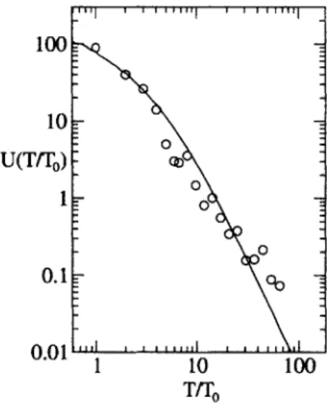
were adjusted to simultaneously fit both L(T) and a different property of the same genealogical tree: the distribution of genetic distinctiveness, that is, the number U(T) of samples whose most closely related sample diverged from it T generations ago, as described below. No special allowances were made for earth curvature or topography (e.g. oceans) that might affect the last few points, which represent global dispersal of only a few most ancient lineages. The result is the solid line in Fig. 3.

To understand this curve, we note that the deep part of the genealogical tree (long times) corresponds directly to the scaling result given for the full population (thin line in Fig. 3). This result is consistent with the recognition that the samples taken from all over the world should be a complete representation of the deepest part of the ge-nealogical tree. An extrapolation of this curve to T/To = 1 gives a rough estimate of the total diversity of the population, in terms of the number of genotypes that could be

distinguished at the level of resolution of the data (a genomic similarity value r = .95),

suggesting on the order of 1,000 genotypes. For the part of the curve corresponding to recent times, the sampling should underrepresent the number of lineages in the ge-nealogical tree. This can be seen the figure as values of L(T) which are lower than the scaling result for the full population for short times. The degree to which the sampling underrepresents the tree, however, depends on the spatial structure of the population. Although a simulation of a well-mixed population also matches the data from sam-ples taken from around the world, it does not match a spatially correlated sub-sample. The lower data points (diamonds) in Fig. 3 correspond to a sub-sample consisting of the samples taken in California. A comparison with what would be expected for a completely mixed population (dotted line in Fig. 3) shows it is inconsistent with the experimental results for the spatially correlated sampling. Therefore, the overall

(a) 1000 0 L(T/To) 10: io0-I10 100 1000 T/1O (b) 0 L(Tfr,) *e.

10-Figure 3: (a) Number of lineages as a function of time in the past L(T), comparing experimental data (circles) and a spatial simulation of the sampled population (solid line). The dotted line corresponds to theory for the whole population. The L-intercept of this line provides a rough estimate of the genetic diversity of the entire population, that is, on the order of 1000 genotypes that could be distinguished at the level of reso-lution of the data. (b) A comparison of the spatial and well-mixed cases. L(T) for a subset of the sampled population consisting of the samples from one geographic region is shown as stars, with a comparison of a spatial (dashed line) and well-mixed (dotted line) simulation of the subset. The experimental data (circles) and simulation (solid line) for the full population is as in part (a). The spatial simulation matches the data for the spatially correlated sample more closely, indicating the importance of spatial structure. Experimental data was obtained from Cho and Tiedje [19]. Time T in the

past (the current generation being at T = 0) is normalized by dividing by To, the time

to the smallest genetic difference considered. The number of simulation time steps NT corresponding to one unit To of biological time is 160 and the coalescence probability

diversity of the California samples is lower than it would be if the population were well-mixed. A spatial simulation of the ancestry of the California samples alone, using the same parameters as for the full simulation, matches the experimental data for the California samples. This effect of correlated spatial sampling occurs only for the case of a spatially structured population, and not for a well-mixed population where local samples and random samples would be equivalent. The results confirm the importance of spatial structure to the Pseudomonas global population. The results of spatial theo-retical calculations closely match the experimental data over its full range. Details of our method are given in the appedix.

Scaling of diversity with area. Area is an important factor in biodiversity. The area of habitat available to organisms has been found to be a primary determinant of their diversity above the species level, as measured by the number of species [20, 21]. Ex-perimental results have found that the number of species S in a sample area A scales

as S = AZ on most scales, with z typically 0.25 and ranging from 0.15 to 0.4 [20,21].,

and this scaling has been modelled theoretically [20,22]. We will now use the scaling of L(T) to derive the scaling of the total diversity within a population. Geographically limited dispersal has been found to increase diversity in many species [23] (includ-ing human Y-chromosome [24] and mitochondrial DNA [25]). Geographic differen-tiation has been found in viruses [26], bacteria [19], plants [27], trees [28], inverte-brates [29], amphibians [30], mammals [31] and birds [32], both in two-dimensional

and one-dimensional [33] habitats.

Every parent-offspring link in the ancestry of the living population represents a chance for mutation. Therefore, diversity is a function of the total length of all branches of its spatial genealogical tree. A key difference between species diversity, as measured

by the number of species, and genetic diversity is that the former treats all species as

equally distinct, not considering the degree to which species are different from each other. The measures used in this paper, by contrast, count additional mutations along a lineage that make a descendant progressively more different from its ancestor and relatives.

We can obtain the branch length B by summing the number of lineages over all generations in the past up to the expected time TA of the most recent common ances-tor of the population. Any mutations that occurred before the most recent common ancestor will be shared by the whole population and will not contribute to diversity. Thus,

B =ZTA L(T).

set-ting L(TA) = 1. Any individuals that do not have descendants in the present are not

counted in B, thus excluding mutations that have become extinct. Under the assump-tion that the same mutaassump-tion is not likely to arise more than once in the ancestry of the population (sometimes known as the "infinitely many sites" assumption), the genetic diversity measured as the total number of distinct mutations is proportional to B. If this assumption does not hold, we must ensure that mutations that are found more than once in the tree are counted only once; thus the expected number of distinct mutations

in the population is D(B) =a " (1 - e-LB), where 1 is the per-genome mutation rate

and pL is the probability of a particular mutation arising at a particular locus. (This is akin to the Jukes-Cantor correction for estimating the divergence time between two

sequences, but in reverse [34]). Fig. 2 in Chapter

1

proportional to branch length for a range of plausible mutation rates, but saturates for high mutation rates (or small genomes).

In two dimensions, L(T) is proportional to A* I , implying that TA scales as

A log(A), so the branch length scales as:

B(A) ~ A[log(A) + log(log(A))]2 - A(log(A))2

Thus, for a two-dimensional habitat, B grows somewhat faster than area, but by a

relatively slowly increasing factor of log2(A). Still, this implies a much faster increase

with area for genetic diversity than has been measured for species diversity. Fig. 6

in Chapter

1

simulated population.

We can also consider an effectively one-dimensional habitat, whose topology cor-responds to a number of natural habitats such as rivers and coastal or tidal zones, if the width of the habitat is not much more than the dispersal distance. In one dimension,

L(t) ~ .The expected time of the most recent common ancestor TA ~ A2, and so the branch length scales as:

B(A) ~ A L' dT ~ A2

Thus the total branch length in one dimension grows much faster than length or pop-ulation size; it quadruples when length or poppop-ulation size is doubled [35]. This is different from well-mixed populations, whose diversity scales as N log N, where N is the population size [5].

These results assume that dispersal occurs to a neighboring site. When there is

longer-range dispersal (e.g. with Gaussian dispersal distances), and local populations

be expected, as long as the dispersal distance is significantly smaller than the size of the habitat. This was confirmed by simulations. When some dispersal happens at long distances, a transition between spatial and well-mixed behavior is expected.

The above has also assumed that there is no recombination; in sexual populations, the tree for different portions of the genome (such as genes and organelle genomes) may be different. However, the diversity-area relationship is essentially the same in sexual and asexual populations. To illustrate the effect of recombination, consider the following hypothetical extreme case: each individual has g separately inherited units of the genome, each inherited independently from a random neighboring individual in the previous generation without linkage. Each unit has its own genealogical tree, and total diversity is the sum of the contribution of each unit. Thus, the total is the same as in an asexual population with the same per-genome mutation rate [36].

Another measure of diversity is the average genealogical distance between individ-uals, sometimes known as nucleotide diversity [37]. In nonspatial and spatial popu-lations alike, the scaling of this quantity is the same as the scaling of the most recent common ancestor of the whole population. In a well-mixed population, the average

ge-nealogical distance between members of the population is Aavg =

fOT

In a spatial population, the average genealogical distance Aavg between members of the population is the first hitting time of a pair of random walkers, averaged over all

walks and pairs of locations. This quantity scales as N2

in one dimension and NlogN in two dimensions [38].

Founding and perturbation. The dependence of diversity on habitat area or

pop-ulation size implies that habitats have a diversity capacity. A poppop-ulation in which mutation and extinction are in balance in the long term will have a long-term average diversity equal to this capacity, though the genetic makeup of the population will be constantly changing. (A similar concept applies to species richness [22]). Diversity may be lower than the capacity of the habitat due to recent founding of the population or to perturbations that kill off part of the population. A population with initially low diversity increases in diversity until its average reaches the diversity capacity. In a spa-tial population, we can assume that the size of the population increases to its long-term average in a time much shorter than TA, the time to most recent common ancestor in a non-perturbed population, since the time to populate an unoccupied habitat scales

as A1/2 in two dimensions (given a uniform rate of spreading) whereas TA scales as

A(log(A))2. (In one dimension the values are A and A2 _{respectively). Given this}

assumption, the genealogical tree looks like that of a non-perturbed population, ex-cept its more distant history is effectively "cut off" by the diversity-reducing or

found-1.2e+06 I e+06 8e+05 B 6e+05 4e+05 2e+05

-5000 I e- 5 1.5e+05 2e+05 2.5e+05

T

Figure 4: Increase in diversity of a one-dimensional population with initially low di-versity, before it reaches its long-term average TA. The dotted line is the analytic result

B (t)~, A Vt.

ing event. Diversity at a time of t generations after the event is B(t) ~'

fL(t)

for t < TA, giving B(t) ~ Avft in one dimension; the fraction of diversity

recov-ered by time t is F(t) = Vt/A. In two dimensions, B(t) ~ A(log(t))2

and the

fraction F(t) = (log(t)/log(A))2

. In a well-mixed population, B(t) ~ Nlog(t) F(t) = log(t)/ log(N). Figs. 4 compares these results to simulations in one

dimen-sion, and Fig. 5 in Chapter

1

increase proceeds rapidly but it slows down with time, and continues until full recov-ery at time t = TA. Whether events that cause the loss of most of a population's diversity affect its long-term average diversity therefore depends on the frequency of such events relative to TA; if the time between events is large compared to the recovery time, they will not decrease the long-term average. Diversity may also be higher than the capacity of the habitat, as when a population is restricted in range to part of its original habitat or moved to a smaller one. Though the diversity may remain high in the short term, it will eventually decrease to the capacity of the smaller habitat.

Effect of selection. Selection can impact diversity in at least two ways. Spatially vary-ing selection (that is, local adaptation) favors different genotypes in different parts of the habitat. This causes barriers to dispersal which will tend to increase the diversity of the whole population, though it may decrease diversity in a local area. On the other hand, spatially uniform selection, in which particular mutants can have higher fitness anywhere in the habitat, can decrease diversity, since the descendants of a mutant can take over the population in a short time, thus wiping out the population's existing diver-sity before an equivalent amount of diverdiver-sity has had time to develop in the descendants of the mutant. (This is known as periodic selection or genetic hitchhiking [39,40]). We

define a periodic selection event to be one where the descendants of a mutant take over the population in a time less than the recovery time TA, and denote the rate of such mutations arising in an individual as AR. (Mutations that take on the order of TA generations are not distinguishable from neutral mutations.) Whether periodic selec-tion affects the long-term average diversity therefore depends on the frequency of such

selected mutants arising relative to the recovery time TA; if the time tE = 1/uRN

is large compared to TA, average diversity will be systematically reduced. As area increases, both N and TA increase (larger populations require longer to recover their diversity), so A may reach a size at which selection causes the rate of increase in di-versity with area to slow. A first approximation for the reduced didi-versity when the

time between events is smaller than the recovery time is B(t = tE), where B(t) is

the diversity at t generations after a founding event, giving B - A[log( 1 )]2 in two

dimensions; more rigorous and comprehensive results for well-mixed populations are given in Ref. [39].

Distribution of diversity and its fluctuation. Unlike the result on relatedness, which

allows us to distinguish well-mixed and spatial populations, the following results are similar for both well-mixed and spatial populations, illustrating their highly robust (uni-versal) nature. The uniqueness u(i) of an individal, which we use to quantify how di-versity is distributed within the population, is defined as the number of generations to

i's most recent common ancestor that has another currently living descendant. The

mu-tations that took place since that ancestor are not shared with any other member of the population. Since the probability distribution P(u) is a power law (Fig. 8 in Chapter

1), u has no characteristic size. Its distribution implies that a disproportionate fraction

of the genetic diversity is typically contained in a small fraction of the population. This distribution can be understood as follows. The probability P(U > u) that an individual has uniqueness greater than u is the probability that its lineage, traced backward through time, never exists on a site that has another lineage for all T < u. In the well-mixed model, the probability that no other lineage jumps to a particular site is:

(-_)p(T)N t-- exp(-p(T))

p(T) is approximately A, with a measured from simulations of p(T) to be 1.95, and expected analytically to be 2. This gives:

P(U > u) flu= exp(-g) = exp(-a 2 F 1

)

Thus the exponent depends on the coefficient a of the scaling of p(T). The probability

density is P(u) = - , giving:

P(u) ~ U-ai u -- 2.95,

consistent with both the well-mixed and spatial simulations of P(u).

The scale-free distribution of uniqueness also applies to subgroups defined by a

given

level

of its ancestor T. generations ago. We define the uniqueness ug of the group to be the uniqueness of the ancestor. The genealogical tree of the ancestors of these groups have the same properties as that of the present population of individuals, only starting with a smaller initial value of L(T). Thus, their uniqueness follows the same power-law distribution.

In Fig. 5, we compare these results to experimental data. The above distribution applies to the whole population. Sampling changes the distribution by making it longer-tailed, corresponding to a greater proportion of individuals which are more unique with respect to the sampled population. We obtained U(T), the number of samples whose genetic distance to their most closely related sample is T, from the same genetic data as in Fig. 3. Fig. 5 compares this distribution with a simulation of U(T) for a sampled spatial population. By adjusting the parameters of the simulation, we simultaneously fit both U(T) and L(T); the simulation is in good agreement with experimental data using the same simulation parameters as in Fig. 3.

In sexual populations, uniqueness is the sum of u(i, g) over all genes g. Figure 9 in Chapter I shows the distribution of uniqueness for sexual populations for different numbers of independently inherited units. Summing the uniqueness of these multi-ple units changes the shape of the distribution, making smaller values of u rarer, and medium values of u more common relative to large ones. However, the long-tailed, power-law character of the distribution remains, and very divergent individuals can still occur in the power-law tail. For the figure we use the simplifying assumption that each unit is independently inherited from a random connected site. Each can actually only be inherited through one of two parents, which correlates the trees with each other, and genes are not inherited independently because of linkage, so the actual change in the shape of the distribution is not as great.

Diversity is often characterized using measures such as Wright's FST [41], which measures the degree of differentiation between subpopulations relative to the diversity of the whole population. However, the unevenness of the distribution of genetic diver-sity among individuals is not adequately captured by FST. Divergent individuals and groups do not necessarily correspond to geographically isolated populations, and if a