HAL Id: hal-01457630
https://hal.archives-ouvertes.fr/hal-01457630
Submitted on 23 May 2018
HAL is a multi-disciplinary open access
archive for the deposit and dissemination of
sci-entific research documents, whether they are
pub-lished or not. The documents may come from
teaching and research institutions in France or
abroad, or from public or private research centers.
L’archive ouverte pluridisciplinaire HAL, est
destinée au dépôt et à la diffusion de documents
scientifiques de niveau recherche, publiés ou non,
émanant des établissements d’enseignement et de
recherche français ou étrangers, des laboratoires
publics ou privés.
Tropical climates at the Last Glacial Maximum: a new
synthesis of terrestrial palaeoclimate data. I. Vegetation,
lake levels and geochemistry
Isabelle Farrera, Sandy P Harrison, I Colin Prentice, Gilles Ramstein, Joel
Guiot, Patrick J Bartlein, R Bonnefille, M Bush, Wolfgang Cramer, U
Grafenstein, et al.
To cite this version:
Isabelle Farrera, Sandy P Harrison, I Colin Prentice, Gilles Ramstein, Joel Guiot, et al.. Tropical
climates at the Last Glacial Maximum: a new synthesis of terrestrial palaeoclimate data. I.
Vege-tation, lake levels and geochemistry. Climate Dynamics, Springer Verlag, 1999, 15 (11), pp.823-856.
�10.1007/s003820050317�. �hal-01457630�
Climate Dynamics (1999) 15 : 823}856 ( Springer-Verlag 1999
I. Farrera
' S. P. Harrison ' I. C. Prentice ' G. Ramstein
J. Guiot
' P. J. Bartlein ' R. Bonne5lle ' M. Bush ' W. Cramer
U. von Grafenstein
' K. Holmgren ' H. Hooghiemstra ' G. Hope
D. Jolly
' S.-E. Lauritzen ' Y. Ono ' S. Pinot ' M. Stute ' G. Yu
Tropical climates at the Last Glacial Maximum:
a new synthesis of terrestrial palaeoclimate data.
I. Vegetation, lake-levels and geochemistry
Received: 7 September 1998 / Accepted: 18 March 1999
Abstract Palaeodata in synthesis form are needed as
benchmarks for the Palaeoclimate Modelling
Inter-comparison Project (PMIP). Advances since the last
synthesis of terrestrial palaeodata from the last glacial
maximum (LGM) call for a new evaluation, especially
of data from the tropics. Here pollen, plant-macrofossil,
lake-level, noble gas (from groundwater) and
d18O
(from speleothems) data are compiled for 18$2 ka
(
14C), 32
3N}33 3S. The reliability of the data was
evalu-I. Farrera
Laboratoire PaleHoenvironnements et Palynologie, USTL, Place Eugene Bataillon, F-34095 Montpellier ceHdex 5, France S. P. Harrison1 ( ) ) I. C. Prentice2 ) D. Jolly1,2
Max Planck Institute for Biogeochemistry, PO Box 10 01 64, D-07701 Jena, Germany
Also at:
1Dynamic Palaeoclimatology, Lund University, Box 117, S-221 Lund, Sweden
2School of Ecology, Lund University, Ecology Building, SoKlvegatan 37, S-223 62 Lund, Sweden
G. Ramstein ) U. von Grafenstein3 ) S. Pinot
Laboratoire des Sciences du Climat et de l'Environnement, CEA Saclay, Ba(timent 709, Orme des Merisiers,
F-91191 Gif-sur-Yvette ceHdex, France
Also at:
3Geologie TU MuK nchen, Lichtenbergstra{e 4, D-85747 Garching, Germany
J. Guiot
IMEP CNRS, Case 451, FaculteH de St JeHro(me, F-13397 Marseille ceHdex 20, France
P. J. Bartlein
Department of Geography, University of Oregon, Eugene, OR 97403, USA
R. Bonne"lle
Palynology Laboratory, French Institute of Pondichery, 11 St. Louis Street., P.B. 33, Pondicherry 605 001, India M. Bush
Department of Biological Sciences,
Florida Institute of Technology, 150 West University Boulevard, Melbourne, FL 32901, USA
ated using explicit criteria and some types of data were
re-analysed using consistent methods in order to derive
a set of mutually consistent palaeoclimate estimates of
mean temperature of the coldest month (MTCO), mean
annual temperature (MAT), plant available moisture
(PAM) and runo! (P-E). Cold-month temperature
(MAT) anomalies from plant data range from !1 to
!
2 K near sea level in Indonesia and the S Paci"c,
through !6 to !8 K at many high-elevation sites
W. Cramer
Potsdam Institute for Climate Impact Research (PIK),
Telegrafenberg, P.O. Box 60 12 03, D-14412 Potsdam, Germany K. Holmgren
Department of Physical Geography, Stockholm University, S-106 91 Stockholm, Sweden
H. Hooghiemstra
Department of Palynology and Paleo/Actuo-ecology, University of Amsterdam, Kruislaan 318,
NL-1098 SM Amsterdam, The Netherlands G. Hope
Research School of Paci"c Studies,
Australian National University, Canberra 0200, ACT, Australia
S.-E. Lauritzen
Department of Geology, University of Bergen, AlleHgaten 41, N-5007 Bergen, Norway Y. Ono
Laboratory of Geoecology, Graduate School of Environmental Earth Science,
Hokkaido University, Sapporo 060, Japan M. Stute
Lamont-Doherty Earth Observatory, Route 9W, Palisades, NY 10964, USA
G. Yu1
Nanjing Institute of Geography and Limnology, Chinese Academy of Science, Nanjing 210093, China
Also at:
1Dynamic Palaeoclimatology, Lund University, Box 117, S-221 Lund, Sweden
to !8 to !15 K in S China and the SE USA. MAT
anomalies from groundwater or speleothems seem
more uniform (!4 to !6 K), but the data are as yet
sparse; a clear divergence between MAT and
cold-month estimates from the same region is seen only in
the SE USA, where cold-air advection is expected to
have enhanced cooling in winter. Regression of all
cold-month anomalies against site elevation yielded an
estimated average cooling of !2.5 to !3 K at
mod-ern sea level, increasing to +!6 K by 3000 m.
How-ever, Neotropical sites showed larger than the average
sea-level cooling (!5 to !6 K) and a non-signi"cant
elevation e!ect, whereas W and S Paci"c sites showed
much less sea-level cooling (!1 K) and a stronger
elevation e!ect. These "ndings support the inference
that tropical sea-surface temperatures (SSTs) were
lower than the CLIMAP estimates, but they limit the
plausible average tropical sea-surface cooling, and they
support the existence of CLIMAP-like geographic
pat-terns in SST anomalies. Trends of PAM and lake levels
indicate wet LGM conditions in the W USA, and at the
highest elevations, with generally dry conditions
else-where. These results suggest a colder-than-present
ocean surface producing a weaker hydrological cycle,
more arid continents, and arguably
steeper-than-pres-ent terrestrial lapse rates. Such linkages are supported
by recent observations on freezing-level height and
tropical SSTs; moreover, simulations of &&greenhouse''
and LGM climates point to several possible feedback
processes by which low-level temperature anomalies
might be ampli"ed aloft.
1 Introduction
The climate of the last glacial maximum (LGM)
con-tinues to present challenging problems for
palaeo-climatologists and climate modellers, now nearly
20 y after the publication of Peterson et al.'s (1979)
pioneering synthesis of terrestrial palaeodata and the
CLIMAP (1976, 1981) reconstruction of conditions at
the ocean surface. In some ways, our ignorance of the
processes determining the nature of the glacial climate
regime appears to have grown since then. The
exis-tence of ice-core records and the resulting discovery
of major changes in the atmospheric concentrations of
the greenhouse gases CO2, CH4 and N2O between the
LGM and Holocene has presented new, unsolved
prob-lems about the regulation of natural changes in global
biogeochemical cycles, their linkages to one another
and their coupling with the physical climate system
(Lorius and Oeschger 1994). The discovery of rapid
climate changes during the last glacial period
chal-lenges our ability to predict the coupled physical
dy-namics of atmosphere, ocean and ice (Johnsen et al.
1992; Bond et al. 1993; Broecker 1997). The need to
understand the processes which bring about major
state changes in the Earth's climate is made clear by
atmosphere-ocean model simulations showing that
there are complex transient e!ects in the response of
climate to anthropogenic changes in greenhouse gas
budgets (Rahmstorf 1994; Stocker and Schmitter 1997),
and suggest a potential for further feedbacks on
atmo-spheric carbon dioxide concentration [CO2]
(Sar-miento and le QuereH 1996; Sar(Sar-miento et al. 1998).
A focus on the tropics, in particular, is justi"ed by the
current debate about the e!ectiveness, or otherwise, of
homeostasis in tropical temperatures when forced by
changes in [CO2] (Kattenberg et al. 1996). If we are
able to reconstruct and successfully model the climate
response of the tropics at the LGM, we will have reason
to be more con"dent in our ability to estimate the
global climate sensitivity to changes that may be
brought about by human actions.
Several scienti"c developments since the Peterson
et al. (1979) synthesis have greatly increased the
amount of information available on the state of
di!er-ent aspects of the Earth system at the LGM. They
include:
1.1 LGM boundary conditions
These can now be speci"ed with greater con"dence and
precision than was possible when the "rst simulations
of LGM land climates were performed (Williams et al.
1974; Gates 1976; Manabe and Hahn 1977; Manabe
and Broccoli 1985a, b; Broccoli and Manabe 1987;
Kutzbach and Guetter 1986). We now have a globally
consistent reconstruction of ice distribution and
rela-tive sea-level changes from the LGM to present (Peltier
1994); measurements of LGM atmospheric
concentra-tions of the major greenhouse gases (Barnola et al.
1987; Chappellaz et al. 1990; Leuenberger and
Sigen-thaler 1992); and a better speci"cation of LGM
insola-tion forcing following the discovery that the
14C age of
18 ka for the LGM represents+21 ka in astronomical
years (Bard et al. 1990; Kutzbach et al. 1993).
1.2 Palaeoclimate modelling
This has advanced considerably, due to the availability
of faster computers and the progressive re"nement of
atmospheric and ocean models. Palaeoclimate
simula-tions with atmospheric general circulation models
are now commonly performed for 510 annual cycles,
and often include interactive oceanic components.
The achievable spatial resolution in global models has
improved to 2}33, and representations of
land-atmo-sphere
interactions
have
become
more
realistic
(Houghton et al. 1996). Simulations including coupling
to dynamical ocean models (e.g. Kutzbach and Liu
1997; Hewitt and Mitchell 1998) and biosphere models
(e.g. Foley et al. 1998) can now be undertaken. In
addition, simpli"ed, lower-resolution but fast models
are being developed that show promise in elucidating
the long-term interactions of di!erent components of
the climate system (Ganopolski et al. 1998). The
gener-ality of model results can be assessed thanks to the
Palaeoclimate
Modeling
Intercomparison
Project
(PMIP) (Joussaume and Taylor 1995; Joussaume et al
1998; Pinot et al. this volume), which has speci"ed
a small number of standard model experiments for 6 ka
and 21 ka that are being carried out by about 20
modelling groups.
1.3 Acquisition of terrestrial palaeodata from the LGM
This has continued, and in particular there have been
major e!orts to obtain records from sediment cores in
previously data-sparse regions in the tropics. Dating
accuracy has also improved thanks to the increasing
use of AMS for
14C-dating small samples of material of
identi"ably terrestrial origin (e.g. plant macrofossils),
thus avoiding the problems of dating sediments mostly
devoid of carbon.
1.4 Data syntheses
These have been carried out on a more comprehensive
and rigorous basis than before, starting with the Global
Lake Level Data Base (Street-Perrott et al. 1989) and
the regional pollen and lake-level data compilations
carried out within the COHMAP project (Wright et al.
1993) and continuing through the IGBP-sponsored
BIOME 6000 project (Prentice and Webb 1998), which
includes the compilation of pollen records for the LGM
and their translation into palaeobiomes using a
stan-dard methodology (Prentice et al. 1996; Prentice, Jolly
and BIOME 6000 participants, unpublished data).
1.5 Understanding and interpretation of the &&classical''
data sources
This has improved greatly. Di!erent types of data
often respond to di!erent seasonal aspects of climate,
and such di!erences may account for apparent
discrep-ancies between proxies (e.g. the coexistence of high lake
stands with steppe vegetation in the Mediterranean
region at LGM: Prentice et al. 1992a). Calibration
methods using multiple data sets have been developed
(Guiot et al. 1993). Possible e!ects of CO2 on treeline
elevations (Street-Perrott 1994; Crowley and Baum
1997; Street-Perrott et al. 1997) have been recognized
and included in ecosystem models (Jolly and Haxeltine
1997). Interpretation of changes in equilibrium-line
altitude (ELA) of glaciers is understood to require
con-sideration of precipitation changes as well as
temper-ature changes (Zielinski and McCoy 1987; Hostetler
and Clark 1997), and observational and modelling
studies of recent glacier variations have suggested the
existence of feedbacks that may amplify the response of
ELA to temperature changes at sea level (Oerlemans
1986; Crowley and Kim 1996; Diaz and Graham 1996;
Crowley and Baum 1997; Martin et al. 1997).
1.6 New data sources
These have been developed, including the &&noble gas
thermometer'' in groundwater (Stute et al. 1992; Stute
and Schlosser 1993) and
d18O in speleothems
(Laurit-zen 1993, 1996) as records of mean annual (subsurface)
temperatures on land.
1.7 Our understanding of the temporal context
of the LGM
This has changed drastically, due to the recognition of
large synchronous climate #uctuations during the
gla-cial stages in high-resolution climate records from
Greenland ice (Johnsen et al. 1992; Dansgaard et al.
1993), marine foraminiferal records (Bond et al. 1993),
terrestrial pollen records (Grimm et al. 1993; Watts
et al. 1996) and loess (Porter and An 1995; Guo et al.
1996; Chen et al. 1997). This context makes it important
to consider the relative response times of di!erent types
of data, and to avoid the mistake of correlating LGM
with short-lived cold episodes, such as the last Heinrich
event (H1) in the North Atlantic. Thus, the selection of
data to correspond to the LGM should be based on
independent dating, and not simply on locating the
most extreme conditions during the much longer
peri-od correlative with isotope stage 2.
1.8 Our purpose
Against this background, we "nd it timely to present a
new synthesis of the available palaeoclimatic data from
terrestrial records at the LGM. We focus on the region
between 32 3N to 33 3S, because of the continuing
inter-est in the problem of reconciling terrinter-estrial and marine
records from the tropics (Webster and Streten 1978;
Rind and Peteet 1985; Anderson and Webb, 1994;
Guilderson et al. 1994; Thompson et al. 1995; Broecker
1997) and because of the key importance of the tropical
temperature response in discussions about future
cli-mates (Houghton et al. 1996). The choice of latitudinal
limits beyond the tropics (sensu stricto) enabled us to
include important data points from the subtropics.
We de"ne the LGM by a
14C-age bracket of
18$2 ka. Although this period was clearly not
climat-ically homogeneous, the independent dating control on
most records is insu$cient to allow greater precision
while the $2 ka tolerance range is narrow enough
to exclude the largest anomalies, namely the Heinrich
events that occurred before (H2:+22}21 ka
14C) and
after (H1: +15-14 ka
14C) the LGM (Bond et al. 1993).
This chronological criterion is applied strictly. Thus,
we do not consider data from other times during
iso-tope stage 2 as representing the LGM. This is an
important di!erence between our approach, which is
oriented towards comparison with model results (Pinot
et al. this volume) for a speci"c time period, and some
discussions in the literature which have focused on the
question of the maximum degree of cooling during the
entire last glacial interval (e.g. Colinvaux et al. 1996).
We insist on the distinction because the LGM as
de-"ned in terms of global ice volume does not necessarily
coincide with the timing of maximum cooling (or even
local glacier advance) in any particular region. If data
were aggregated from a broader time interval, the result
might be a composite of diachronous climates and
might therefore correspond to no physically possible
state of the global climate system.
Our principal aim has been to assemble the extant
information on tropical terrestrial palaeoclimates at
the LGM from the approximately 200 sites that fall in
the geographical and temporal ranges speci"ed, and
to extract where possible quantitative estimates of the
di!erence between LGM and present climate.
Geo-chemical or statistical methods have been used to
re-construct climatic di!erences at a limited number of
sites; these reconstructions were accepted without
modi"cation provided they met certain standards.
More often indirect estimates have been made, e.g.
based on converting elevation shifts of vegetation zones
to changes in temperature. We re-evaluated these
in-direct estimates, based on the originally published data,
using a standard methodology including an objective
method to estimate lapse rates. Estimates of aspects of
the water balance (plant-available moisture and
pre-cipitation minus evapotranspiration) were also
com-piled, but on a qualitative basis.
2 Potential sources of information on tropical palaeoclimate
Many data sources could potentially be used to reconstruct tropical palaeoclimates. No one source has all the characteristics to make it ideal: wide spatial distribution, high temporal resolution, good dat-ing control, direct and well-understood climatic controls, and the potential to yield quantitative climate reconstructions. Furthermore, since individual types of data respond to di!erent seasonal aspects of the climate, multiple types need to be used when reconstructing past climates. The use of multiple types of data also makes it possible to check whether reconstructions based on individual types are phys-ically consistent. The data sources used here are pollen and plant macrofossil records; geochemical and isotopic records from fossil water or carbonates; and lake-level reconstructions based on geomorphic and stratigraphic records. A new synthesis of glacial ELA reconstructions from geomorphic records in tropical mountain regions in underway, and will be reported in a subsequent study (Part II). In the following section we describe the characteristics of each data type in turn, and its relationship to climate.2.1 Pollen and plant macrofossil data
Pollen grains are quantitatively preserved in mire and lake sedi-ments that can be dated by14C. Pollen data are the largest and most widespread source of information on Late Quaternary palaeoen-vironments. Despite di!erences in the production and dispersal of pollen from di!erent plant taxa, pollen assemblages from sediments can be interpreted as a quantitative record of the surrounding vegetation (Prentice 1988). Regionally dominant taxa are normally well represented and smaller counts of less abundant taxa provide additional information, allowing pollen assemblages to be assigned correctly to biomes (Prentice et al. 1996). Procedures to assign biomes, and to make palaeoclimate estimates, can be calibrated using the large sets of pollen data in modern (surface) samples that have been assembled for many regions (e.g. Guiot 1990; Cheddadi et al. 1996; Jolly et al. 1998b; Yu et al. 1998)
Most pollen grains are identi"able to genus or family. Plant macrofossils can often be identi"ed to species. Macrofossils are preserved in some sediments and can provide additional informa-tion, for example by distinguishing climatically indicative species within widely distributed genera (Jackson et al. 1997). Macrofossils are abundant in middens made by Neotoma (packrats) or Hyrax in arid regions. Such middens are 14C-datable and provide a rich source of information on Late Quaternary palaeoenvironments (Van Devender et al. 1987).
Plant taxon and biome distributions are highly sensitive to several aspects of the atmospheric environment. These geographic distribu-tions can be characterized today in a climate space which globally has at least three dimensions, e.g. the mean temperature of the coldest month (MTCO), total growing-season warmth (indexed by growing degree days above a threshold temperature for growth), and plant-available moisture (PAM) (Woodward 1987; Prentice et al. 1992b; Sykes et al. 1996). (PAM represents the availability of soil moisture to satisfy the plants' demand for evapotranspiration; if PAM is reduced, plant carbon gain is also reduced.) Knowing the biome, or knowing the assemblage of plants and their bioclimatic ranges, one can locate a given palaeoenvironment in this space. Changes in pollen assemblages therefore often give information about changes in more than one climate variable (for example, the e!ects of changes in cold-month temperatures and PAM have di!er-ent and independdi!er-ent e!ects on vegetation). Various techniques are used to make climatic inferences, including qualitative comparisons of plants identi"ed with their modern distributions; quantitative estimates of minimum and maximum changes required to produce a given biome shift; and quantitative palaeoclimate estimates based on statistical calibration of modern pollen samples (transfer-func-tion, modern-analog and response surface techniques: Guiot 1991; Bartlein and Whitlock, 1993).
In tropical mountain regions, comparisons of LGM-age pollen samples with vegetation or modern pollen samples from di!erent elevations have often been used to estimate shifts in the apparent elevation of speci"c forest belts or treeline. The reconstructed shifts in apparent elevation are then multiplied by a lapse rate to yield temperature change estimates. However, since photosynthesis and stomatal conductance are sensitive to atmospheric [CO2], vari-ations in [CO2] can in principle modify the response of plants to climate and therefore constrain the locations of plant distributions in climate space. Biome-level responses can only be inferred by ecosystem modelling based on experimental results at the plant and ecosystem levels because [CO2] is essentially constant spatially today (Walker and Ste!en 1997). Nevertheless, the LGM distribu-tions of plant taxa and biomes in relation to climate may have been modi"ed by low [CO2] (Davis, 1991). Tropical mountain treeline, in particular, is thought to be potentially sensitive to low [CO2]. The trees near treeline exist today under conditions of extremely low primary productivity, due to a combination of year-round low temperatures and a low internal partial pressure of [CO2] (Street-Perrott 1994; Street-(Street-Perrott et al. 1997). If [CO2] were further lowered then primary productivity could become too low to sustain tree growth. One model result indicates that LGM treelines in the
tropics might have been lowered by hundreds of metres due to physiological e!ects of 190 ppmv [CO2], i.e. a lowering of the same order of magnitude as that observed (Jolly and Haxeltine 1997).
Changes in the upper elevational limits of montane forest belts, however, are probably unresponsive to [CO2]. The upper eleva-tional limits of lowland and lower-montane rainforest trees are determined by the fact that these taxa, unlike taxa from higher elevations, have no protection mechanisms against chilling or frost (Woodward 1987). We therefore assume that these limits are con-trolled by MTCO. In the tropics sensu stricto and especially in the wet tropics, MTCO and mean annual temperature (MAT) must be closely correlated because of the relatively low seasonal range of temperatures. In the subtropics these two variables can diverge, e.g. any mechanism that would produce colder winters while not a!ect-ing the other seasons would reduce MTCO considerably more than MAT.
Low [CO2] at the LGM might also have led to &&physiological drought'' since stomatal conductance is generally greater at low [CO2], causing greater transpiration per unit leaf area, and is likely to have favoured plants with the C4 pathway of photosynthesis (e.g. tropical grasses), which concentrate CO2 around the chloro-plasts, over the C3 pathway used by most temperate plants and all trees. These e!ects would not be con"ned to high elevations and might have contributed to a general reduction in PAM, as de"ned here, and an expansion of tropical grasslands at the expense of forests.
2.2 Noble gases in groundwater
The solubility of the noble gases (Ne, Ar, Kr, Xe) in water is temperature dependent. Both solubility and its sensitivity to temper-ature increase with atomic mass (Mazor 1972). As water percolates from the land surface through the unsaturated soil zone during groundwater recharge, the noble gas content of the water equili-brates with that of the air in the soil pore space. Exchange ceases once the water reaches the underlying aquifer. Thus, in principle, the noble gas spectrum of groundwater re#ects the temperature in the unsaturated soil zone at the time and place of recharge (Herzberg and Mazer 1979; Stute and Schlosser 1993). In reality, measured noble gas concentrations are often higher than might be expected given perfect equilibration. This additional component, termed &&ex-cess air'' is most likely caused by #uctuations of the water table, trapping small air bubbles that are then dissolved under increased hydrostatic pressure (Heaton and Vogel 1981). Some of this excess air may subsequently be lost by secondary gas exchange across the water table. The excess air contribution is unknown a priori. How-ever, because excess air di!erentially a!ects the apparent temper-ature reconstructed from the di!erent gases (the greatest e!ect is on the lightest, least soluble Ne, the smallest e!ect on Xe), true noble-gas temperature can be estimated by subtracting an excess air contribution that yields similar temperature estimates (within measurement errors) for all four gases (Stute and Schlosser 1993; Stute et al. 1995).
In con"ned aquifers, isolated from the atmosphere, the ground-water #ows downstream to the discharge area carrying a temper-ature signal imprinted in the recharge area. Typical groundwater #ow velocities in con"ned aquifers are of the order of 1 m y~1. As a result, a 50 km long aquifer many potentially provide a 50 000 y long record of temperatures in the recharge zone. How-ever, small-scale mixing processes (dispersion) which occur during groundwater #ow mean that this record is temporally smoothed. Typical dispersion coe$cients are of the order of 10 to 100 y. Model calculations suggest that, for typical #ow velocities and dispersion coe$cients, the smoothing e!ect at the LGM is of the order of 2000 to 5000 y (Stute and Schlosser 1993).
Radiocarbon provides the only well-established method of dating groundwater. The geochemical evolution of the groundwater must be taken into account in order to derive reliable 14C estimates
(Fontes and Garnier 1979). Comparison of correction models (e.g. Phillips et al. 1989) suggests that errors on the order of $2000 y should be assigned to14C ages on groundwater.
Thus, the &&noble gas thermometer'' can be used to provide quan-titative estimates of changes in mean annual ground temperature in the recharge zone. Ground temperature can be equated with mean annual temperature (MAT), except in regions where seasonal snow cover drastically changes the thermal insulating properties of the surface, which is not a concern for any of the sites used here. Groundwater measurements cannot provide high resolution re-cords, partly because of the smoothing of the climate signal caused by dispersion processes, and partly because of the dating errors, but the estimates are presumably reliable for the glacial-interglacial time scale. A caveat is that because of the inherent averaging, the record may also incorporate information from extreme events within the e!ective averaging period. Another possible uncertainty concerns the location of the recharge zone relative to the sampling site. However, any errors introduced by not knowing the exact location of the recharge zone are probably slight, for two reasons. First, the accuracy of noble-gas temperature estimates for the present day supports the reliability of estimates for the past. Second, any possible error due to incorrectly specifying the elevation of the recharge zone is strongly compensated for by the opposing e!ects of atmospheric pressure and temperature on the solubility of noble gases.
2.3d18O in speleothems
Speleothems (stalactites, stalagmites, dripstone) are secondary cal-cium carbonate deposits, precipitated in caves. Speleothem growth is favoured when there is adequate precipitation to produce seepage water and when the ground surface is vegetated so that this seepage water is carbonated, while growth is limited by extreme cold, ex-treme aridity and when the cave is #ooded by water. The isotopic and mineralogical composition of speleothems is determined by the regional climatic and environmental conditions at the time of pre-cipitation. Provided that thed18O of the palaeoprecipitation can be measured, for example in old groundwater, thed18O in the spele-othem carbonate can be used to estimate the absolute cave temper-ature at the time of formation (Hendy 1971; Schwarcz 1986). Cave temperatures are generally stable, approximating to the mean an-nual ground temperature of the region. Speleothems can be precisely dated with the uranium-series method (Schwarcz 1986; Li et al. 1989).
The use of speleothems to reconstruct past climate changes is new and there are few sites from the tropics. Most of these speleothem records have been interpreted as providing estimates of relative changes in various climatic parameters, based for example on an assumed correlation of growth rates with climate (Shaw and Cooke 1986; Brook et al. 1997), or interpretation of isotope excursions either on the assumption that they re#ect single climatic parameters (e.g. Fischer et al. 1996), or by deconvolution of the temper-ature/precipitation signals using information from other data (Hol-mgren et al. 1995; Bar-Matthews et al. 1997; Burney et al. 1997). Lack of independent information on thed18O composition of fossil cave seepage waters has so far prevented the quantitative interpreta-tion of tropical speleothem records except in the single case of Cango Cave in South Africa (Talma and Vogel 1992). We include this record in the present synthesis because it provides an indepen-dent check on the MAT reconstruction from South Africa based on the noble-gas thermometer.
2.4 Lakes
Water-level changes in lakes can occur on a variety of time scales, from intra-annual to geological. The concomitant changes in water depth a!ect many of the physical and biological parameters of the
lake, allowing changes in water level to be inferred from the sedimen-tary or biostratigraphic records preserved in the deposits in or at the margins of lakes (Street-Perrott and Harrison 1985; Harrison and Digerfeldt 1993). Except under exceptional circumstances, when the seasonal changes in the biota or sediments are preserved in the form of annual laminations, lake deposits generally only provide records of the sustained, longer-term (102}104 y) changes in water depth. Such records have been obtained from most regions of the world (e.g. see Street-Perrott et al. 1989; Fang 1991; Yu and Harrison 1995; Tarasov et al. 1996; Jolly et al. 1998a). Changes in water level can be caused by local factors, e.g. damming of the outlet, geomorphic changes causing re-routing of river in#ows, changes in catchment land-use, and tectonism (Dearing and Foster 1986). In general, these factors a!ect only individual lakes. Regionally synchronous changes can be assumed to re#ect changes in the hydrological balance, driven by changes in climate.
Over#owing lakes approach an equilibrium area, such that the sum of runo! from the catchment and the (positive) water balance over the lake surface is balanced by discharge (Szestay 1974; Street-Perrott and Harrison 1985; Mason et al. 1994). Discharge is a mono-tonic function of lake volume; the form of the function depends on the morphometry of the lake and its outlet (Henderson-Sellers 1984). A lake becomes closed (i.e. ceases to over#ow) when the water balance over the lake surface is negative and can therefore alone balance the runo! from the catchment. Generally, lake area and depth vary monotonically with P}E, the (always positive) balance of precipitation and evaporation over the catchment (Cheddadi et al. 1996). Reconstructed changes in lake status (area, depth, or level) can therefore be used to infer the sign of changes in mean annual P}E. Plant-available moisture (PAM) and P}E are estimated indepen-dently, and are not automatically related. In simple scenarios where annual precipitation changes while its seasonality and other factors do not change, both measures must change in the same direction. But there are other possibilities, especially in seasonal climates. For example, increased precipitation in the dry season can be balanced by increased evapotranspiration (promoted by vegetation growth); this would register as increased PAM and no change in P}E. Increased precipitation and decreased evapotranspiration in the already-wet season could conversely produce increased P}E without increasing PAM (Prentice et al. 1992a).
Although lakes usually provide only qualitative records of climate changes, several characteristics make them useful for reconstructing tropical climate changes at the LGM. The climatic controls on the lake water balance are well known (Street-Perrott and Harrison 1985; Cheddadi et al. 1996). Lake records are widely distributed and records of former lakes are common in arid areas. Lake bottom and lake marginal sediments represent a quasi-continuous record of long-term changes, and generally provide material suitable for14C dating.
3 Methods
For each proxy data source, the published literature was surveyed and a listing was made of all of the sites between 32 3N and 33 3S providing either qualitative or quantitative palaeoclimatic informa-tion for the LGM. The LGM was de"ned by a14C-age bracket of 18$2 ka. Site-speci"c information was obtained either from the published articles or from public-access data bases. Although the chronology of every site is based on radiometric methods, the qual-ity of the dating varies between di!erent parts of the record at a single site, between di!erent sites and between di!erent types of records. In addition to giving the total number of dates on which the chronology is based (where this is an appropriate measure of relia-bility), we have also provided an assessment of the quality of the LGM dating control (DC) at each site using the COHMAP scheme (Webb 1985) implemented according to Yu and Harrison (1995). The palaeoclimatic information for each site as given in the original articles is listed systematically. For completeness, Tables 1}4 list all
of the original estimates available at each site, including re-inter-pretations of the proxy data, re-analyses using improved techniques, and multiple studies.
Not all of the palaeoclimatic reconstructions in the published literature are reliable by today's standards. In some cases the under-lying assumptions and methods cannot be identi"ed. Some other reconstructions have been based on incorrect conceptual models, techniques now superseded, or wrong assumptions. We have there-fore closely evaluated individual records, using explicit criteria to assess their reliability. Only sites which meet these explicit criteria are included in the mapped analyses presented later (Fig. 1). In some cases (e.g. the interpretation of changes in vegetation zone elev-ations) we have re-analyzed the original data in order to derive a set of mutually consistent palaeoclimatic estimates. The explicit evalu-ation criteria used for each data source are described below, as are the methods employed in any re-analyses. All of the estimates that we consider reliable, and use in subsequent analyses, are clearly identi"ed in Tables 1}4. Thus, the data as presented in Tables 1}4 make clear wherever we are using an interpretation that deviates from the originally published one, and the underlying logic of our interpretation.
3.1 Estimation of changes in MTCO from pollen and plant macrofossil records
Most of the estimates of tropical temperature changes given in the literature (Table 1) have been obtained by estimating an elevation shift (of one or more climatically sensitive plant species, or of a vegetation zone) and multiplying by a lapse rate, corresponding to an estimate of the rate of decline of temperature with elevation. In some cases the elevation shift has been estimated with some pre-cision, in which case we use a single value as a point estimate; in other cases we know only a minimum, a maximum, or a range. Uncertain-ty is also introduced by the choice of lapse rate. As the relevant temperature here is the temperature near the ground, the lapse rate that applies is the &&terrestrial'' or &&slope'' lapse rate. Although values similar to the free-air moist adiabatic lapse rate (+5 K km~1 at temperatures typical of the lowland tropics) are typically used for this purpose, terrestrial lapse rates can be signi"cantly greater than or less than the moist adiabatic lapse rate. Terrestrial lapse rates can also show large seasonal variations (P.J. Bartlein, J. Guiot, unpub-lished results). Seasonally and locationally dependent terrestrial lapse rates can be estimated statistically by smooth three-dimen-sional interpolation of weather station data on monthly mean tem-peratures.
In the palaeoecological literature the lapse rate used is not always speci"ed, and it is seldom possible to determine whether the value used was an appropriate local terrestrial lapse rate or a generic "gure. Some di!erences between successive estimates (based on the same data), and some di!erences between author's estimates ob-tained from nearby sites, may re#ect varying choices of values for the lapse rate. We have therefore re-estimated changes in MTCO wher-ever these were based on inferred change in the elevations of speci"c vegetation boundaries. In each case we applied a local (modern) terrestrial lapse rate, evaluated at the latitude, longitude and elev-ation of the site, using a data set of long-term monthly mean temperatures from 9176 meteorological stations worldwide (the data set is an updated version of the one used to generate the IIASA data set of Leemans and Cramer 1991). Of these stations, 3346 are located between 32 3N and 33 3S. The lapse rate is calculated as the deriva-tive with respect to elevation of a non-linear function "tted to the monthly data in the space of latitude, longitude and elevation using an arti"cial neural network (Peyron et al. 1988). We distinguish between those sites where the estimated change in MTCO was calculated on the basis of a change in treeline and those for which MTCO was calculated on the basis of changes in forest zones, in order to be able to allow for a possible contribution of [CO2] to treeline changes.
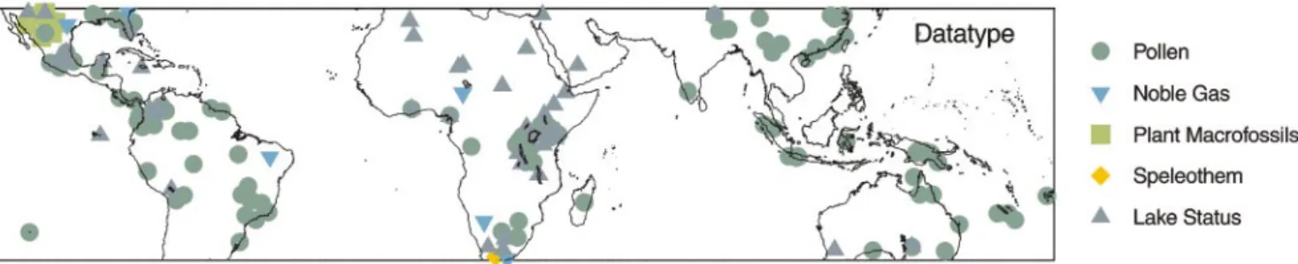
Fig. 1 Distribution of sites, according to data type. This map does not show those sites at which the estimates derived from the litera-ture (listed in Tables 1}4 for completeness) do not match our criteria for reliability and which were therefore not used in subsequent
analyses. Site locations have been shifted by up to a few degrees in data dense areas; however, the location of a given site is the same on each map on which it appears
Fig. 2a+c Anomalies (LGM minus present) of cold-month temper-atures (MTCO) based on pollen data. Maximum and/or minimum estimates based on lapse rate calculations are shown at all sites
where the elevation shift is given in this form d Anomalies of mean annual temperature (MAT) based on noble gas and speleothem data
Table 1 S it es p ro vidin g estimat es o f te mpe rat u re a n d mois tu re -b ala n ce ch an ge s, b a se d o n p ol le n o r p la nt mac ro fo ss il d at a . In fo rm a tio n g ive n in th e o ri g in a l p ub lic a tio n s is g iv en a s A ut h o rs Int er p re ta ti o n ; d a ta u se d in o u r an al yse s a re id en ti " ed a s Thi s w o rk . T he qu ot ed lat itu de , lo n git ude a n d el eva ti o n re fe rs to th e loc a ti o n o f the st udi ed co re o r m idd en si te Au th o r' s int er pre tat io n S ite Cou n tr y Lat . Lon g . E le v. Da ta DC No .14 C S am p ling In ter va l * Tre el in e * Ve g * ¹ an n * ¹ c (3 )( 3 ) (m ) ty pe d a tes res o luti o n (k a ) el ev. zo n e el ev . (3 C) (3 C) No rt h-Am er ic a T w in P eak s U SA 3 1 .97 ! 112 .78 5 6 5 3 7 n /a n /a L at e W is co n si n Cold er H u ec o M ou nta ins U S A 3 1 .90 ! 106 .00 134 0 } 143 0 3 6D 2 #( 14 2 } 12 Goshe n S p ri ng s ; SA 31. 7 2 ! 86 .1 3 1 0 5 1 7 5 ( 12 0 } 6 N o ch an ge Pinckn ey v ille C re ek (PC 1 9 ) U S A 31.5 4 ! 91 .47 7 9 1 2D 1 1 17.5 C old er Pinckn ey v ille C re ek (PC 2 0 ) U S A 31.5 4 ! 91 .48 7 9 1 4D 1 1 18.8 C old er S ier ra Bla n ca ar ea US A 31.1 3 ! 105 .00 143 0 3 2D n /a n /a 18.5 } 11 S tre er uw it z H il ls U SA 3 1 .12 ! 105 .20 143 0 3 4D n /a n /a 18.0 Tun ic a Bayo u (TB 2 3 ) U S A 30.9 6 ! 91 .51 3 1 1 3D 1 1 18.7 C old er Littl e B ayo u S a ra U S A 30.9 5 ! 91 .47 4 9 1 7 n /a n /a W isc o n si n C old er Be n n et t R an ch US A 30.6 2 ! 104 .98 103 5 3 3D n /a n /a 19 } 16 .5 Cam el L ak e U S A 30.2 7 ! 85 .02 2 0 1 7 8 1 3 0 } 14 M a ra vill as Ca ny on US A 29.5 5 ! 102 .90 6 1 0 3 6 D 2 #( 12 9 } 11 S h ee la r L ak e (C a n d D ) U S A 2 9 .52 ! 82 .00 5 1 1 2D 8 ' 1 23.8 } 18 .5 Cold er B ig B en d G ene ral U S A 2 9 .40 ! 103 .75 8 5 0 } 120 0 3 4D n /a n /a 21 } 15 Burr o M es a U S A 29.2 7 ! 103 .40 120 0 3 4D n /a n /a 18.0 Rio G ra n d e Vi llag e US A 29. 2 3 ! 105 .25 6 1 0 } 760 3 1 D n /a n /a 2 3 } 11 Lak e Tu lan e US A 27. 5 9 ! 81 .50 3 6 1 2C 16 ' 12 0 } 17 C entra l & So ut h A m eri ca C u at ro Ci en eg as (F ) M ex ic o 2 7 .00 ! 104 .00 7 4 0 1 1 D 4 ' 1 M id -W is co nsi n n o ch an ge Cua tr o C ie n eg a s ar ea M exic o 27.0 0 ! 104 .00 n /a 1 1 D 4 ' 1 M id -W is co n sin Cold er Pat zc u ar o M exic o 19.5 8 ! 101 .58 204 4 1 2D 7 1 44 } 11 Cold er Cha lc o (B) M exic o 19.5 0 ! 99 .00 224 0 1 2 3 ' 11 9 } 14 Cold er Te x co co M exic o 19.4 3 ! 99 .01 220 0 1 4D 2 ' 13 0 } 12 Cold er Ja lap a sq uillo M exic o 19.2 5 ! 103 .50 240 0 1 2C 3 ' 13 1 } 18 Cold er L a g una Qu ex il (8 0-1) G u a te m al a 1 6 .91 ! 89 .81 1 1 0 1 7 4 ' 12 4 } 14 ! 14 00 ! 6.5 to ! 8 V ic ente L ach n er C o sta R ica 9 .71 ! 83 .93 240 0 1 7 3 1 W isc o n si n ! 65 0 ! 3.6 La Ch on ta (2 & 4 ) C ost a Ric a 9. 6 8 ! 83 .95 231 0 1 7 2 /1 1 5 0 } 13 ! 15 00 ! 8.0 La Ch on ta (1 ) C ost a Ric a 9. 6 8 ! 83 .95 231 0 1 7 4 ' 11 8 } 14 ! 10 00 to ! 14 00 ! 7t o ! 8 El V a lle Pan a m a 9. 0 0 ! 80 .00 5 0 0 1 2 C 7 1 3 0 } 14 ! 70 0 ! 4.0 El V a lle Pan a m a 9. 0 0 ! 80 .00 5 5 0 1 2 C 7 1 3 0 } 14 ! 80 0 to ! 165 0 ! 5.0 El V a lle Pan a m a 9. 0 0 ! 80 .00 5 0 0 1 2 C 7 1 3 0 } 14 ! 11 00 to ! 17 00 ¸ ake ¸ a > egua da Pana ma 8. 4 5 ! 8 0 .8 5 6 5 0 171 5 n /est ( 14. 3 ! 900 to ! 14 00 ! 5. 0 O g le Br idg e G u ay an a 6 .8 3 ! 58 .16 0 1 7 2 ( 1L G M Lagu n a C iega (I II ) C olo m bia 6 .5 0 ! 72 .30 350 0 1 4C 2 ' 12 1 } 14 ! 12 00 to ! 15 00 Allian ce B o re h o le S ur in am 5.7 5 ! 55 .08 2 0 1 7 0 ( 1 U pp er P le n ig laci a l L a g una de F u que ne C o lo mb ia 5 .50 ! 73 .77 258 0 1 6C 2 1 20.5 } 13 ! 12 00 to ! 15 00 ! 6t o ! 10 El Abra II (B1) Colo mbia 5.0 1 ! 73 .95 257 0 1 7 3 ' 1 U pp er P le n ig laci a l C o ld er Par a m o de Agu a Bl an ca (PAB 1 ) Colo m b ia 5. 0 0 ! 74 .16 325 0 1 7 3 1 2 0 } 14 ! 100 0 m in ! 7t o ! 8 La Lag u n a Colo m b ia 4. 9 1 ! 74 .33 290 0 1 1C 12 ' 1 19.5 to 1 7.3 ! 40 0 ! 3t o ! 4
Autho r' s int er pr et at io n T his p ap er Re fe re n ce s * P !/ / N u m er ic a l es tim a te s Ve g . sh ift Local lap se * M TCO PAM 0k a: 1 8 k a ra te (3 C) * ¹ann (3 C) * ¹c (3 C) * P ann (m m) 3 C/ k m 55 } 70 % inc . Van D evend er (1 987 ) We tt er # Van D evend er et a l. (1 98 7) Dr ie r D el cou rt (19 80 ); = eb b et a l. , (19 93 ) ! Ja ck so n a n d Give ns (1 99 4) Ja ck so n a n d Give ns (1 99 4) We tt er # Van D evend er et a l. (1 98 7) We tt er # Van D evend er a nd S p a u ld in g (197 9); T h o m p so n et al . (1 9 9 3 ) ! Ja ck so n a n d Give ns (1 99 4) Ja ck so n a n d Give ns (1 99 4) We tt er # Van D evend er a nd S p a u ld in g (197 9); V an De ve n d er et a l. (1 987 ); Th o m p son et a l. (1 993 ) ! 7.7 5 $ 0.2 ! 7.7 5 $ 0.2 ! W a tt s et a l. (1 992 ); We b b et al. (19 93 ) We tt er # Van D evend er et a l. (1 98 7) ! 13.5 $ 0.2 ! 13.5 $ 0.2 ! W a tt s a n d St u ive r (198 0); W eb b et a l. (1 99 3) We tt er # Van D evend er et a l. (1 98 7) We tt er # W ells (19 66); T ho mps o n et a l. (19 93) We tt er # Van D evend er et a l. (1 98 7) ! 14.9 $ 0.6 ! 14.9 $ 0.6 ! W a tt s a n d Han se n (1 98 8) ; G ri m m et a l. (19 93 ); We b b et al. (19 93) M eye r (19 73) We tt er # M eye r (19 73) Dr ie r ! W a tt s a n d Br ad bu ry (1 98 2) Dr ie r ! Lozan o-G a rc ia et a l. (19 93 ) Dr ie r ! Go n zale z-Q u in ter o a n d Fu en te s M at a (198 0); B ro w n (19 8 5 ) We tt er # O h n g ema ch a n d S traka (1 97 8 , 19 83 ) Dr ie r 4 .9 ! 6.9 ! L eyd en et al . (19 9 3 ) 6.1 ! 4 M ar ti n (19 64 ) Ho o g h iems tr a et a l. (19 92 ) 6.1 ! 6.1 to ! 8. 6 Isl eb e a n d H oog hi em st ra (1 99 7) Dr ie r ! Bush an d C olin va ux (1 99 0) Colin va ux et a l. (19 96) 5.0 ! 5.5 to ! 8.5 B ush this p a p er Dr ie r Pipe rno et a l. , (199 0 ) Dr ie r ! Van d er H a mm en (196 3, 1 974 ) Dr ie r 6 .0 ! 7.2 to ! 9.1 ! V a n d er Ha m m en et al . (1 9 8 0 } 1 981 ) Dr ie r ! W ijm st ra (1 96 9); V an d er H a m m en (197 4) ! 50% 6.0 ! 7.2 to ! 9 ! Van G ee l a n d Van d er Ha mm en (1 97 3); V an der H am m en (19 74) Dr ie r ! S chre ve-Br ink m a n (1 978 ) Dr ie r 6 .0 ! 6.0 m in ! Helme n s a nd Ku h ry (19 86 , 1 995 ) 6.4 ! 2 .6 H el m ens et al . (19 96 ) (Co nt inu ed o n ne xt p age )
Table 1 (C o n ti n ued ) Au th o r' si n te rp re ta ti o n S ite Cou n tr y Lat . Lon g . E le v. Da ta DC No .14 C S am p ling In ter va l * Tre el in e * Ve g zon e * ¹ ann * ¹ c (3 )( 3 ) (m ) ty pe d a tes res o luti o n (k a ) el ev. el ev. (3 C) (3 C) La Lag u n a (2 n d es ti m a te ) C olo m bia 4 .9 1 ! 74 .33 290 0 1 1C 12 ' 1 17.3 } 12 .4 ! 900 to ! 1 100 ! 6t o ! 8 Rosar it o Colo mbia 4.8 7 ! 75 .25 340 0 1 7 1 ' 1 18.0 ! 140 0 S a ba na d e B o go ta (C U X ) C o lomb ia 4 .8 3 ! 74 .20 256 0 1 7 4 1 2 1 } 14 ! 120 0 to ! 150 0 ! 8.0 P a rque de lo s N ev a d o s (TNP2 1 ,3 7,40 ,51) Colo mbia 4.5 0 ! 75 .50 180 0 } 294 0 1 7 3 1 2 9 } 14 ! 500 ! 6.0 S a n Ju a n B osc o E cua do r 3 .0 5 ! 78 .45 9 7 0 1 7 2 ' 12 6 } 33 ! 15 00 to ! 20 00 ! 7.5 L a ke Su ru cuc h o (L lav ic u) E cua do r 3 .0 5 ! 78 .75 318 0 1 7 5 ' 1L G M ! 800 ! 7.5 M era E cua do r 1 .4 8 ! 77 .50 110 0 1 7 3 ' 12 6 } 33 ! 13 00 to ! 15 00 ! 7.5 Lago a V er d e Br az il 0.2 7 ! 64 .41 2 5 0 } 300 1 7 5 ' 1L G M ! 10 00 ! 5 ¸ ake Pat a Br az il 0. 2 6 ! 66 .6 8 3 0 0 1 1 D /71 2 ' 1L G M ! 800 to ! 10 00 ! 5t o! 6 Lago d a Cu ru ca Br az il ! 0.7 7 ! 47 .85 3 5 1 7 7 ( 1 L at e g laci a l C o ld er Car a ja s (CSS 2 ) B ra zi l ! 6. 3 3 ! 50 .4 1 7 0 0 1 7 8 n /es t 22. 8 } 12 .5 Ka ti ra Braz il ! 9.0 0 ! 63 .00 8 0 1 2D 4 ( 12 2 } 13 ! 4 $ 2 L a g una Juni n (A ) P eru ! 11.0 0 ! 76 .00 410 0 1 1C 8 1 24 } 12 ! 600 to ! 1 500 C o ld er L a g una Juni n (A ) P eru ! 11.0 0 ! 76 .00 410 0 1 1C 8 ' 12 4 } 16 .5 ! 7.0 A g ua s E mend ada s B ra zi l ! 15. 0 0 ! 47 .5 8 130 0 1 7 6 n /es t 21. 4 } 7. 2 Lago T it ic a ca Boliv ia ! 16.0 0 ! 69 .00 381 0 1 1C 4 ' 11 9 } 17 .5 ! 5t o ! 7 Cr o m in ia Br az il ! 17.2 8 ! 49 .41 7 5 0 1 7 5 1 18.5 } 11 .3 C o ld er W a sa Ma yu Boliv ia ! 17.5 3 ! 65 .82 272 0 1 7 1 ( 1L G M ! 6t o ! 7 Cala Con to B oliv ia ! 17.5 7 ! 65 .93 270 0 1 7 3 1 L GM ! 6t o ! 7 L agu na Ca m p est re d e S a lit re (L C3 ) Br a zi l ! 19. 0 0 ! 46 .7 7 9 8 0 1 5 D 1 4 n /es t 28. 7 } 16 .8 L ago Ser ra N eg ra B ra zi l ! 19. 0 0 ! 46 .9 5 117 0 1 7 6 n /es t 31. 7 } 14 .3 L a g o a d os O lho s B ra zi l ! 19.6 3 ! 43 .90 7 3 0 1 2 C 2 1 19.5 } 13 .6 ! 6 Cata s A tl as Br az il ! 20.0 8 ! 43 .37 7 5 5 1 7 7 ( 1L G M ! 5t o ! 7 M o rr o d e It ape vaB ra zi l ! 22. 7 8 ! 45 .5 3 185 0 1 2D /75 ( 13 5 } 17 ! 5t o! 7 B o tu cat u B ra zi l ! 22.8 0 ! 48 .38 7 7 0 1 5 D 5 ( 13 0 } 18 ! 5t o ! 7 Ran o R a ra ku (RRA 3) Eas te r Is lan d ! 27.1 5 ! 109 .43 7 5 1 6C 5 1 21 } 12 C o ld er Ran o A roi (AR O 1) Eas te r Is lan d ! 27.1 5 ! 109 .43 4 2 5 1 7 6 1 26 } 10 C o ld er R a no Rar a k u & R an o A roi E a ster Isl a n d ! 27.1 5 ! 109 .43 n /a 1 4 D 1 7 1 26 } 12 ! 350 ! 1.8 o r ! 2. 8 m in (RRA3 & ARO 1) T erra d e Ar ei a B ra zi l ! 29.5 5 ! 50 .05 5 1 7 2 ( 1 L at e G laci a l/ L GM C o ld er Afr ic a Bosum twi (B 7 ) Gh an a 6 .5 0 ! 1 .41 10 0 1 2C 15 1 2 8 } 9 ! 600 ! 3t o ! 4 Bar o m b i-Mbo (BM6) Cam er o o n 4.6 5 9 .40 30 0 1 2C 15 ' 12 0 } 14 C o ld er Lab o o t Sw am p K eny a 1.1 2 34 .58 288 0 1 5C 4 ' 12 3 } 14 C o ld er Ka is un go r S w a m p (B ) K eny a 0.8 8 35 .47 290 0 1 4D 2 1 27.7 } 17 C o ld er S a cr ed La ke Keny a 0 .0 3 3 7 .47 240 0 1 7 4 ' 1 21.8 } 17 ! 100 0 to ! 110 0 ! 5.1 to ! 8.8 S a cr ed La ke-8 2 K eny a 0.0 3 37 .47 240 0 1 7 4 1 33/14 } 11 ! 700 ! 4.4 Lak e Ru tu n d u (B ) Keny a ! 0.1 7 37 .37 314 0 1 7 1 1 18.0 ! 100 0 to ! 110 0 ! 5.1 to ! 8. 8 Lak e N a iva sha Keny a ! 0.7 5 36 .33 189 0 1 4C 5 ' 1 20.2 } 18 A h ak ag ye zi (A H2 ) U ga nd a ! 1.1 1 29 .90 183 0 1 2C 12 1 25.6 } 10 .6 C o ld er Mu ch o y a S w a mp Ug an d a ! 1.2 8 29 .80 226 0 1 7 3 ' 12 4 } 17 ! 4.0 M u ch o y a S wa m p (M C2 ) U g a n d a ! 1.2 8 29 .80 226 0 1 1D 18 1 2 1 } 14 ! 10 00 C o ld er Ka mi ra nz ov u S w a m p Rwan d a ! 2.4 6 29 .00 195 0 1 4C 10 1 2 0 } 15 .8 C o ld er
Autho r' s int er pr et at io n T his p ap er Re fe re n ce s * P !/ / N u m er ic a l es tim a te s Ve g . sh ift Local lap se * M TCO PAM 0k a: 1 8 k a ra te (3 C) * ¹ann (3 C) * ¹c (3 C) * P ann (m m) 3 C/ k m 6.4 ! 5.6 to ! 7 Dr ie r 5.1 ! 7.2 ! V a n d er Ha m m en et al . (1 9 9 5 ) We tt er 5.3 ! 6.4 to ! 8 # Van d er H a mm en an d G o n zale z (196 0); H o o g h ie m st ra (1 9 84) Dr ie r 6.4 ! 3.2 ! Sa lo m o ns (1 9 8 6 ) 4.9 ! 7.3 to ! 9.8 B ush et a l. (1 990 ) 4.9 ! 3.9 C olin va ux et a l. (19 97) Dr ie r 4.9 ! 5.6 to ! 6.5 C olin va ux et a l. (19 96); B u sh et a l. (1 99 0) 4.3 ! 4.3 B ush a n d C o lin va ux , u np u b li sh ed d a ta 4. 3 ! 3. 5 to ! 4. 3 ! C o li nva ux e t a l.( 19 96 ); D e Oliv ei ra (19 96 ); ¸ edr u et a l.( 19 98 ) B ehl ing (19 96 ) Dr ie r ! Absy et al .( 19 91 ); S ife dd ine e t a l.( 19 94 ) ! 25 to ! 40 % ! Van d er H a mm en an d A bs y (19 94) 5.1 ! 3.0 to ! 7.6 H a n se n et a l. (198 4) # 25 to 5 0 cm # Graf (199 2) ! B a rberi (19 94 ); ¸ ed ru et a l.( 19 98 ) Yber t (19 91 ); A rg o llo an d M o u rg u ia rt (19 95) Dr ie r ! F erraz -V ice n ti n i a nd Sa lg a d o -L a b o u riau (19 96 ); S a lg a do-L a bo uri a u et a l. (1 99 7) # 50 # Graf (199 2) # 50 # Graf (199 2) Dr ie r !¸ ed ru (19 93 ); ¸ edr u et a l.( 19 96 ); ¸ ed ru et a l.( 19 98 ) ! De Oli ve ir a (1 992 ); Co li n vau x (19 96 ); ¸ edru et a l.( 1 998 ) Dr ie r tdf s: wa mx ! 1.8 m in ! D e O li v ei ra (1 99 2) ; C ol in va ux (1 99 6) Dr ie r ! B ehl ing a nd L icht e (1 99 7) ; B eh li n g (1 9 9 8 ) Dr ie r ! Be h lin g (19 97 ); ¸ ed ru et a l.( 19 98 ) td fs : st ep ! Be h li n g et a l. (199 8) Dr ie r Fle n le y a nd Ki n g (1 984 ) Dr ie r Fle n le y a nd Ki n g (1 984 ) Dr ie r 4.3 ! 1.6 ! Fle n le y et a l. (1 991 ) Dr ie r ! Pe re ir a d as N eves an d L o rs cheit ter (19 91) 6.5 ! 4 M a le y (198 7, 19 89) Dr ie r ! Br en ac (1 98 8); M ale y (1 99 1); G ir es se et a l. (1 991 ) Dr ie r ! H a m ilt on (1 982 ) Dr ie r ! Coet ze e (19 67) Dr ie r ! Coet ze e (19 67) 4.9 ! 3.3 H a m ilt on (1 982 ) Dr ie r 4.9 ! 4.7 to ! 5. 1 ! Coet ze e (19 67) Dr ie r ! M a it im a (199 1) Dr ie r ! Taylo r (1 990 ) M o rr ison (19 68) Dr ie r 4.6 ! 4.6 ! Taylo r (1 990 , 1 99 2) Dr ie r ! H a m ilt on (1 982 ) (Co nt inu ed o n ne xt p age )
Table 1 (C o n ti n ued ) Au th o r' si n te rp re ta ti o n S ite Cou n tr y Lat . Lon g . E le v. Da ta DC No .14 C S am p ling In ter va l * Tre el in e * Ve g * ¹ an n * ¹ c (3 )( 3 ) (m) ty p e d a te s re solu ti o n (ka ) ele v . zo ne (3 C) (3 C) el ev. Rusaka Bur u nd i ! 3. 4 3 29 .6 2 207 0 1 4C 15 n /es t 21 } 12 Ka sh ir u B urun di ! 3.4 8 29 .57 224 0 1 2C 13 ' 12 9 } 13 .2 ! 140 0 to ! 19 00 ! 2.5 to ! 3 Ka sh ir u-8 8 Bur u n d i ! 3.4 8 29 .57 224 0 1 2C 15 ' 13 0 } 13 ! 100 0 ! 5t o ! 6 Ka sh ir u-9 0 Bur u n d i ! 3.4 8 29 .57 224 0 1 2C 18 ' 12 5 } 15 ! 10 00 to ! 15 00 Ka sh ir u-9 2 Bur u n d i ! 3.4 8 29 .57 224 0 1 2C 18 ' 12 5 } 18 N o rt h T an ga ny ik a (SD 24 ) B u ru n d i ! 4.5 0 29 .33 7 7 3 1 5 D 3 1 3 2 } 15 ! 4m in Ng am ak ala C on go ! 4.0 7 15 .38 4 0 0 1 4 C 7 ' 12 4 } 13 K a lambo F alls Tan za n ia ! 8.5 0 31 .25 120 0 1 7 7 ( 12 7 } 9.5 ! 60 0 to ! 900 ! 3t o ! 5 S o u th T an ga ny ika (M P U 1 2 ) Zam b ia /Ta n zan ia ! 8.5 0 30 .75 7 7 3 1 1 D 6 ' 12 5 } 15 S o u th T an ga ny ika (M P U 1 1 ) Zam b ia /Ta n zan ia ! 8.5 0 30 .75 7 7 3 1 7 1 ' 12 3 } 15 Cold er S o u th T an ga ny ika (MPU3 # MP U 1 1 # MP U 1 2) Zambia /Ta n zan ia ! 8.5 0 30 .75 7 7 3 1 1 D 6 ' 12 5 } 15 ! 2t o ! 8 Is h iba Ng an du Zam b ia ! 11.2 5 31 .75 140 0 1 7 1 ' 12 2 } 3 N o cha ng e V in a n inon y M ad a g a scar ! 18.7 3 47 .61 187 5 1 7 2 ( 14 4 } 9.5 C old er T o ro tor o fo tsy M a d a ga scar ! 19.3 6 47 .22 9 5 6 1 7 2 ( 16 3 } 9.5 ! 80 0 to ! 100 0 C old er T ri tri v a k ely M a d a ga scar ! 19.7 8 46 .92 177 8 1 2C 12 1 1 9 } 4C o ld er W o nder k ra te r (4 b o re h ol es ) S o u th A fri ca ! 24.4 3 28 .75 110 0 1 2C 5 1 25 } 11 ! 10 00 ! 5t o ! 6 W o nder k ra te r (4 b o re h ol es ) S o u th A fri ca ! 24.4 3 28 .75 110 0 1 2C 5 1 19 } 18 co lde r Equ u s C av e S ou th Afr ica ! 27.0 0 24 .00 150 0 1 7 0 n /e st L GM ! 700 ! 3t o ! 4 Elim S o u th A fr ica ! 28.4 8 28 .41 189 0 1 7 4 ' 11 8 } 17 Cold er Corne li a S o u th A fr ica ! 28.5 0 28 .41 180 0 1 4C 2 1 20 } 12 .6 Par k h u is Pas s (m id de n 8 64) S o u th A fr ica ! 32.0 0 19 .00 4 5 0 2 1 C 2 1 1 9 } 16 Chin a S u zh o u (5 9) Chin a 31.3 0 120 .60 2 1 7 2 1 18 } 16 ! 7.5 ! 8t o ! 12 W u h u (Zk 1 3 ) Chin a 31.3 0 118 .30 9 .6 1 7 2 ' 11 8 } 16 ! 7( ! 9m a x ) Cha b y er (ZK 91 -2 ) C hin a 31.3 0 84 .10 442 1 1 7 3 ' 1 18.0 ! 6.0 D u cu n (82 7) C h in a 3 1 .00 1 2 0 .4 0 3 1 5 C 4 1 1 8 } 16 ! 7t o ! 10 Re n cu o Chin a 30.7 1 96 .70 445 0 1 1D /C 7 ' 12 0 } 18 Cold er S ih es h an (Z K1 4) Chin a 30.5 0 118 .00 6 .9 1 5 C 2 ' 11 8 } 16 Cold er ! 7t o ! 10 Da gan b a Chin a 26.5 0 105 .70 133 5 1 7 1 ( 12 3 } 18 ! 6.0 Fuzho u (ZH -9) Chin a 26.1 0 119 .30 8 5 1 6C 4 ' 1 18.0 C old er Xian gq ian (ZK 01 24 3) Chin a 25.9 0 119 .30 9 0 1 7 1 n /e st 2 0 } 16 Cold er Er h a i (Z 1 8) Chin a 25.8 3 100 .16 198 4 1 7 7 ' 1 18.0 C old er Biheng yi n C hin a 25.8 0 105 .40 125 0 1 7 3 1 2 2 } 18 ! 5m in Xiag ua ng (Z 2 7 ) C hin a 25.2 0 100 .26 170 0 1 7 3 n /e st 18.0 C old er Te n g ch o n g (K1 , K 2, K3 , K 5) Chin a 25.0 0 98 .50 160 0 1 6C 3 1 20 } 15 Cold er Qilu Lak e (J S P ) C hin a 24.1 7 102 .75 179 7 1 7 0 1 2 0 } 18 Cold er S a n shu i (K5) C hin a 23.1 0 112 .80 4 0 1 7 2 ' 1 18.0 ! 7.0 Heng lan (PK 19 ) C hin a 22.5 0 113 .20 3 0 1 7 3 ( 12 0 } 15 ! 7.0 M a n g x in g (MN ) Chin a 22.1 0 100 .47 120 0 1 4C 7 ( 12 4 } 18 Cold er M a n g y a n g (N) C hin a 22.0 0 100 .50 120 0 1 7 3 ' 12 0 } 18 ! 1.5 to ! 3 No n g g o n g Lak e (T H 3 ) C hin a 22.0 0 100 .00 117 0 1 3C 19 ' 1 18.0 0 Tian yan g C hin a 20.5 0 110 .10 1 2 0 1 3 C 6 ' 11 8 } 15 Cold er ! 11 to ! 15
Autho r' s int er pr et at io n T his p ap er Re fe re n ce s * P !/ / N u m er ic a l es tim a te s Ve g . sh ift Local lap se * M TCO PAM 0k a: 1 8 k a ra te (3 C) * ¹ann (3 C) * ¹c (3 C) * P ann (m m) 3 C/ k m Bonn e, ll e et a l.( 19 95 ) Dr ie r ! Bon n e" ll e (19 87 ) Dr ie r Bon n e" ll e et R iolle t (1 9 8 8 ) Dr ie r ! 4 $ 2 ! 30% Bon n e" ll e et a l. (199 0) ! 3 $ 1.9 ! 3 $ 1.9 B on ne " ll e et a l. (199 2) Dr ie r ! Vince n s (19 93) Dr ie r ! E len g a et a l. (19 94 ) We tt er 4.5 ! 2.7 to ! 4.1 # C la rk a nd Va n Z inde re n B a kker (1 9 6 4 ) Dr ie r ! 4.2 $ 3. 6 ! 180 $ 18 3 ! Vince n s (19 89, 19 91 a, 19 91b ); Vinc en s et a l. (199 3) Dr ie r ! 5.8 $ 2. 9 ! 229 $ 16 5 Vince n s (19 91a ); V in ce n s et a l. (1 99 3) Dr ie r ! 4.5 $ 3. 1 ! 250 /! 20 0 # 15 0 ! 4.5 $ 3. 1 C h a li e (1 99 5) L iv ing st on e (19 71 ) S trak a (1 99 6) 4.3 ! 3.4 to ! 4.3 S tr a k a (19 96 ) G a ss e et a l. (1 99 4) We tt er 6.5 ! 6.5 S co tt (1 982 ) Dr ie r S cot t a nd T h a ck er a y (19 87 ) 5.3 ! 3.7 S co tt (1 987 , 1 98 9b ) Dr ie r ! S cot t (1 989 a, 19 89b ) S cot t (1 989 a) S cot t (1 994 ) ! 5 0 0 mm w a mx :s te ppe ! Cao et a l. (19 9 3 ) ! 500 m m te d e :s te pp e ! Xu et al. (198 7) D ri er tu ndra :des er t ! W u a n d X iao (199 6) wam x :t ed e C old er C ao et a l. (19 93 ) st eppe :d es er t ! Tan g a n d S h en (19 96) Dri er w am x :te de Cold er Xu et al. (198 7) Ha n a nd Yu (1 98 8) Dri er w am x :s tep pe ! Lan et a l. (198 6) Dri er w am x :s tep pe ! Lan et a l. (198 6) Zhu (198 9) Dr ie r W u et al . (19 95 ) Zhu (198 9) W et ter w a mx :c o m i ! 7 m in Q in et a l. (19 9 2 ) W et ter w a mx :c o co ! 7 m in S o n g (19 9 4 ) tr se :c o co ! 10 ma x H u a n g (1 98 2) tr se :W a m x ! 10 ma x H u a n g (1 98 2) 500 m m wam x :c om i C old er T an g (19 92 ) W et te r wam x :c om i C old er T an g (19 92 ) Liu a n d Tan g (19 8 7 ) tr se :t ed e ! 10 min C hen et a l. (1 99 0) (Co nt inu ed o n ne xt p age )
Table 1 (C o n ti n ued ) Au th or 's in ter pre tati o n S ite Cou n tr y Lat . Lon g . E le v. Da ta DC No . 14C S am p ling In ter va l * Tre el in e * Ve g * ¹ ann * ¹c (3 )( 3 ) (m ) ty p e d a tes re so lu ti on (k a) el ev. zo n e el ev . (3 C) (3 C) Ji h -Yueh Ta n T aiwa n 23.8 8 120 .93 7 4 5 1 7 3 1 ' 47 } 12 Cold er In d o -P a ci 5 cA re a Ka th m a n d u Va ll ey Nepa l 28.0 0 85 .00 130 0 1 7 n /a ( 11 9 } 11 Cold er S a n k h u In dia 27.6 8 85 .40 150 0 1 5D 2 ' 11 9 } 17 ! 6t o ! 8 Colg ra in In dia 11.4 3 76 .63 233 0 1 5C 4 ( 13 0 } 15 ! 5t o ! 2 S a n d y n a ll a h In d ia 11.4 3 76 .63 220 0 1 7 7 ( 12 4 } 14 ! 80 0 ! 5.0 Pe a sim si m S um at ra 2.1 7 98 .08 145 0 1 1D 13 ' 11 8 } 16 ! 250 m in ! 3.0 Da na u D i A ta s S um at ra 1.0 5 100 .77 153 5 1 4C 10 ' 12 2 } 17 ! 400 m in 3 mi n L a ke Ho rd orl i Ir ia n Jay a ! 2.5 3 140 .55 7 8 0 1 6 D 6 1 2 4 } 14 ! 3t o ! 2 W a n d a Ind on es ia -Su law es i ! 2.5 5 121 .38 4 4 0 1 7 4 ' 12 4 } 14 ! 400 ! 3t o ! 2 Te le fo mi n P NG ! 5.1 8 141 .63 128 0 1 7 4 ' 11 8 } 14 ! 550 ! 4t o ! 5 Si ru n k i P N G ! 5.4 0 143 .42 255 0 1 2C 9 ' 12 3 } 15 ! 12 00 ! 5.5 to ! 2 Dr ae p i PNG ! 5.6 5 114 .18 158 5 1 3D 6 1 28 } ( 19 ! 400 m in ! 2.5 m in T u gu pu gu a P N G ! 5.7 0 142 .62 235 0 1 2C 11 1 1 8 } 14 .5 ! 100 0 ! 5.3 to ! 7. 8 Ko ma ni m a n b u n o P NG ! 5.8 145 .07 274 0 1 2C 4 ( 12 2 } 15 ! 12 00 ! 5t o ! 8 Ku k P NG ! 5.8 2 144 .31 155 0 1 7 3 1 2 8 } 20 ! 400 m in ! 2.5 m in Amb ra P NG ! 5.8 5 144 .30 154 0 1 7 3 ' 12 0 } 15 ! 300 m in ! 2m in Ha ep ug ua (6) P NG ! 5.8 5 142 .95 165 0 1 1C 11 ' 11 8 } 14 .5 ! 100 0 ! 3.4 to ! 6 A lu a ip ug ua P N G ! 5.9 7 143 .15 275 0 1 1C 3 ' 11 8 } 16 ! 600 to ! 11 00 ! 5.8 to ! 7. 3 Ban d u n g (DP D R -I ) In d o n es ia/ Java ! 6.8 4 107 .60 6 6 0 .5 1 2 C 3 ' 11 9 } 17 ! 350 ! 3t o ! 2 Ban d u n g (DP D R -I I) In do nes ia/ Java ! 6.9 8 107 .73 6 6 2 1 1 C 7 1 18.5 ! 17.5 ! 350 ! 3t o ! 2 Le m b a n g S wa mp In do nes ia/ Java ! 6.7 3 107 .62 120 0 1 2C 2 ' 12 5 } 19 .6 ! 600 to ! 12 00 ! 3.6 to ! 7. 2 S it u Bay o n g b o n g In do nes ia/ Java ! 7.1 8 107 .28 130 0 1 6C 6 1 ' 16 ! 60 0 ! 4m in Ko si p e PNG ! 8.4 7 147 .20 196 0 1 6C 4 ( 12 5 } 14 ! 11 00 to ! 16 00 ! 6t o ! 5 L a ke C a rp en tar ia A u stra li a ! 12.5 2 140 .35 ! 40 1 4 C 8 1 3 0 } 14 Lyn ch 's C ra te r (A) A u stra li a ! 17.3 7 145 .70 7 6 0 1 4 D 1 0 ( 12 2 } 16 ! 3 $ 2 St re n ek o !' s C ra ter A u stra li a ! 17.3 3 145 .55 7 4 0 1 3 C 3 ' 12 6 } 14 ! 2t o ! 4 W a inisav u le v u Fiji ! 17.6 8 178 .00 7 8 0 1 5 C 1 1 2 3 } 18 ! 400 ! 4t o ! 3 L a c Sup ri n N ew C a le don ia ! 22.3 0 166 .98 2 3 0 1 4 D 4 1 2 5 } 17 ! 200 ! 3.0 Lac X er e W ap o N ew Cale d o n ia ! 22.3 0 166 .97 2 3 5 1 7 0 ( 12 5 } 15 ! 200 ! 3t o ! 1 P lu m N ew C a ledon ia ! 22.2 7 166 .62 4 0 1 1C 6 ( 12 2 } 12 O ld L a k e C oo mb oo D ep re ss ion A u stra li a ! 25.2 0 153 .15 8 6 1 7 4 ( 13 6 } 15 Cold er Hi d d en ¸ ak e A ustr a lia ! 25. 2 3 153 .1 7 1 0 0 1 4 D 7 ' 12 4 } 12 Lak e Fr o m e A ust ra lia ! 30.7 8 139 .9 2 1 4D 6 ' 11 8 } 14 .5 Cold er S in k ho le Aust ra lia ! 31.6 7 128 .85 2 0 1 6C 2 ( 12 2 } 17 U lu n g ra S p ring s Aust ra lia ! 31.7 3 149 .1 38 0 1 6C 3 ' 12 5 } 10 .5
Autho r' s int er pr et at io n T h is p ap er Re fe re n ce s * P ann N u m eri ca l es ti m a te s V eg . shi ft L o ca l lap se * M TCO PAM 0k a: 1 8 k a ra te (3 C) * ¹an n (3 C) * ¹c (3 C) * P ann (m m) 3 C/ k m T suk ad a (19 66 , 1 9 6 7 ) Dr ie r ! Ig a ris h i et al. (198 8); Y am an ak a a nd Is h ika wa (19 9 1 ) Dr ie r ! Vis h nu -M itt re an d S h a rm a (19 84 ) Dr ie r ? Gu p ta a n d P ras ad (1 9 8 5 ); S u k u m a r et al . (19 93) 4.7 ! 6.8 V asan th y (1 988 ); S u k u m a r et a l. (1 993 ) 8.0 ! 2 m in M a lon ey (19 80); F le n le y (1 98 4) 8.0 ! 3.4 m in News o m e (1 9 8 8 ); F lenle y (19 84) Ho p e an d T u lip (1 99 4) ; H op e (1 9 9 6a) ! 30 % 7.0 ! 2.8 ! Ho p e et a l., un pu b lis he d d at a 6.7 ! 3.7 H o p e (19 83); H o p e an d G illie so n (1 9 9 0 ) 5.6 ! 6 .7 W al k er a n d F len le y (1 9 7 9 ); F le n le y (19 84 ) 6.5 ! 2.8 m in Powe ll et al . (1 9 7 5 ); Fle n ley (19 84 ) Dr ie r ? 5.9 ! 5.9 H a b er le (19 9 4 ); H ab er le , (19 98 ) 5.7 ! 6.9 H o p e (19 76) 6.5 ! 2.8 m in Powe ll (1 97 4, 198 0) Dr ie r 6.5 ! 2.0 m in ! Powe ll et al . (1 9 7 5 ); Pain a n d B lon g (197 6) 5.7 ! 5 .7 H ab er le (1 99 4) ; H a b er le , 1 99 8) We tt er 5.6 ! 3.8 to ! 6. 2 # Ha ber le (19 94 ) ! 33 % 5.0 ! 1.7 ! van d er K aa rs an d D a m (19 9 4 ) 5.0 ! 1.7 ! van d er K aa rs an d D a m (19 9 4 ) 5.2 ! 3t o ! 6.6 van d er K aa rs an d D a m (19 9 4 ) 5.0 ! 3 S tu ijt s (19 84, 1 993 ) We tt er 6.0 ! 6.3 to ! 9.2 # W h it e et a l. (1 97 0); H o p e (198 2) Dr ie r ! T o rg ens en et a l. (1 98 5, 19 88 ) ! 70 % ! Ker sh a w (19 76 , 1 99 4) ! 60 % ! Ker sh a w et a l. (1 991 ); K er sha w (199 4) We tt er 6.2 ! 2.5 # Ho p e (19 96b ) ! 40 % ? 7.5 ! 1.5 ! Ho p e (19 96a ) ! 30 % 7.5 ! 1.5 ! H o p e, u np ub li sh ed da ta ! 20 .4 ! S te v en son (19 97 ) Dr ie r ! Lon g m o re (1 9 97) Dr ie r ¸ ong mor e (19 98 ) Dr ie r ! S ing h a nd L u ly (1 9 9 1 ) ! 20 % ! M a rt in (1 97 3) ! 50 % ! D o d so n a n d W ri gh t (19 88 ) D a ta ty p es : 1 , p o ll en da ta ; 2 , p olle n fr o m Hy ra x midd en s; 3 , p la n t m ac rofo ss il s from Ne ot o m a m id d en s. T h e n u m b er o f ra d io ca rbon da tes u se d to co n st ruc t a si te chro n o lo g y fo r th e v ege ta ti on hi st o ry: in ge ner a l this is th e n u mbe r of re liab le d at es from the co re th at wa s u se d for p o lle n a n a lys is; th is may d i! er fr o m th e to tal n u m b er o f ra d iocar b o n d at es fr om th e sit e. Fo r p ac k ra t m idd en s, th e d at ing is m a d e d ir ec tl y o n th e an aly ze d sa m p le a n d th e to tal nu m b er o f rad io car b o n d a te s fr om th e sit e is thu s ir re leva nt .D at in g co n tr ol (DC ) foll o w s the C O HMAP sc h em e (W ebb 198 5; Yu an d H ar ri so n 1 99 5) .F or si te s w it h d is co nti n uo us se d ime nta ti o n (i n di cat ed by a D a fte r th e n u m ber co d e). 1 in d icat es a d at e w it hin 2 5 0 y , 2 a d a te w it h in 50 0 y , 3 a d a te w it h in 7 50 y, 4 a d a te wit h in 1 000 y , 5 a d a te w it h in 1 50 0 y , 6 a d at e w ith in 20 00 y a nd 7 a d a te m o re th an 2 0 0 0 y fr o m th e se le ct ed in te rval. F o r co n ti n u o us re co rd s (i n di ca ted b y a C a ft er th e n u m b er co d e) ,t he da ti ng co nt rol is b a sed on br acke ti n g d a te s w h er e 1 in di ca te s tha t b oth d a te s a re w it hi n 2 00 0 y o f th e se lec te d in te rval ,2 ind ic a te s th at on e d a te is w it hin 2 00 0 y an d th e ot h er w it h 4 000 y ,3 in d ic a te s th at b o th d a te s a re wit h in 40 00 y, 4 in d icat es th at on e d at e is w ith in 4 0 0 0 an d th e ot h er w it hin 600 0 y ,5 in dicat es th a t b o th da te s a re w ith in 6 0 0 0 y ,6 indi ca te s tha t o ne da te is w it h in 60 00 y an d th e o th er w it h in 8 000 y ,an d 7 in d ic a tes b ra ck et in g d at es m o re th a n 80 00 y fr o m th e se le ct ed int er val. W he re on e rad io ca rb o n d a te is cl o se to th e se le ct ed tim e inte rv a l b u t th e b racket ing d at e is re m o te ,t h e a p p lic a ti o n o f the co n ti n u o us sch eme ca n ina ppr op ri at el y d ow ng rad e th e d a ti n g co n tr ol ;i n suc h ca se s th e d is co n ti n u ous sc he me is u sed .T h e sa mp li n g reso lut io n ind ic a te s th e nu m b er o f po lle n sp ec tra per th o u san d year s. A sug ge st ed o r d e" n ite h ia tus in se dime n tat io n sp a n n in g th e L G M time w ind o w is in dicat ed b y it alic s. Ch an ge s in th e el ev a ti o n o f v eg et a ti o n b el ts a re g iven as p o in t es tim a te s, ran g es ,o r m inim um or ma xim u m val u es :e .g. && ! 6m in '' m ean s a co ol in g b y si x d eg re es o r m o re . V eg et at io n cod es : trs e, tr o p ic a l se as o n al fore st ; tdfs , tr o p ical dr y for es t/ sa v a n n a ; wam x , b ro ad -leav ed ever gre en /war m m ix ed for es t; te de , te m pe rat u re d eci do u s fo re st ; co m i, coo l mi x ed for es t; an d coc o , co o l co n if er fo res t (c la ssi " ca ti o n fo ll o w in g P re nt ic e et a l. 1 992 )