Book An Introduction to Wavelets by CHARLES K CHUI pdf - Web Education
366
0
0
Texte intégral
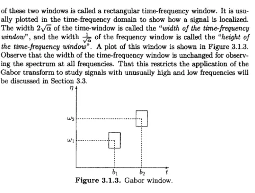
Figure

+4

Documents relatifs