Analysis of bow crushing in ship collision

(1)

ANALYSIS OF

Bow

CRUSHING IN

SHIP COLLISION

by

JI YOUNG KIM

B.S. Naval Architecture & Ocean Engineering Pusan National University , Pusan, Korea, 1996 Submitted to the Department of Ocean Engineering in Partial Fulfillment of the Requirements for the Degree of

MASTER OF SCIENCE IN OCEAN ENGINEERING at the

MASSACHUSETTS INSTITUTE OF TECHNOLOGY

February 2000

Z--)/

Signature of A uthor... ... ... ...

Department of Ocean Engineering January 15, 2000

Certified by... ...

Professor Tomasz Wierzbicki Thesis Supervisor

Accepted by...

MASSACHUSETTSINSTITUTE Professor Nicholas M. Patrikalakis

MASSACHUSETTS INSTITUTE

OF TECHNOLOGY Chairman, Departmental Graduate Committee

(

i --;

(2)

ANALYSIS OF

Bow

CRUSHING IN SHIP COLLISION

by

JI YOUNG KIM

Abstract

Collision of ships with oil tankers poses, next to grounding, one of the most serious environmental threats at sea. In many previous analyses of the collision problem, the bow of the impacting ship was considered rigid. The objective of the present research is to include the finite strength of the bow in the overall collision simulation. The emphasis

will be placed on typical raked shapes because some work already has been reported in

the past on bulbous bows. The main structural members will include side shell and the deck. Transverse and longitudinal stiffeners will be taken into account by means of a smearing technique. A structural model is developed by identifying localized zones of plastic deformations from photographs of damaged ships. Then, the contributions of the membrane and bending resistance is assessed and a simple computational model is developed. The solution includes determination of the force-indentation relationship, a number of folds and a total amount of damage for a given speed of a ship. Five scale model tests were run and the force-deflection characteristics were recorded. A good correlation was obtained between the analytical solution and experimental results.

(3)

Acknowledgments

My appreciation goes to my thesis supervisor, Professor Tomasz Wierzbicki. He gave me great encouragement and support. I also would like to thank Professor Paik who has always been a guiding light of my life, and Professor Mario Maestro and Professor Alberto Marino for providing original of photographs of the DELEDDA damaged bow that initiated the present research.

Finally, I wish to express my deep gratitude to my family for their unconditional love and support through my life. Especially, I would like to say that I am so happy and lucky to have such a great man as my father.

(4)

List of Figure

1 Conceptual Division... 7

2 C ollision O verview ... 8

3 Collision Side View... 9

4 Rankin Field Criterion...11

5 Tresca Field Criterion... 12

6 Von Mises Field Criterion... 13

7 Comparison of the Criteria... 14

8 Typical Plot of Load vs. Axial displacement for Square Box Column...19

9 Deformation Mode... 19

10 Folding Mode A...19

11 Folding Mode B...19

12 One Folding Element... 20

13 Tension Field for Mode A, B...21

14 Minimum Plastic Energy... 23

15 Boundary of the Deformation Part of the Bow ... 25

16 Geometric Parameters...26

17 D eck A ngle... 25

18 D efining Edge Lines...27

19 Diagonal View of damaged DALEDDA ... 29

20 Side View of the damaged DALEDDA ... 30

21 Front View (Model A)...31

(8)

23 Diagonal View (Model A)... 31

24 Close Look (Model A)... 31

25 Front View (Model B)... 32

26 Side View (Model B)... 32

27 Diagonal View (Model B)... 32

28 Kinematics of Deformation Mode (Model A Side View)... 34

29 Kinematics of Deformation Mode (Model A Over View)...35

30 Simplified Stretched Areas (Bow Part)...36

3 1 Flow Stress... 37

32 Membrane Stretching Zone (Bow)... 38

33 Membrane Stretching Zone (Side)...40

34 Folding Element...41

35 D eck B ending... 42

36 Membrane Stretching Zone (Bow)... 46

37 Displacement Function A(y)... 47

38 Nondimensional Wavelength to Thickness... 50

39 Kinematics of Deformation Mode (Model B-Side View)... 52

40 Kinematics of Deformation Mode (Model B-Over View)... 53

41 Membrane Stretching Zone (Side-Side View)... 54

42 Membrane Stretching Zone (Side Si, S2-Over View)... 55

43 Membrane Stretching Zone (Side)...58

44 Kinematics of Deformation Mode (Model B-Method 2)... 62

45 Two Folding Model... 63

46 Folding Measurement... 63

47 Kinematics of two folding case... 65

48 Membrane stretching zones... 64

49 Stiffened bow structure... 69

(9)

51 Equivalent thickness... 69

52 Three folds induce stiffened bow structure...71

53 Kinematics of the three folding bow... 72

54 Strength comparison... 75

55 Strength comparison by fold numbers...76

56 Prediction of the strength increase by fold numbers...77

57 Bow Profile of the Tanker... 80

58 Bow Profile of the Container...80

59 M odel D im ensions... 82

60 Loading Location... 83

61 Fully clamped boundary conditions ... 83

62 Loading C onditions...84

63 Stress-Strain Curve (t=0.71mm)... 85

64 Stress-Strain Curve (t=1.2mm)...86

65 Force-Displacement (Bow-1)... 86

66 B ow 1 Test Picture 1...86

67 Bow 1 Test Picture 2... 86

70 Force-Displacement (Bow-2) ... 87

71 B ow 2 Test Picture I... 87

73 B ow 2 Test Picture 3... 87

75 Force-Displacement (Bow-3) ... 88

(10)

79 Bow 3 Test Picture 4... 88

80 Force-Displacement (Bow-4). ... 89

85 Force-Displacement (Bow 5)...90

87 B ow 5 Test Picture 2... 90

88 B ow 5 Test Picture 3... 90

89 Bow 5 Test Picture 4... 90

90 Force-Displacement (Bow 6)...91

95 Nondimensional comparison of methods... 95

96 Super folding element 1...96

99 Half-length super folding element 1... 98

100 One third-length super-folding element 1...98

101 Two third-length super folding element 1... 98

102 O ne folding elem ent... 102

103 One pair of the super folding elements... 103

(11)

Nomenclature

Stress Flow stress GO

au Ultimate stress

aTy Yielding stress

oGi Stress tensor

71,72, (3 Principal stresses Stress tensor Strain

Strain tensor (Plane stress) Strain tensor

Plastic strain tensor e

U Elastic strain tensor

0 1, 02, 03, 04 0 1 lm lu R1, R2 R3 S

Hinge rotation angle Deck angle

Deformation angle Bow angle

Bow length

Side length ~ Bow length Upper deck length = li Contact point rotation radius

Hinge rotation radius (Model A), Bow tip rotation radius (B) Bow tip rotation radius (A)

Indentation depth Plate thickness

(12)

u U1, U2, U3... A p. H Si, S2, S3... S L B d D V T P Eext Pm Um Us r Ub Em Emi, Em2... Eb Ebi, Eb2... Embo Ems Emst Esf Edb Displacement function Displacement function

Maximum side stretching length Maximum bow stretching length Folding wave length

Stretched areas Surface area

Ship over all length Midship breath Moulded depth Depth

Volume of a body External surface force Instantaneous crush force External work

Mean crushing force Membrane energy Bending energy Membrane energy

Membrane energy of area Si, S2

,.--Bending energy

Bending energy of hinge folding element 1, 2,.. Membrane energy of bow

Membrane energy of side Total membrane energy of side Bending energy of sides

(13)

M

Bending moment

Mo Fully plastic bending moment per unit length

Map Bending moment tensor

N Membrane force

No Fully plastic tension load per unit length Membrane force tensor

(14)

List of Table

1 Predicted mean crushing strength and optimum wavelength 44 (Model A, Method-1)

2 Optimum H (Model A, Method 2) 50

3 Predicted mean crushing forces (Model A, Method 2) 50

4 Optimum spacing length of the transverse stiffeners (Model 57 B, Method 1)

5 Optimum spacing length of the transverse stiffeners 60

6 Dimension by ship type 78

7 Bow length / Plate thickness 81

8 Material properties 85

9 Predicted mean crushing strength (Model B-Method 2) 93 10 Predicted mean crushing strength (Model B, Method 3) 93

11 Predicted mean crushing strength ((Unstiffened two folding 94 model-first fold)

12 Predicted mean crushing strength (Unstiffened two folding 94 model-second fold)

13 Predicted mean crushing strength (Stiffened two folding 94 model)

14 Simplified calculation process 99

15 Calculation of coefficients 103

16 Application to the Bowl, 2, 3, 5 104

17 Calculation of coefficients 105

(15)

Chapter 1

INTRODUCTION

1.1 Background

A ship undergoes wave loads as well as extreme accidental loads in its lifetime. Among many types of ship accident, collision is directly related to the ship structural strength. Especially, collisions of the hazardous substance carriers such as oil tankers, LNG/LPG... can cause serious environment threats when occurring near the coastal areas or narrow channels.

The accident of the Exxon Valdez off the Alaska coast in 1989, and the accident of the Sea Empress in the channel near the Wales in England in 1996, and several other tanker accidents have created serious need for the sea environmental protection and initiated prompt discussions on the methods, which will prevent perilous substance spills such as oil. As a result, the U.S. Oil Pollution Act was introduced in 1990 (OPA 90) that requires double hull tankers in U.S. waters by the year 2015. The International Maritime Organization (IMO) has also established compatible regulation which contains design rules against accidental or extreme loads such as MARPOL 73/78 Annex 13F, 13G.

(16)

A

In preventing environmental disaster the reduction of the human error and the improvement of the traffic system must be first considered. However, it is very difficult to avoid human errors totally. Therefore, it is important to establish rational ship structural design guidelines that minimize the perilous substance outflow of ships. To establish new design guidelines many researchers analyzed mainly two accident scenarios. One is ship grounding and the other is ship collision. Furthermore, the ship collision also can be classified into two groups, side collision and head-on collision. The side collision generally represents a ship-to-ship collision situation. In other words, a striking ship collides with the side structure of the struck ship. A typical head-on collision represents a situation when a bow of a ship collides into a fixed embankment such as pier or bridge crossing international shipping route or gravity-supported offshore installations.

Even though the head-on collision might be treated as a less serious case as compared with grounding case and side collision, there must be no priority in preventing disaster. Moreover, for more than four decades the value of contributions of many design guidelines in this field is questionable. When we evaluate of the progress of the science and technology in late 2 0th, better methods must be developed in this field.

1.2 Current Methodologies

In the history of the ship collision research there have been many methodologies since Minorsky (1959) proposed an energy method for predicting collision damage to protect nuclear power plants. These methods can generally be classified into three categories that are numerical based, empirical based, analytical method.

(17)

The numerical method is mainly based on the commercial finite element computer programs such as DYNA3D, PAM-CRASH, ABAQUS, ADINA, MSC/DYTEAN. This method is becoming popular as computer programs are being sophisticated, and is being widely used especially for a parametric study. However, it needs enormous computing time and efforts in modeling.

The empirical based method was first introduced by Minorsky[2]. He proposed a linear relationship between the resistance and penetration based on statistics of 26 ship-to-ship collision. This method has been widely used by industry, and has been confirmed and modified by many researchers such as Woisin[3 7], Akita[5], Kitamura[3 8],Vaughan[3 9], Hysing,[40], Choi[41],and others.

The analytical method is mainly based on the application of the theory of large plastic deformation of shells. It is appears that Wierzbicki[14] first applied this theory to ship collision analysis with his insightful modeling skill. The paper on the "Intersecting plates method" was published in 1982. Later this theory has been extended and modified by Amdahl[16], Abramowicz[20], Yang,&Caldwell[24], Kierkegaard[29], Paik[33], Pedersen[28].etc. Since this method is deeply rooted in principles of classical mechanics, it is gains increasing popularity and also enjoying high accuracy.

1.3 Previous Research

It is difficult to predict the mean crushing force of the complex bow structure of a ship in a frontal collision. Thus, it was necessary to study simplified bow structure, and many researchers approached the problem through the study of axial crushing of circular cylinders or square tubes. In fact, the mechanism of axial crumpling of thin-walled structures is a common phenomenon in damage of ships' bow during a collision, and it is a crucial element to understand the energy absorption characteristic of structural elements that constitute the bow structure and control its crushing performance.

(18)

-A

An extensive literature surveys by Jones[10] ,van Mater & Giannotti[9] had set up the foundation of the ship collision research.

Nagasawa et al [7] performed structural model tests, simulating the collision of ship side with the buffer placed on the corner part of a bridge pear. They used two kinds of buffer models, referred to as grid-type and composite-type. Through this experiment they compared force-deformation curves of both types of the buffer models and estimated the amount of energy absorbed by the composite-type of buffer in both side and bow collision cases.

Ohnishi et al [15] performed a theoretical calculation by the F.E.M. on an ideal mathematical frame model of bow construction, and compared it with 1/10 scale bow model test results. Through this process they estimated the collapse loads of bow construction of actual ships and obtained the load-deformation curves.

Wierzbicki[14] developed a new method and introduced the term "Crashworthiness". He assumed that a typical ship's hull section consists of an assemblage of plastic plates with "L" "T", "X" shaped "super-folding elements", and calculated mean crushing force of the each elements through equating the rate of the external work and the linear superposition of the bending energy dissipation rate and membrane energy dissipation rate.

Meng et al [17] calculated the mean crushing force of axially loaded square tube using the concept of the moving plastic hinge, and found that the linear relation holds between the folding modes and the ratio of plate thickness per plate width.

Amdahl derived a formula for the mean crushing force of the bow collision with the same assumption as Wierzbicki's and verified it through various types of bow model tests. Abramowicz and Jones [20] develop analytical method to determine the effective crushing distance in axially compressed thin-walled metal columns, and derived an expression for the mean crushing force of the stiffened and unstiffened tube.

(19)

Abramowicz & Jones[23] performed dynamic axial crushing tests on the square tubes which have two different ratios of the plate width to thickness .Through this experiment they checked validity of some assumptions such as asymmetric folding mode, and observed the Euler collapse of the longer columns. They used the effective crushing distance ratio for the calculation of the static mean crushing force, and included dynamic effects by considering the material strain rate sensitivity.

Kawai et al [22] developed the numerical method for estimating the energy absorption of the structural impact in which they modeled structure as a mass spring system based on the Finite Element Method and the axial crushing theory of square tubes due to Wierzbicki, and Abramowicz. In the tests they ignored the inertial force and took the 73% of the initial length as an effective crushing distance, and found good correspondence between the theoretical solution and test results.

Yang & Caldwell [24] proposed a formula based on Wierzbicki's collapse mechanism to predict the mean crushing strength of complex structures and applied to the ship's bow structure collision into a concrete pier. Their formulation included the increment of the crushing strength due to material strain-rate effects and longitudinal stiffeners in the analysis of the energy absorption behavior of panels.

Toi et al [25] performed numerical and experimental study on axially loaded square tube. The experimental data on the buckling load, deformation mode, and mean crushing force were compared the conventional analytical based method, numerical based method, and empirical based method.

Jones & Birch [27] performed experimental study on the axially stiffened square tube. In the experiments the ratio of the column length to plate width was held constant. Studied were effects of the stiffener height, number, inside stiffened case and outside stiffened. They tested both stiffened and unstiffened square tubes under static or dynamic load. In their calculation of the mean crushing force the effective crushing distance were not considered but the dynamic effects were included.

Kierkegaard[29] used an orthotropic theory of plated to take into consideration the effect of stiffeners.

(20)

Pederden et al [28] presented a basis for the estimation of the collision forces between conventional vessels and large volume offshore structures. They derived an expression for the crushing loads as a function of penetrations for different bow structures, and crushing forces as functions of vessels size, vessel speed and bow profile. They also integrated analysis results into the probabilistic procedure for the design of the fixed marine structures against ship collision, based on an accepted maximum annual frequency of severe collision accidents.

Ohtsube and Suzuki [30] improved Yang & Caldwell's technique of deriving simplified equation of mean collapse force, and applied to the ship bow structure. The finite element analysis using MSC/DYTRAN was applied to verify the validity of the approach. The comparisons are made with experiment result of Nagasawa et al [11].

In 1995, Wang Susuki [32] proposed a simple one-term formula for predicting the crushing strength of ship bow structures, through introducing energy absorption ability of structures and energy absorption reduction effect which is caused by inclination load.

(21)

1.4 Motivation

Large ship such as crude oil carrier or container carrier can be considered to be composed of three parts that are bow, mid-parallel, and stem part. In frontal collision usually the damage is confined within the bow part. This is because of a smaller cross-section horizontally and vertically. Furthermore, the bow can also be conceptually divided into two parts that are tetrahedral part Fig. (1) and the remainder. Since the bottom plate does not support the tetrahedral part, it can be considered the most vulnerable part of the ship. In fact, the crushing force and deformation curve of this part of the formulas of the previous researches [16], [24], [28], [32] and tests results show the steep angle increase of the crushing force to indentation depth. Thus, this thesis will focus on the analysis of this tetrahedral part.

TetrahedraPart Tetrahe Part

The rnainder

bottom

Figure 1: Conceptual Division

As far as previous methods for the bow crushing analysis were concerned, they all were derived through a microscopic approach based on Wierzbicki's intersecting plates method using super-folding elements ("L", "T", "X") whether those were improved or expended. Recently, Wang and Suzuki [32] considered the inclination of plate intersection to collision load. However, it is obvious that the reasonable method in mathematics and mechanics to represent an approximate 3-dimensional bow crushing force requires the macroscopic 3- dimensional approach at least for the shell part of the bow.

(22)

Moreover, to develop design guidelines for the ship building industry, solutions must be able to provide an optimum spacing for the stiffeners of the bow structure. Therefore, the author will develop a simple formula that is reasonable both mathematically and mechanically. Through the combination of the kinematic approach due to Wierzbicki's

[14] and the formula obtained for the unstiffened shell part, a one term formula for the mean crushing force is derived, and application to the bow models and the comparison with the theoretical solution is made.

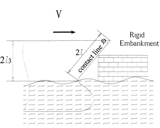
1.5 Problem Formulation

A ship with an orthogonal stiffened bow structure is considered. The ship is moving forward with the initial velocity V and hits the embankment. It is assumed that the contact point of the ship is above the bulbous bow and below the upper deck sideline. The encounting impact angle is 90 degree. vertically and * (bow angle) horizontally. The bow elevation and the trim effect are neglected, thus no friction force between the bow and embankment is considered.

The embankment is assumed to be rigid right angle-edged. The collision is assumed to be perfectly inelastic, thus the external kinetic energy is fully converted to the structural damage of the striking ship.

(23)

V

Rigid

Embankment

21

Figure 3: Collision Side View

The above assumptions simplify the external dynamics of the ship motion. However, the result of the internal mechanics of the collision process to be developed in this report can be used for an overall collision analysis with small modifications.

(24)

Chapter 2 THEORETICAL BACKGROUND

2.1 General

The deformation mode during the collapse of ship's bow structures naturally involves very large strains, and strain rates well into the plastic range. The material behavior after yielding is nonlinear and elastic effects are negligible. Therefore the behavior of structures can be treated as rigid-plastic. The Following three sections provide review of the elementary theory of plasticity.

2.2 Yield Criteria

For a one-dimensional body under a one-dimensional stress state, it is relatively simple to define and find experimentally the yielding point. Plasticity occurs when the stresses attain a certain material-dependant value termed the yielding stress. However for more than one-dimensional bodies under combination of stresses, the situation is not so straightforward and several theories were advanced to define yielding criteria that help us to find a direct comparison with simple uniaxial yield stress of the tension test. The most important three yielding criteria are the criterion of Rankin, the criterion of Coulomb-Tresca, and, von Misses yielding criterion.

(25)

A. Criterion of Maximum Principal Stresses of Rankin and the Deviator Tensor

This criterion, for which good agreement with experiments on brittle material was found, assumes that yielding limit of the material is defined by the simple uniaxial test. For a two-dimensional stress state, this can be represented by the quadratic yielding boundary sketched in Fig.4. This simple yielding criterion encounter difficulties related to experimental observation such as hydrostatic pressure that has no effect on yielding. The experimental fact implies mathematically that yielding is not affected by the first invariant of the stress tensor, I=

ax+oy+az =a I +a2+3 ,as shown in the following analysis.

Thus a- = o-,, o-, o (1)

can be regarded as the result of the superposition of two stress

ax -P Ua, ax P

a= [o-, - -P og + P (2)

U.,, Ue, a -P_ P_

where P is the hydrostatic pressure

1 1 1

p =-(o + Y+o- + )= -(o- 1 + 2 +o)= -I (3)

3 3 3

G 2

(26)

The tensor notation is:

7-, =a,+pI (4)

where, I is the unit spherical tensor and aij is the stress deviator tensor simply referred to as the deviator, and yielding depends of the deviator only.

B. Coulom-Tresca Criterion of Maximum Shearing Stresses There is also an experimental observation which may agree with the intuitive expectation that yielding in the case of a two-dimensional tension-compression stress state will occur earlier than for tension-tension or compression-compression. In this way, another criterion due to Coulomb and Tresca can be viewed. Mathematically, Coulomb-Tresca yielding can be stated as follows:

[(os -a~2) -U )[(0~2 -0a)2 _.)[ )2 -o )]= 0 (5)

The plasticity boundaries given by this criterion are shown in Fig 5. for the two-dimensional stress state.

G3

CYyI

Figure 5: Tresca Field Criterion

When (GI, u2=G3=0), one obtains a1=a y. As expected, it is reduced to the known one-dimensional stress state yielding. When a1=-03, C2=0, one obtains ai=±1/2a

(27)

C. von Mises Criterion

A yielding criterion developed by Beltrami, Huber, von Mises and Hencky, and which stood better with experimental results, especially for ductile material, is that of maximum distortion energy which is frequently referred to as the von Mises yielding criterion. Mathematically, this leads to the condition.

(o- a2) +(o - +(o -0a) 2 = 2-, (6) In two-dimensional stress space, this condition forms an ellipse such as that shown in Fig.6. When a2=a3=0,one obtains ai=ay while in the case of

11

S=

±

Ia, as compared to o = ± -o-, in the previous case of the

Coulomb-73 2

Tresca yielding condition. In Fig. 7 all these conditions are compared together and it be seen that they are identical for four points only and that the difference between the condition of Tresca and von Mises is minor.

G3

>/ I

Figure 6: von Mises Field Criterion

The Tresca criterion is often applied to derive analytical solution of elastic-plastic problems, due to its simple linear form. The von Mises criterion has a nonlinear form in terms of stress components, and is therefore more complicated to use. Various plasticity theories exist. For strain hardening materials, the most common are the deformation

(28)

theory and the incremental theory. The deformation theory totally neglects the loading history dependency, and is therefore the simplest and the one most extensively used in engineering practice. The incremental theory does consider loading path dependency, and

is thus somewhat more complex.

When the material is idealized as perfectly plastic the analysis is greatly simplified. For such materials, the limit theorems of plasticity may be established. These theorems can be used to develop methods for estimation of load-carrying capacity of structures. Perfectly plastic materials may be described by the flow theory, which is presented in next section.

von Mises

ellisp

G3

$

ay

(29)

2.3 The Flow Theory of Plasticity

The yielding function is considered to remain constant as plastic deformation progress for a perfectly plastic material. Thus the yielding condition can be expressed as:

f(o-1) = 0 (7)

The total strain increment tensor can be assumed as the combination of the elastic and plastic parts:

dc =de' + ds (8)

The ratio of the components of the plastic increment tensor de that defines the direction of the plastic strain increment vector de in the space, and is called flow rule can be expressed as:

de? =dA (9)

where dA is a positive scalar factor of proportionality that is nonzero only when plastic deformation occurs.

The combination of the flow rule and yielding criteria will give us the components of the plastic strain increment. The very general properties of the yielding material are the Druckers' stability postulate, which considers that a material body subjected to certain surface and body forces, including certain displacements, strain, and stresses. He postulated that stable system that satisfies equilibrium and compatibility conditions is one that satisfies the following conditions

A. When an additional set of forces are applied, the work done by the additional forces and the associated changes in displacement are positive.

S> 0 (10)

B. Over a cycle of adding and removing an additional set of forces, the work done by the additional forces and the associated changes in displacements are non-negative

Both conditions imply that the yield surface must be convex, and the plastic increment vector must be normal.

(30)

2.4 Limit Analysis

Development of an estimation method for the collapse load of a structure requires an idealized body. Two basic assumptions are made for such a body.

A. Perfectly plastic material: The material shows perfect plasticity character with the associate flow rule without strain hardening or softening

B. Small structural deformations: Changes in geometry of the body or structure that occur at the limit load are negligible hence, the geometric description of the body or structure remains unchanged during the deformation at the limit load. The second assumption allow for the use of the virtual work principle:

JT,Su, dS+ JF,8u, dV = f-,Se dV (12)

S V

where Ti are surface forces and Fi are body forces, and ,a is a set of stress state in equilibrium with Ti and Fi while &Y is a set of strain increments compatible with the displacement increments u,. The left hand side represents external work increment 8Ee, on the body, and the right hand side represents internal work increment gEint dissipated in the body.

For the above equation, any equilibrium set may be substituted into. For example, the rate

of change of displacements and strains(tu, ) can be used, and expressed as follows:

JTiidS + f Fj *1i dV f=a, dV (13)

SVV

Generally, there are three basic relations that must be satisfied for a solution of a problem in solid mechanics. These are the equilibrium equations, the constitutive relations, and the compatibility equations. In the limit analysis, a lower-bound solution is found by only considering the equilibrium equations and constitutive relations, and an upper-bound

(31)

C.

Lower Bound Theorem: If an equilibrium distribution of stress o can be found which balances the body force F in the volume V and the applied load T,

on the stress boundary Sr and is everywhere below yield f(o) <0 then the body at the loads T, F will not collapse.

D. Upper-Bound Theorem: If a compatible mechanism of plastic deformation

O.P *P

ei;,u,; is assumed which satisfies the condition ui, =0 on the displacement

boundaryS, then the load T, F, determined by equation energy dissipation will be either higher than or equal to the actual limit load.

When applying the upper-bound theorem, a kinematically admissible displacement field is used to equate the rate of work done by external forces of the internal energy or rate of energy dissipation. In practice application, the collapse mode can often be predicted from geometrical consideration. Kinematically admissible displacement fields can then be found, and the upper bound theorem is therefore particular useful.

(32)

Chapter 3 REVIEW OF THE THEORY

3.1 Crushing Strength of Plate Intersection

A typical cut through a ship's hull consists of an assemblage of plates with various shapes of stiffeners. However, one can distinguish three structural configurations, that is Angle elements "L" (Two intersecting plates), "T" elements (Three intersecting plates), "X" elements (Four intersecting plate). The crushing strength of plate intersection can be represented by the mean crushing strength of these elements that can be calculated through the energy absorption of the super folding elements. As a simple example of the method, the calculation of the mean crushing force of the thin square tube is considered.

A. Mean Crushing Strength of a Square Tube

The analysis of the crushing mechanism of the thin plate structure provides a solution for the relation between the load and displacement. But it is very difficult to find the instantaneous force, and it is more convenient to calculate the mean crushing force as shown in Fig.8, which means that if we know the mean crushing force, we can find the corresponding amount of the absorbed energy for a given crushing distance.

(33)

ultimate strength Pu

mean crushing strength

end of loading Pm

rigid behavior crushing behavior

Indentation 6

Figure 8: A Typical Plot of Load vs. Axial displacement for Square Box Column

B. Simplified Deformation Mode

There can be many deformation modes, and if the ratio b/t is very large, typically over 100 often collapses in asymmetric, irregular deformation modes, and the incompatibility of folding modes is of frequent occurrence. Shown in the figure below are two typical symmetric A and B, and the calculation is based on mode A.

Figure 9:Deformation Mode

H Folding Mode A Figure 10 Folding Mode B Figure 11 I

(34)

--ZZT--The known parameters are width b, thickness t, flow stress ao, and the unknown parameters are crushing strength P, half folding wave H.

C. Principle of Virtual Velocity

The crushing strength can be found through the Principle of Virtual Velocity.

PS -= &+&M (14)

The left hand side represent rate of external work, and the left hand side represents a sum of the rate of the bending energy dissipation and membrane energy dissipation.

P

H H

Figurel2: One Folding Element

From the geometry of a single fold: 5 = 2H(1 - cos a)

S = 2Hsinaa

5max =2H

The integral form of the principle of virtual work is.

P -dt = 0 fP - d P-dt = 0 1"'" 0 bdt+ U,, dt 0 P(S)dS = { P(S)dS}SPma , ,-2H max 0

Ub : rate of bending energy

Um :rate of membrane energy (15)

(35)

Mean Crushing Force is defined as: ,5max P, =n {TP(c)d9} 5max ₀ And I= Ub = Jadt (17) 1I Um = JU,,dt 0

3.2 Membrane Resistance

The rate of membrane energy dissipation can be expressed as follows:

Un = N,, a, dS (18)

S

The assumption for the strain tensor, and the fully plastic membrane force tensor are:

0 0 0 0 (19) = N ₀ 0 0

An approximation of the total membrane stretching energy can be obtained by considering only final stage of deformation. The velocity rate of the strain follows:

'd u

e

d= (20)

dx

From the deformed model A, the displacement field can be found as linear function of y:

u(y) = Y H = y (21)

H

all 0 u(y)

HJY

(36)

Substituting equations (19), (20) into (17), the equation becomes A' H b U = 2f N 0 0 du H dx dxy = 2JfNou(y)dy 0

u(y) =u(x = b, y) - u(y = 0, y) Therefore, the membrane energy for the model A becomes:

H

Urn = 2N₀ fu(y)dy = NoH 2 0

For the alternative model B, the membrane energy becomes:

Ur =No H 2

H where H becomes H 2 Normalization with respect to M.

energy of one plate intersection:

002

= -tgives the 4

Ur =Mo

t

final expression for the membrane

(25)

3.3 Bending Resistance

The rate of bending energy dissipation can be expressed as follows:

n

U, = MoOi b, =4MO

Ob

i=0

Therefore, the bending energy for the model B becomes: ;r

2

Ub = JUbdt= 4Mob dO = [Mob0] = 21rMob

0 0 where (22) (23 (24) (26) (27)

(37)

3.4 Global Equilibrium

Energy balance equation for the one complete folding that does not involve the current indentation depth, 6: P,,, -2H = U, +Ub H 2 P, -2H = 2MO -+2;r Mob (28) t P H b Mo t H

It is postulated that H adjust itself so as to minimize the mean indentation force. Which means that the length of the folding wave Hopt is still to be determined, and it can be found by minimization of Pm with respect the H.

PM1 Bending Contribution Membrane Contribution O Hopt H

Figure 14: Minimum Plastic Energy dP.

dH

-z b = 0 ₍₂₉₎

t H 2

=>Ho, = bt

Eliminating the wavelength H from the equation (27), the final expression for the mean crushing force per one contributing flange becomes.

Pb 2 i

-Mo

t ₍₃₀₎ P = 2 -ot b 20 A

(38)

Chapter 4

SIMPLIFIED MODEL

4.1 Simplified Geometry

Since the bow has a complex three-dimensional shape, it is necessary to simplify the bow geometry. As already mentioned in Chapter 1, this thesis deals with the tetrahedral part that is most vulnerable part of the bow structure. In this thesis the tetrahedral part will be called just "bow" for convenience.

A. Boundary of the Deforming Part

The first step is to specify the contact point between the ship and the rigid obstacle, and defining the tetrahedral part on the bow structure. From the observation of the actual accidents and model tests it was determined that the contact point divides the bow length in two parts with same length, and the vertical extension of the line from the end of the bow length to the deck plate defines the extent of the deforming part of the tetrahedral part of bow structure Fig 1, Fig 15.

B. Bow Parameters

The second step is to define the bow model with simple geometric variables keeping the number of variables as few as possible. In this thesis the simplified

(39)

model involving three input parameters, which are the bow length (1), bow angle (p), deck angle (0). The bow length is twice of the length between the apex and the contact point. The bow angle, as shown in Figure 15, is the angle between the upper deck and contact line. The deck angle shown in Figure 16 is the approximate angle taken in the upper deck horizontally and between the forefront and 15 vertically.

C. Defining the lines

The third step is to define all the edge lines in terms of the given parameters (1, p, 0). By this step the approximate computation procedure of the internal energy dissipation including all the edge lines will be simple and the final formula for the mean crushing force will be compact. Fig 15.

A.

(40)

I

Figure 16:Geometric Parameters

(41)

L

3

Figure 18: Defining Edge Lines

The length of the edge lines in Figure 3.4 can be expressed as:

l =2lcosqp

/2

2 1 Cos (

cos 0

13 =lsinq(

/4 =lcosp (31) 15 = 4l cos

ptan0

(42)

Chapter

5

SIMPLIFIED DEFORMATION MODEL

5.1 General Considerations

In constructing a deformation model it is important to keep the folding mode simple, and still reproducing the real deformation shape. In search for the kinematically admissible displacement fields, photos and various paper models were used. In this crushing scenario it is assumed that the velocity of the ship is constant for the entire crushing process. Alternatively, it can be also assumed that the bow part is fixed with suitable boundary conditions and the embankment crushes the bow with a constant velocity V. Since the indentation displacement changes from zero to 6i the mean crushing force Pm over the range (0 6 61) can be defined as:

I'

=i

f'P(85)dd ₃₂

where P(6) is the instantaneous crushing force So, the total work of the external forces becomes:

E, = P(5)d5 = P,,-. (33)

Three bow models were developed. Historically, the model with outward folding (Model A) was developed first. However, the crushing force predicted by the corresponding

(43)

models (Model A and Model B) were created with inward folds that gave satisfactory results. The 'outward' model calculation is performed in section 6.1, 6.2 and the inward folding models for the first folding were calculated in section 6.3, 6.4. Since the inward first folding model gave us a satisfactory result, this model B was used for the calculation of the second folding case and transversely stiffened case in section 6.5, 6. 6.

5.2 Real Ship Collision

Photographs of the real accident observed show quite a complex deformation mode, Fig.18. However, by careful inspection, it is observed that there are four major internal energy dissipation areas, which are side shell folding, deck tilting, frontal bow stretching, and side shell stretching. It is also noticed that one fold of the side shell of the bow matches one bent on the deck and the large stretching area from the contact point and

small stretching area on the sides.

Figure 19: Diagonal View of damaged DALEDDA (Courtesy of M..Maestro and A. Marino)

(44)

-o

rJ)

(45)

5.3 Three Dimensional Paper Model

Figures (20-26) show the paper models used in computation. Shown in these photos are simplified membrane and bending zones. The displacement field was defined in terms of the simple geometric parameters defined in the previous section.

Model A

Figure 21: Front view (Model A) Figure 22: Side view (Model A)

(46)

Model B

Figure 25: Front view ()

gure 26: Side view (Model B)

(47)

Chapter 6 STRENGTH OF THE BOW STRUCTURE

6.1 Mean Crushing Strength (Model A)

The calculation of the mean crushing strength of the deformation model A that folds outwardly is constructed, and two computational methods are tried in the subsection I and 2. The first method is based on the final deformation shape and the second is based on the deformation paths.

1. Method-1

A. Kinematics of Deformation Mode A

While the embankment moves horizontally along the 16 the initial contact point

is divided in two part, as shown in Figure (28, 29), and moves along the RI and R2 with radii I and 13. When the indentation depth becomes 6, the vertically overlapped distance of the initial contact point is denoted as t, the other point

Q

follows similar procedure, and stretches out with distance A. Consequently, the stretched zones Si, S2, S3, S4, S5, and S6 are formed and the side shell is folded.

This procedure can be restated that the upper bow part and lower bow part divided by middle horizontal cross section rotate by the angle P, and the side shell is folded with wavelength 2H. For simplicity, the above lengths are expressed in terms of I,

p,

p as follows:

p = 2/{sin(9 + ,8) - sin y}

A = 21sin qp( - cosfp) ₍₃₄₎

H =-6 sin

2

Thus, the angle P and the length of the folding wave 2H uniquely define the geometry of the fold.

(48)

L1

(49)

(50)

B. Frontal Bow Stretching

The areas SI, S2, S3, and S4 that are made up of two triangular shaped cross-sections visualizing deformation zones of frontal bow stretching. Those stretching areas are developed from the contact point where the contact line and the rigid-embankment meet. As the embankment penetrates deeper, the angle 2p in between two horizontal cross sections will be increased. However, the areas will grow only to a certain angle of

P.

When the initial contact points rotate up to

p,

the indentation depth 5 becomes 2H.

x

Z S2

$422P

Figure 30: Simplified stretched areas (Bow part)

Assumption is made that for the strain is uniaxial in the local coordinate system

0 0

0 (35)

Rigid perfectly plastic isotropic material is assumed: 0 0

N - 0 N ₍₃₆₎

where No = -ot is the fully plastic membrane force per unit length and o-o is the average flow stress of the material, see Figure 31.

(51)

M11

GTo

M0

Figure 31: Flow Stress

With the above assumptions the membrane energy dissipation becomes:

E, = s N ,pdS = J No e,,,dS (37)

As shown in Figure 32, in this deformation zones the strain rate is uniform in x direction and varies in y direction, thus the displacement function Ui and U2 for

the stretching zones (0 la) and (0 ! 17) are found as: u1A

2 18

(38) U 2 =

217

In performing integration over the deformation zones S1, S2, S3, and S4, a local coordinate system (71, 4) is introduced. Therefore, the strain &s, over the deforming zones is a function of a and 4:

dU, dU₂

(52)

Figure 32:Membrane Stretching Zone (Bow)

The membrane energy dissipation for total deformation zones by the above expression can be expressed as:

SdU

EM = 2f NO d dqd = NS, = -- cot/p

00 d7 4

As shown in Figure 32 the deformation zones SI, S2, and S3, S4 are identical,

therefore the total membrane energy of the frontal bow stretching becomes:

Embo= EmI + Em2 +Em3 +Em4 =2Emi +2Em2

= 2Nl12 cot/p{sin(cp +p) - sin } 2 (41)

+2NO1 2 _{cot/p sin}2

p(1 - cos/p)2

Since the angle

p

is assumed small, the above expression can be written as:

Embo =2NOl2_/fcos2

(p (42)

(53)

C. Side Shell Stretching

The areas S5 and S6 that are the areas found between two folding elements

simplify the deformation zone of the side shell stretching. In this deformation model the side shell folding is idealized in the triangular and rectangular shapes and fold is formed as the l rotates in clockwise. Since the length Is rotates, there must be a stretched area to meet the difference of the length. As shown in

Figure 32 the stretched length U can be expressed as:

UX =A - A

2H (43)

2

The membrane energy dissipation of the one side can be expressed as follow:

EMS = E ₅+E ₆

=NO(S 5 +S6)

(44)

=No( 3s+S

2

where E5 and E6 are:

E,5 = No C,,,,dS = 2 fNos,₀₁ d7 d S 0 0 2 NOUod't= NoS5 0 2Hq E.6 = Noerr7dS = 2

f

JNOerd d"': S H 0 ₍₄₅₎ 2 H 2 NOU0dg= NOS6 H

Therefore, the side stretching in both sides becomes as:

E,,st = 2Ems

= 3NOAH (46)

(54)

x

S6~ H

S5___

H

Figure 33:Membrane Stretching Zone (Side)

D. Side Shell Folding

The rate of the bending energy of the side shell folding is calculated from the folding element. In this model (Model A) four identical folding elements are deformed at the same time by the external load. A folding element has four stationary hinge lines, and the bending energy dissipation is calculated from the rotation of these hinge lines. As soon as the as external force is applied the side shell is being folded with wavelength H until another folding is formed. The rate of bending energy of the one folding can be calculated as a sum of the contribution from the four straight hinge lines:

4

EbI = MOi 13i (47)

In the above expression it is also assumed that the fully plastic bending moment develops is defined by:

MO = a* t2 (48)

(55)

/COS H Y

'H

Y 12H

z

Pmn X

Figure 34: Folding element

As shown in Figure 34 the length of the each hinge line is different. However, if the angle

P

is assumed small, all hinge lines can be treated as having the same length 1. With the above assumption the expression for the bending energy can be written as:

4

E = fEbidt =4Mo l3 ' dt (49)

i=1

0 0 (49

where 9 is the rotation rate of the plastic hinge, and the 9 293, and 94 are assumed same. The ti is the total time for the whole deformation process when the 0 reaches 0_max._{Therefore, the above expression can be expressed as:}

Eb = 4M 1o d" d. dt b103J 0 46H --5 2 -[-g 2 H = 4MO 13 cos-I (1 - )1 2 (50) 12H -0 = 2;rMO 13 sin (p

Since the four folding elements are deforming at the same time, the total energy dissipation of the side shell folding is:

(56)

E. Deck Bending

As shown in Figure 35 the rigid body motion of the upper frontal part of the bow is supposed to bend the deck plate. If the thickness of the deck plating is the same as the thickness of the side shell, the expression of the deck bending energy dissipation can be written as:

=db M=

Nis

(52)

Edb = Ebbdt _=Mo1₅f /dt

= 4MO1/cos ptan0

= 4MOS cos(ptan0

When the indentation depth 6 reaches 2H, the above expression becomes:

Edb = 8MO H cos p tan9 ₍₅₃₎

/

(57)

F. Global Equilibrium

With the calculated membrane energy and bending dissipation the crushing force can be found from the global equilibrium. The total external work is:

Eet, = P,,, -2H (54)

where Pm is the mean crushing force. The integrated form of the principle of the virtual work is:

P,2H(E, Eb)cosO (55)

Using equations (41), (51), (53) and (55), the mean crushing force becomes:

P-l/, sin p =(E,.b, + E,,,, + E + Edb ) cos0

(56)

= (2No 12_{/ cos}2 ₊_{8xMol sin 9 + 4M}

01l cos y tan O)cos O

P,, (2Nolcot p cos p + 8MO -+ 4M cotytan0)cos0 (57)

It is postulated that the wavelength H adjusts itself to minimize the mean crushing force. In order to find the unknown H, the mean crushing force is minimized with respect to H (l,1p)

dP,,, _-=, P,,, 8l _- _-,_{l+ ap}8Pm, 8/3- _{1 = 0} (8

(58)

dH al 8H 83 8H

We can find optimum H:

H,, =-t tan " 9 (59)

2

Substituting the equation (59) into (57), we can obtain the expression for the mean crushing force:

(58)

Following table shows the equation (59), (60)

optimum H and Mean Crushing Force (Pm) predicted by the

Table 1: Predicted Mean Crushing Strength and Optimum Wave Length p 0 L(rnm) t(mm) cro(Mpa) Hopt(mm) Pm(N) Bowl 60 30" 130 0.7 312 3.297 56828 Bow2 60" 300 65 0.7 312 3.297 28436

Bow3 600 300 87 0.7 312 3.297 38045

Analysis of bow crushing in ship collision

ANALYSIS OF

Bow

CRUSHING IN

SHIP COLLISION

Z--)/

(

ANALYSIS OF

Bow

CRUSHING IN SHIP COLLISION

Abstract

Acknowledgments

Contents

List of Figure

Nomenclature

M

List of Table

Chapter 1

INTRODUCTION

1.1

Background

1.2

Current Methodologies

1.3

Previous Research

1.4 Motivation

1.5 Problem Formulation

V

Rigid

Embankment

21

Chapter 2

THEORETICAL BACKGROUND

2.1

General

2.2

Yield Criteria

CYyI

C. von Mises Criterion

±

von Mises

ellisp

$

2.3 The Flow Theory of Plasticity

2.4 Limit Analysis

C.

Chapter 3

REVIEW OF THE THEORY

3.1 Crushing Strength of Plate Intersection

3.2 Membrane Resistance

3.3 Bending Resistance

Ob

3.4 Global Equilibrium

-Mo

Chapter 4

SIMPLIFIED MODEL

4.1 Simplified Geometry

A. Boundary of the Deforming Part

B. Bow Parameters

C. Defining the lines

L

/2

cos 0

13 =lsinq(

ptan0

Chapter

5

SIMPLIFIED DEFORMATION MODEL

5.1 General Considerations

=i

5.2

Real Ship Collision

5.3

Three Dimensional Paper Model

Model B

Chapter 6

STRENGTH OF THE BOW STRUCTURE

6.1 Mean Crushing Strength (Model A)

1. Method-1

Q