HAL Id: hal-01838371
https://hal-amu.archives-ouvertes.fr/hal-01838371
Submitted on 5 Oct 2018HAL is a multi-disciplinary open access archive for the deposit and dissemination of sci-entific research documents, whether they are pub-lished or not. The documents may come from teaching and research institutions in France or abroad, or from public or private research centers.
L’archive ouverte pluridisciplinaire HAL, est destinée au dépôt et à la diffusion de documents scientifiques de niveau recherche, publiés ou non, émanant des établissements d’enseignement et de recherche français ou étrangers, des laboratoires publics ou privés.
High-Speed Force Spectroscopy for Single Protein
Unfolding
Fidan Sumbul, Arin Marchesi, Hirohide Takahashi, Simon Scheuring, Felix
Rico
To cite this version:
Fidan Sumbul, Arin Marchesi, Hirohide Takahashi, Simon Scheuring, Felix Rico. High-Speed Force Spectroscopy for Single Protein Unfolding. Methods in Molecular Biology, Humana Press/Springer Imprint, 2018, pp.243-264. �10.1007/978-1-4939-8591-3_15�. �hal-01838371�
High-speed force spectroscopy for single protein unfolding
Fidan Sumbul1, Arin Marchesi1, Hirohide Takahashi2, Simon Scheuring2, Felix Rico1*
1U1006 INSERM, Aix-Marseille Université, Parc Scientifique et Technologique de Luminy, 163
avenue de Luminy, 13009 Marseille, France.
2Departments of Anesthesiology, Physiology and Biophysics, and Biochemistry, Weill Cornell Medical
College, 1300 York Ave, New York, New York 10065, USA
Correspondence:
Abstract
Single molecule force spectroscopy (SMFS) measurements allow quantification of the molecular forces required to unfold individual protein domains. Atomic force microscopy (AFM) is one of the long-established techniques for force spectroscopy (FS). Although, FS at conventional AFM pulling rates provides valuable information on protein unfolding, in order to get a more complete picture of the mechanism, explore new regimes and combine and compare experiments with simulations we need higher pulling rates and µs-time resolution, now accessible via high-speed force spectroscopy (HS-FS). In this chapter, we provide a step-by-step protocol of HS-FS including sample preparation,
measurements and analysis of the acquired data using HS-AFM with an illustrative example on unfolding of a well-studied concatamer made of 8 repeats of the titin I91 domain.
Keywords: high-speed force spectroscopy, atomic force microscopy, protein unfolding, titin, dockerin,
cohesion
1 Introduction
As the last step of the central dogma in molecular biology, understanding protein folding is still a fundamental challenge in biology, but also from a physical point of view [1-3]. The folding of
proteins into their native conformations to perform function is one of the most essential processes within the living cell, as proteins are responsible of many biological processes in living organisms, such as catalysis of metabolic processes, gene expression, transport of molecules/solutes between and across the cell, cellular communication and molecular recognition. The unfolding of proteins by mechanical force is also biologically relevant as, many proteins, such muscle protein titin in muscle cells, spectrin in red blood cells and the integrin/cytoskeleton linker talin, are subjected to mechanical
cues and often unfold to function [4-8]. Force spectroscopy (FS) using nanotools, such as magnetic tweezers, optical tweezers and AFM, allows the manipulation of individual proteins and monitoring of the forces required to unfold individual protein domains or subdomains [9-14]. This method provides information about the mechanisms of folding and unfolding under an applied force, allowing the characterization of the (un)folding energy landscape along the axis of applied force.
FS using AFM is a well-established technique, however, the time resolution is limited to a few hundred of µs [15]. The recent development of high speed AFM (HS-AFM) using micrometer sized cantilevers [16,17] and its application for force measurements (what we name high-speed force spectroscopy, HS-FS) provides access to the µs timescale and mm/s pulling velocities thanks to their low viscous drag coefficient [18-21]. HS-AFM cantilevers, with common dimensions of about 8µmx2µmx0.1µm, are considerable smaller than conventional AFM cantilevers. These reduced dimensions give access to the velocities of all atom molecular dynamics (MD) simulations and allow, thus, direct comparison of unfolding forces. Force spectroscopy using HS-AFM cantilevers allowed revisiting well-studied protein systems with better force and time resolution, revealing unfolding intermediate states and accessing new dynamic regimes predicted by theory [22,23].
The use of micrometer-sized cantilevers for force spectroscopy measurements is emerging and, thus, still presents important bottlenecks. The optical lever detection method involves the focalization of the laser into a spot of a few µm wide cantilever, which leads to substantial optical interference artifacts [19,24]. This effect is particularly important when using highly reflective samples, like gold-coated surfaces, a common practice for AFM unfolding measurements using cysteine residues to immobilize the proteins [25,11,5]. Although tilting the sample support by 45º and using low coherence sources, such as superluminescent diodes [18], can minimize optical interference, it still represents a major issue to be solved in AFM in general, and in HS-AFM in particular. Apart from potential optical
geometries. Indeed, conventional AFM cantilevers with blunt tips, which provide a larger contact area between the tip and the sample, frequently used for force spectroscopy as they enhance the probability of picking up molecules, are commercially available. This is not the case for HS-AFM cantilevers, which feature sharp tips appropriate for imaging. While nickel sputtering has been used in the past to enlarge the tip radius and favor binding with histidine tags, the resulting binding probability remained extremely low, of ~1 per 1000 or less. Finally, in some HS-AFM setups [16] [26], the small
piezoelectric elements that allow high pulling rates limit considerably the size of the sample support, limiting the type of surface used to immobilize the protein. Thus, more robust techniques for protein immobilization are important to improve binding efficiency and reproducibility in HS-FS
measurements. The recent discovery of mechanically ultrastable receptor/ligand complexes now allows protein unfolding experiments by grabbing the molecule from specific sites, with precise knowledge of the pulling direction and with higher efficiency than previous methods based on unspecific attachment. [27-31] One of the most versatile methods uses the ultrastable complex formed by dockerin/cohesin III. In practice, a DNA construct is engineered concatenating the protein to be studied and dockerin III. This construct is covalently immobilized to the sample with the free end exposing dockerin III to the bulk, while cohesin III is covalently attached to the tip [32,29]. The dockerin/cohesin III complex dissociates at forces above 300 pN at conventional pulling rates which is higher than the unfolding forces of most proteins, it also provides an unfolding fingerprint that further allows identification of specific unfolding events. This assures specificity of unfolding of the desired protein, proper
orientation, reversibility and reproducibility, while avoiding the use of highly reflecting surfaces, such as gold. Therefore, using this ultrastable molecular complex turns out to be an excellent option for HS-FS measurements.
In this chapter, we describe the use of HS-FS unfolding measurements on single molecules, addressing the specificities of using small cantilevers and sample supports and the construction of chimera proteins featuring the dockerin III domain and their covalent immobilization on the tip and
sample support. Although the chapter is written having in mind the Ando-type HS-AFM
(commercialized by RIBM, Japan), the adaptation to other AFM systems is straightforward and we provide some notes in that sense.
2 Materials
2.1 Protein expression and purification
1. BL21(DE3) competent E. Coli cells.
2. LB-Agar solution prepared according to the provided instructions with kanamycin monosulfate (50 µg/mL).
3. LB-Broth solution prepared according to the provided instructions with kanamycin monosulfate (50 µg/mL).
4. 2 mM CaCl2 solution.
5. Lysis Buffer: 100 mM NaCl, 20 mM Hepes-NaOH, pH 7.6, 2 mM CaCl2.
6. PMSF (phenylmethylsulfonyl fluoride) stock solution: Prepare a 0.1 M stock solution of PMSF (MW 174.2) in isopropanol. Aliquot and store at -20°C. Note that the half-life is short in aqueous solutions (110 min at pH=7 and 35 min at pH=8).
7. IPTG (Isopropyl β-D-1-thiogalactopyranoside). 8. DNase I, Triton X-100.
9. Imidiazole stock solution: Prepare a 5M imidiazole (MW 68.1) stock solution and adjust the pH to 7.6 with HCl. Store at -20 °C and protect from light.
10. Wash Buffer: 100 mM NaCl, 20 mM Hepes-NaOH, pH 7.6, 50 mM imidiazole, 2 mM CaCl2 (see Notes 1-2).
imidiazole.
12. Dialisys Buffer: 100 mM NaCl, 20 mM Hepes-NaOH, pH 7.6, 2 mM CaCl2.
13. Ni-NTA affinity resin.
14. Dialysis membranes with a 10K molecular weight-cutoff (MWCO). 15. Orbital shaker incubator to grow bacteria.
16. OD600 (optical density at a wavelength of 600 nm) spectrophotometer to measure bacterial
growth.
17. Centrifuge and appropriate rotors to harvest bacteria and pellet the bacterial lysate.
2.2 Surface functionalization 2.2.1 Equipment
1. Silicon nitride cantilevers (AC10DS, Olympus).
2. 1.5 mm diameter glass surface (glass rods or cover slips). 3. Ozone or plasma cleaner for cleaning cantilevers
4. Oven to bake cantilevers and glass surfaces
5. Fine stainless steeltweezers for handling cantilevers
6. Pyrex Petri dishes/similar inert vessel for treating cantileverswith acetone, acids, and other reactive reagents.
7. 24-well tissue culture plate for rinsing and treating cantilevers 8. Parafilm
2.2.2 Chemicals
1. Nanopure MilliQ water.
2. Phosphate Buffered Saline (PBS): 10mM Na2HPO4, 1.76mM KH2PO4, 137mM NaCl,
2.7mM KCl pH:9 and pH:7.2
3. HPLC grade or >95% purity acetone.
4. Analytical grade or >99.9% purity ethanol (EtOH).
5. Piranha solution (75% sulfuric acid (H2SO4) and 25% hydrogen peroxide (H2O2)
6. 5% (3-aminopropyl)-dimethyl-ethoxysilane (3-APDMES) in EtOH 7. 5mM Maleimidopropionyl-PEG(27)-NHS Ester in PBS pH:7.2
8. 20 mM Coenzyme A trilithium salt (93%) in 50 mM Na2PO4, 50 mM NaCl 10 mM EDTA
pH 7.2.
9. 1 µM Sfp phosphopantetheinyl transferase in 50 mM Hepes-NaOH, pH 7.5. 10. O2, Argon and N2 gas
2.3 High-Speed Atomic Force Microscopy (HS-AFM)
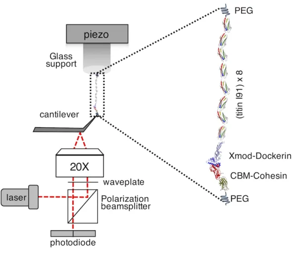
1. Ando-type HS-AFM (SS-NEX HS-AFM, commercialized by RIBM, Japan). HS-AFM has some particularities: small piezoelectric elements, an optical microscope objective to focus the laser into a µm-sized spot and fast acquisition boards (see Note 3) (Figure 1).
[Place Figure 1 here].
2. Micrometre sized AFM cantilevers (see Note 4, Figure 2) [Place Figure 2 here].
3 Methods
3.1 Protein Purification and Sample Preparation
As a well-studied system in the literature, here we use a concatamer made of 8 repeats of titin I91 domain with a dockerin III complex covalently immobilized on the sample support via ybbR peptide (DSLEFIASKLA) as an exemplary system to describe unfolding measurements with HS-FS. The 8 concatenated repeats of titin I91 domains were cloned with ybbR peptide tag at their N-terminus and dockerin III at the C-terminus. The covalent attachment of ybbR peptide to coenzyme A (CoA, attached to the free end of the PEG linker) is mediated by the catalytic protein, Sfp phosphopantetheinyl
transferase. On the cantilever side, cohesin III-CBM-ybbR complex was used and covalently attached to the cantilever from the ybbR-tag using the same procedure. The dockerin/cohesion III complex provides a robust and mechanically stable system to unfold protein domains pulling from a controlled location [33,34,29,35,28]. The ybbR-8x(titin I91)-dockerin III complex was recombinantly expressed in Escherichia coli and purified according to the following protocol.
3.1.1 Affinity purification of His-tagged titin chimera
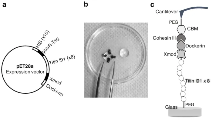
1. Transform the BL21 competent cells with the chimeric pET28a plasmid (see Note 5, Figure 3-a) according to the protocol provided by the competent cell manufacturer. 2. Using proper aseptic technique spread 50-100 µL of transfected cells onto an LB/agar
selection plate containing kanamycin (50 µg/mL) and incubate overnight at 37°C. 3. Select a bacterial colony from the agar plate and grow it up in a 20 mL LB broth +
kanamycin (50 µg/mL) for 4-6 hours in a shaking incubator at 37°C (250 rpm) or until O.D. at 600 nm reaches 1.0.
4. Expand the culture by growing 10 mL of starting culture in 1 L LB broth + kanamycin + 2 mM CaCl2 in 2.8 L Fernbach culture flask (see Note 1). Grow in a shaking incubator at
5. Induce protein expression by adding IPTG to a final concentration of 0.3 mM. Induction should be carried out overnight at 20 °C in a shaking incubator (200 rpm).
6. After induction harvest the cells by centrifugation (i.e. 3500 x g for 15 min) and gently resuspend the cells in 5 mL Lysis Buffer.
7. Add PMSF to a final concentration of 1 mM (see Note 6) and lyse the cells with a probe-type sonicator (place the sample in an ice bath, and use three cycles of 30 s bursts at 75% output amplitude and 30 s pauses to allow for heat dissipation and cooling).
8. Add DNase and MgCl2 at a final concentration of 10 µg/ml and 2 mM, respectively (see
Note 7). Add Triton X-100 at a final concentration 0.1% (see Note 8). Solubilize the
protein by shaking the suspension for 30 mins at 4°C.
9. Centrifuge the crude cell extract at 10,000 x g at 4°C for 45 min to remove cell debris. 10. Collect the supernatant (without touching the pellet) and mix it with 1 ml of Ni2+-NTA
affinity resin that has been already equilibrated with the Lysis Buffer (see Note 9). 11. Incubate the mixture on an end-ever-end shaker for 90 min at 4°C to allow binding of the
His-tagged protein (see Note 8).
12. Wash the resin with 5 mL Wash Buffer in order to decrease the unspecific adsorption of contaminating proteins. Repeat the washing step at least 3 times (see Note 9).
13. Elute the His-tagged protein 3 times with 0.5 mL Elution Buffer (see Note 9).
14. To remove the imidazole, dialyze the purified protein solution against 0.5 L of dialysis buffer for 1 h (use 10K MWCO membranes) at room temperature to speed-up diffusion. Change the dialysis buffer and dialyze overnight at 4°C. Analyze all fractions by
SDS-3.1.2 Surface functionalization
1. Rinse the glass surfaces and silicon nitride cantilevers with acetone for 10 minutes. (see
Notes 10-12)
2. If necessary (in case they are used) immerse the glass surfaces in a mixture of sulfuric acid (H2SO4) (75%) and hydrogen peroxide (H2O2) (25%) (so-called piranha solution) for 30
minutes. (see Notes 13-15)
3. Rinse the glass surfaces by dipping into ~ 1ml milli-Q water in a 24-well tissue culture plate (5 times)
4. Dry the glass surfaces and cantilevers with a gentle flow of N2
5. Clean glass surfaces and silicon nitride cantilevers with plasma cleaner 80 W power under oxygen for 5 minutes at 0.6 mbar.
6. Silanize the glass surfaces and cantilevers with 5% (3-aminopropyl)-dimethyl-ethoxysilane (3-APDMES) in EtOH for 10 minutes at room temperature. (see Notes 16-18)
7. Rinse the glass surfaces and cantilevers in analytical grade ethanol (more than 99.9% purity),
8. Bake the glass surfaces and cantilevers at 80°C for ~1 hour for curing. (see Note 19) 9. Immerse immediately the glass surfaces and cantilevers in PBS pH:9 and incubate
overnight at 4°C. This process is necessary to deprotonate the amino-groups on the surface of cover slips and cantilevers to help amide-bond formation with the NHS-ester group of the linker. (see Notes 20-21)
10. Rinse the glass surfaces and cantilevers by dipping into ~ 1 ml milli-Q water in a 24-well tissue culture plate (5 times)
11. Incubate the glass surfaces and cantilevers in ~5mM NHS-PEG-Maleimide in PBS pH:7.2 for 1 hour at room temperature to PEGylate the amino functionalized sides of the glass surfaces. In order to coat more than one surfaces and/or cantilevers with limited amount of solutions, we recommend to place them as illustrated in Figure 3-b.
12. Rinse the glass surfaces and cantilevers by dipping into ~ 1 ml milli-Q water in a 24-well tissue culture plate (5 times)
13. Incubate the PEGylated glass surfaces and cantilevers in 20 mM coenzyme A in coupling buffer 50 mM Na2PO4, 50 mM NaCl 10 mM EDTA pH7.2 for ~1 hour at room
temperature.
14. Rinse the glass surfaces and cantilevers by dipping into ~ 1 ml milli-Q water in a 24-well tissue culture plate (5 times) to remove unbound CoA.
15. Incubate the glass surfaces with ~100µg/mL ybbR-8x(titin)-XMod-dockerin in the reaction buffer 50 mM Hepes-NaOH, pH 7.5, 20 mM MgCl2 and 1mM CaCl2 in presence 1 µM Sfp
for 1 hour at room temperature. This process enables covalent immobilization of protein via Sfp-catalyzed ligation of coenzyme A and the ybbR-tags. (see Notes 22-23)
16. Incubate the cantilevers with ~100µg/mL ybbR-Cohesin-III in the reaction buffer 50 mM Hepes-NaOH, pH 7.5, 20 mM MgCl2 in presence 1 µM Sfp for 1 hour at room
temperature.
17. Rinse the functionalized glass surfaces and cantilevers with measurement buffer (PBS pH 7.2) and store in measurement buffer at 4°C until the measurements. (see Note 24). The final experimental design of the molecules is illustrated in Figure 3-c.
3.2 High-speed force spectroscopy (HS-FS)
FS measurements compose of three major steps: calibration of AFM cantilevers, FS measurements, and data processing and analysis. The detailed procedures of each steps are explained in sections 3.3.1-3.
3.2.1 Calibration of AFM cantilevers
In force spectroscopy, as the AFM cantilever deflects due to the interaction forces between the tip and the sample surface, the angle of the deflected laser beam changes, which translates into a difference between currents in the quadrants of the photodiode. The photodiode signal is in volts. In order to convert this signal into units of force the spring constant of the cantilever (𝑘) and the deflection sensitivity (also known as invOLS, inverse of the optical lever sensitivity, in nm/V) of the detection system must be calibrated before measurements [36]. The available techniques used in AFM to calibrate the cantilevers can be classified into two classes: contact-based and contact-free methods. In the contact based method the invOLS is determined by acquiring a force-distance curve on a stiff surface in liquid and then the cantilever spring constant is calculated by thermal fluctuations of the cantilever in liquid using the equipartition theorem [37,38]. In the non-contact method, the invOLS is determined using the thermal fluctuations in liquid together with a priori knowledge of the spring constant. Non-contact methods have various advantages: 1) the spring constant calibration is
independent of the determination of detector sensitivity (invOLS) minimizing propagation of errors, and 2) the invOLS determination does not require the acquisition of force curves on a hard substrate, preventing damaging the cantilever tip or the coating. Thus, we recommend using non-contact
methods. Sader method [39,40] is one of the non-contact methods to calibrate the spring constant of the cantilevers in air, which can be easily implemented in any AFM system, without any additional
equipment. The method uses the measured plan view dimensions of the cantilever, its resonance frequency and quality factor (𝑄) in air (see Notes 25-26), and the physical properties of ambient fluid (density and viscosity). Then the invOLS value can be calculated by using this spring constant and the
power spectral density of the thermal fluctuations in liquid [41,42]. The procedure for spring constant and invOLS calibration using the non-contact method is as follows:
1. Mount the cantilever on the cantilever holder.
2. Focus the laser beam at the very end of the cantilever where the tip is positioned trying to maximize the sum signal on the photodiode.
3. Adjust the position of the reflected beam to the center of the bi-segmented photodiode (zero horizontal deflection).
4. Acquire and save the thermal fluctuation spectrum of the cantilever. (see Note 27) 5. Extract the resonance frequency and the quality factor from the power spectral density
(PSD) of the thermal fluctuation response of a cantilever (See Figure 4-a).
6. Calculate the spring constant of the cantilever using Sader formula by using measured width and length of the cantilever (using optical or electron microscopy). (see Notes
25-26)
7. After functionalization of the cantilever, prior to engaging the cantilever on the surface, repeat Steps 2-5 and record and save the thermal fluctuation spectrum in liquid.
8. Using the calculated spring constant at Step 6 and the PSD in liquid (See Figure 4-b), determine the invOLS value.
[Place Figure 4 here].
3.2.2 Force Spectroscopy Measurements
After calibration and functionalization of the AFM cantilever, HS-FS measurements can be performed according to the detailed procedure described below.
1. Clean the cantilever holder by rinsing with Alconox, de-ionized water, acetone, de-ionized wa-ter, ethanol, de-ionized water in the given order.
2. Dry the cantilever holder head with dustless tissue and if possible blow some air or an inert gas to further clean the chamber.
3. Mount the cantilever on the cantilever holder under microscope with the help of clean stainless-steel tweezers.
4. Immediately fill the chamber with measurement buffer to prevent the functionalized cantilever to dry up, as this may damage the linked biomolecule. We recommend filling the chamber with the measurement buffer prior to mounting the cantilever where this will prevent any drying up possibilities. If the cantilever holder does not have a pool, add a drop of buffer.
5. Mount the cantilever holder head on the setup and adjust the connections
6. Focus the laser beam at the end of the cantilever where the tip is located trying to maximize the sum signal on the photodiode.
7. Clean the surface of the piezo located on the scanner of HS-AFM with a dustless tissue.
8. Immobilize the glass rod on the piezo using glue, nail polish or vacuum grease (we recommend vacuum grease for the sake of operational simplicity and to prevent exposure to glue or nail polish chemicals). In case you are using cover slips as a coated surface, place the cover slip on top of the glass rod with vacuum grease.
9. Immediately add a drop of measurement buffer (PBS) on the surface to prevent drying up. 10. Immediately place the sample holder (scanner) on the AFM setup by carefully dipping the
sam-ple surface into the chamber where the cantilever is mounted.
11. Align the coated surface on the cantilever, ensuring that the tip is sufficiently away from the surface (at least 20 µm).
13. Adjust the position of the reflected beam near the center of the segmented photodiode (zero hor-izontal deflection).
14. Acquire the thermal fluctuation spectrum of the cantilever in liquid away from the surface to calibrate the invOLS. (see Note 27)
15. Determine the invOLS using the known spring constant as determined in section 3.2.1. 16. Turn on the closed loop feedback on and adjust the set-point.
17. Engage the surface on the cantilever with the feedback on to make a slight contact or close enough to make contact manually. (see Note 28)
18. Turn off the feedback control, as the HS-FS measurements will be performed without a feed-back signal in order to be able to reach high velocities.
19. Start acquiring force-distance curves ensuring that the tip and the surface gets in contact; follow steps 20-25.
20. Approach the surface to the tip at ~1 µm/s until the required force is reached (<300pN). 21. Maintain this force for the desired contact time. (see Note 29)
22. Retract to initial position with constant velocity.
23. Move within the XY plane to probe fresh regions and prevent surface degradation.
24. Repeat the cycle (a to d) until a satisfactory amount of unbinding/unfolding force-distance curves are collected (50–100 successful events per velocity).
25. Repeat the force-distance data collection at different velocities logarithmically spaced, covering the widest possible range (usually from ~10 nm/s to ~10 mm/s) for dynamic force spectroscopy (DFS) analysis.
3.2.3 Data Processing and Analysis
events of 5-10% (sometimes up to 50%). The specific unfolding forces are extracted by inspecting the individual force-extension curves. However, considering the large number of data collected during the experiments and the low probability specific single-molecule unfolding events, an automated or semi-automated data processing tool is required. Most of the commercially available AFM equipment provides their own software developed to process the force-distance curves in a semi-automated fashion. However, we recommend writing one’s own tool especially if you are using an in-house developed HS-FS data acquisition software. Designing a molecular complex with a well-defined fingerprint of unfolding mechanism or using linkers with known unfolding or extension profile, such as PEG, assists to automated data processing.
The 8x(titin I91)-Xmod-Dock/Coh-CBM complex provides a characteristic unfolding of single domains followed by an unbinding of dockerin-cohesion III complex fingerprint shown in Figure 5, facilitating the recognition of successful events. A HS-FS raw data processing should contain the following steps.
1. Take a segment (around 10-20%) of the retraction curves from the end where the cantilever moves freely from any interaction with the surface.
2. If necessary, correct the optical interference by extracting the periodic interference signal from the force-distance data. (see Note 30)
3. Correct the force offset (baseline) using the mean force recorded in the segment defined in 1 by fitting a straight line to this part of the curve which will give the baseline. (see Note 31)
4. Calculate the relative tip displacement (piezo movement minus deflection, z–d). (see Note 32) 5. Determine the instantaneous velocity of the tip at each point by computing numerically the first
derivative of the relative tip displacement over time.
6. If necessary, correct the recorded force trace at each point by multiplying the instantaneous ve-locity by the viscous drag coefficient. (see Note 33)
7. Identify the point of contact. (see Note 34)
8. Detect the peaks in the retract profile automatically. (see Note 35)
9. Extract the specific unbinding/unfolding events by differentiating them from the non-specific adhesions. (see Note 36)
10. Determine the unfolding force. The unfolding force is the peak height, the difference between the peak point and the baseline.
11. Determine the loading rate by fitting a first order polynomial to a short time interval (corre-sponding to 1-3 nm) just before the rupture event in the force-time plot.
12. If force measurements span over various velocities, pool events by loading rate intervals, calcu-late histograms for each interval and determine the most probable unfolding force and median loading rate.
13. Extract the kinetic parameters, dissociation rate at zero force 𝑘%&& and the distance to the transition state 𝑥( of the unfolding energy landscape fitting a theoretical model describing the dependence of unfolding force and loading rate. (see Note 37)
[Place Figure 5 here].
4 Notes
1. Buffers and bacterial culture media should include calcium, which is necessary for the proper folding of cellulosome ultrastable complex proteins (cohesin and dockerin). 2. Imidazole concentration might need to be tuned for optimal washing.
3. The vertical motion of the sample stage is performed using a miniature multilayer piezoelectric actuator of dimensions 3 x 2 x 2 mm3 (PL033.33, Physik Instrumente,
The use of short AFM cantilevers (See Figure 2) requires focusing the laser beam (808nm, Newport) with a 20x optical microscope objective (ELWD, Nikon) with long working distance into a spot of ~3 µm diameter. The reflected beam is tracked using a 15 MHz bandwidth photodiode (MPR-1 AFM, Graviton).
The HS-FS setup is controlled with in-house built software based on Labiew using a multichannel analog to digital converter with maximum acquisition rate of 100
megasamples per second and channel. This allows control of the drive piezo displacement and acquisition of the cantilever deflection signal (PXI-5122, National Instruments). In this system, the cantilever is mounted facing up in a holder featuring a liquid pool of ~150 µL. The scanner with the sample support is mounted on top facing down (See Figure 1).
4. Short cantilevers are the most essential part of HS-AFM as they allow attaining µs-time resolution with a relatively low spring constant (0.1-0.6 N/m). There are mainly two companies that produce HS-AFM cantilevers Olympus (Olympus) and Nanoworld (Switzerland). To allow functionalization with the protocol described in this chapter (section 3.1-2), a cantilever tip of silicon or silicon nitride is required. Nanoworld cantilevers (USC-F1.2-k0.15 or USC-F1.5-k0.6) are made of quartz and feature an electron beam deposition (EBD) tip, thus not convenient to be functionalized with the protocol below. Olympus cantilevers (AC10DS, 2µmx8µmx0.1µm, Au backside coated, nominal spring constant 0.1N/m) are made of silicon nitride and feature a bird beak shape tip (See Figure 2), made also of silicon nitride and, thus, suitable for functionalization with the protocol described here. Note that Olympus commercializes a version of AC10
cantilevers featuring an electron beam deposited carbon tip (AC10FS). This type is not suitable for functionalization using the protocol described here.
5. Titin concatamer construct was assembled by standard molecular biology methods using polymerase chain reaction (PCR). ybbR-tag and Xmod-dockerin III domains were added at the N- and C-terminus of an 8x titin I91 domain concatamer, respectively. The PCR
product was purified and ligated to pET28a vector (See Figure 3-a) for transformation and protein expression in E. Coli BL21 strain. The expected weight of the encoded protein is about 109 kDa.
6. To protect the integrity of the protein from multiple proteases you may consider adding an EDTA-free protease inhibitor cocktail in addition to PMSF.
7. During sonication, nucleic acids are expected to undergo mechanical breakdown by
hydrodynamic shearing. RNase treatment of RNA (which is chemically unstable compared to DNA) is therefore unnecessary.
8. DNase and X-Triton will reduce the lysate viscosity and prevent aggregate formation, respectively.
9. Affinity resin manufacturers usually provide their products with an optimized, step-by-step protocol. We recommend you to integrate our recommendations to this material.
10. Glass cover slips are recommended for better functionalization.
11. Since cantilevers are quite small it is a difficult task to handle them and it is common to lose some of them during the whole coating process. Thus, we recommend functionalizing more than one cantilever for each experiment. In addition, it is recommended to check whether the cantilevers on the chip are intact and undamaged before starting the functionalization protocol. If you coat more than one probe simultaneously, label the probes before calibration. A tungsten or diamond pen may be used for that.
to prevent corrosion and should be performed under well-ventilated hood.
13. The mixing process of H2O2 and H2SO4 is a highly exothermic reaction. In order to avoid
any boiling or splashing, H2O2 must be mixed with H2SO4, SLOWLY. The solution itself is
highly explosive and hazardous, therefore the necessary safety precautions must be followed. Piranha solution cannot be stored for future use.
14. Since the piranha solution is highly corrosive, only glass or Teflon tools must be used while working with piranha solution.
15. The cantilevers should not be cleaned with piranha solution because they easily flip and break and it may damage the gold coating.
16. It is always good practice to put the larger volume component first and then the smaller volume component. Therefore, EtOH should be first put into the pyrex/glass petri dish and then 3-APDMES and should be mixed well by pipetting several times.
17. From now on, since only one side of the glass surfaces is treated, attention should be paid to use always the same side of the glass surfaces.
18. This 3-APDMES solution is very hygroscopic and can hydrolyze very quickly. In order to prevent air contact, Argon should be purged onto 3-APDMES bottle immediately and the bottle should be sealed properly with parafilm after purging Argon. We also recommend purchasing the solution in small volumes.
19. In order to allow evaporation but prevent contaminations the glass petri dish should be left semi-open in the oven.
20. Amino-functionalized surfaces can be stored for several days in the PBS buffer at alkaline pH solution at 4°C. If the cantilevers need to be stored more than few days, we recommend storing them dried under Argon.
21. Handling small coverslips and/or glass rods for functionalization might be difficult. To reduce the amount of protein used and to prevent evaporation, sandwiching a protein drop between two coverslips or between the coverslip and a clean surface (like parafilm, common in immunostaining) is a useful strategy.
22. The final reaction solution should contain 20mM MgCl2 for better functionalization. Thus,
necessary amount of MgCl2 should be added into Sfp solution before use.
23. Usually the stock solution of Sfp is 10 µM in 50 mM Hepes-NaOH, pH7.5 10 mM MgCl2. The necessary amount of Sfp + MgCl2 mixture should be added onto the cantilevers after
the protein solution to achieve 1 µM of Sfp in final incubation solution and mixed well via pipetting several times.
24. For better efficiency, it is recommended to use the coated surfaces within 2 days. 25. Sader method is valid only for high Q-factor cantilevers. This is the case of AC10DS
cantilevers in air.
26. Sader and co-workers initiated a web-based platform for spring constant calibration, called the Global Calibration Initiative (GCI). Using this portal, any AFM user can upload the calibration parameters (spring constant, resonance frequency and Q-factor) of their own cantilevers, establishing a global database [43]. The assessment of the uploaded data from individual users facilitates calculation of a universal coefficient, called 𝐴-coefficient, for each specific cantilever geometry which completes the functional relation between the spring constant 𝑘 , the resonance frequency (𝑓+) and the quality factor (𝑄) measured in
air. The portal also allows correction of the spring constant using the globally calculated A-coefficient. The spring constant determination via the GCI becomes more and more
27. The cantilever must be sufficiently away from any surface, at least 50 µm.
28. In this step, it is recommended to use a set-point ~10% below the zero-deflection value in order to minimize the applied force and time in contact. This step allows getting close enough to the cantilever, for then finish the actual engagement manually.
29. The adhesion frequency (fraction of successful unfolding events) has to be kept below 30%, preferable 10% in general, as low adhesion frequency ensures that the majority of the unfolding events are due to single molecule unfolding. However, given the specific
fingerprint of the proposed protein construct, this success rate can be higher provided no multiple events are observed. Moreover, the contact time between adhering surfaces and/or the protein densities on the surfaces can be adjusted to control the adhesion frequency. A typical contact time using the proposed protocol is about 100 ms, but for higher velocities, longer contact time may be needed.
30. In order to correct the periodic interference signal, a sinusoidal relation to the force-distance data with the correct amplitude and period can be fit to the data. More advanced functions have been proposed (see, for example, supplementary material of ref. [19]). In this work, no correction was necessary.
31. Ideally, after the last rupture event, the signal should be a straight, flat line with a certain noise level caused by thermal fluctuations until the end of the piezo movement. A signal presenting a slope is often observed on tip moving AFM systems and long z-ranges. This may be corrected by fitting and removing a straight line.
32. The actual tip displacement is different than the piezo movement because of the bending of the cantilever due to the viscous forces acting on the cantilever caused my surrounding fluid movement.
33. Due to the viscous drag force exerted on the cantilever caused by movement of the surrounding medium the baselines of the approach and retract traces can be shifted away from each other. The viscous drag force depends on the retract velocity, the separation between the tip and the surface and the cantilever geometry. At very high velocities, the viscous drag effect should be corrected [44,45]. The difference in force between approach and retract baselines where the cantilever moves freely will give the viscous drag force at the corresponding velocity. The viscous drag coefficient (b) can be extracted from the linear relation between the viscous drag force and the relative tip velocity.
34. The intersection of the smoothed retract trace and the extrapolation of the corrected baseline is a way to determine the point of contact. Another method involves detecting the first data point that changes from positive to negative deflection (starting from the contact region).
35. Sharp jumps after a stretching regime in the force-distance profile are candidates for rupture events of protein-ligand complexes or single domain unfolding. In order to locate the sharp jumps, one can calculate the first derivative of the deflection within a certain interval which provides the slope of the curve within that interval and large slope values reflect sharp jumps. Defining a threshold for the slope is commonly used to locate inflection points and thereby the location of the peaks. Any other peak detection algorithms can also be applied.
36. Often, non-specific adhesion occurs between the tip and the coated surface. Using linker molecules like PEG with a known length will help to prevent unspecific binding.
37. The Bell model [49] is the first and still the most conventional phenomenological model used to describe the rupture of molecular bonds under an external mechanical force. The
(so-called Bell-Evans model) [50]. This model describes a linear relation between the rupture force and the logarithm of the loading rate. There are also other models which predicts a nonlinear dependence of the most probable rupture force and the logarithm of the loading rate by taking into account the modulation of the distance between initial and transient state [51], the possibility of rebinding [52], the intrinsic properties of the
molecule and the cantilever [53,54] and to extend the applicable dynamic range [55,56].
Acknowledgement
This work was supported by Agence National de la Recherche grants BioHSFS ANR-15-CE11-0007 and ANR-11-LABX-0054 (Labex INFORM). A.M. was supported by a Long Term EMBO Fellowship (ALTF 1427-2014) and a Marie Curie Action (MSCA-IF-2014-EF-655157). We thank Michael Nash and Wolfgang Ott for sharing the XMod-dockerin-III and cohesin-III plasmids and for technical assistance.
5 References
1. Kubelka J, Hofrichter J, Eaton WA (2004) The protein folding ‘speed limit’. Current opinion in structural biology 14 (1):76-88
2. Alberts B, Bray D, Lewis J, Raff M, Roberts K, Watson JD (1994) Molecular Biology of the Cell. 3rd edn. Garland Publishing, New York,
3. Bryngelson JD, Onuchic JN, Socci ND, Wolynes PG (1995) Funnels, pathways, and the energy landscape of protein folding: A synthesis. Proteins: Structure, Function, and Bioinformatics 21 (3):167-195. doi:10.1002/prot.340210302
4. Kellermayer MsSZ, Smith SB, Granzier HL, Bustamante C (1997) Folding-Unfolding Transitions in Single Titin Molecules Characterized with Laser Tweezers. Science 276 (5315):1112-1116.
doi:10.1126/science.276.5315.1112
5. Rief M, Gautel M, Oesterhelt F, Fernandez JM, Gaub HE (1997) Reversible Unfolgind of Individual Titin Immunoglobulin Domains by AFM. Science 276:1109-1112. doi:10.1126/science.276.5315.1109 6. del Rio A, Perez-Jimenez R, Liu R, Roca-Cusachs P, Fernandez JM, Sheetz MP (2009) Stretching Single Talin Rod Molecules Activates Vinculin Binding. Science 323 (5914):638-641.
doi:10.1126/science.1162912
7. Johnson CP, Tang H-Y, Carag C, Speicher DW, Discher DE (2007) Forced Unfolding of Proteins Within Cells. Science 317 (5838):663-666. doi:10.1126/science.1139857
8. Dobson CM (2003) Protein folding and misfolding. Nature 426 (6968):884-890
9. Schwaiger I, Kardinal A, Schleicher M, Noegel AA, Rief M (2004) A mechanical unfolding intermediate in an actin-crosslinking protein. Nat Struct Mol Biol 11 (1):81-85
10. Marszalek PE, Lu H, Li H, Carrion-Vazquez M, Oberhauser aF, Schulten K, Fernandez JM (1999) Mechanical unfolding intermediates in titin modules. Nature 402 (November):100-103.
doi:10.1038/47083
11. Oberhauser AF, Hansma PK, Carrion-Vazquez M, Fernandez JM (2001) Stepwise unfolding of titin under force-clamp atomic force microscopy. Proceedings of the National Academy of Sciences of the United States of America 98 (2):468-472
12. Oesterhelt F, Oesterhelt D, Pfeiffer M, Engel A, Gaub HE, Müller DJ (2000) Unfolding Pathways of Individual Bacteriorhodopsins. Science 288 (5463):143-146. doi:10.1126/science.288.5463.143
14. Neupane K, Foster DA, Dee DR, Yu H, Wang F, Woodside MT (2016) Direct observation of transition paths during the folding of proteins and nucleic acids. Science 352 (6282):239-242 15. Hughes ML, Dougan L (2016) The physics of pulling polyproteins: a review of single molecule force spectroscopy using the AFM to study protein unfolding. Rep Prog Phys 79 (7):076601. doi:10.1088/0034-4885/79/7/076601
16. Ando T, Kodera N, Naito Y, Kinoshita T, Furuta Ky, Toyoshima YY (2003) A High-speed Atomic Force Microscope for Studying Biological Macromolecules in Action. ChemPhysChem 4 (11):1196-1202. doi:10.1002/cphc.200300795
17. Viani MB, Schaffer TE, Chand A, Rief M, Gaub HE, Hansma PK (1999) Small cantilevers for force spectroscopy of single molecules. J Appl Phys 86:2258-2262
18. Rico F, Gonzalez L, Casuso I, Puig-vidal M, Scheuring S (2013) High-Speed Force Spectroscopy Molecular Dynamics Simulations. Science 342 (November):741-743. doi:10.1126/science.1239764 19. Yu H, Siewny MG, Edwards DT, Sanders AW, Perkins TT (2017) Hidden dynamics in the unfolding of individual bacteriorhodopsin proteins. Science 355 (6328):945-950. doi:10.1126/science.aah7124 20. Rigato A, Miyagi A, Scheuring S, Rico F (2017) High-frequency microrheology reveals
cytoskeleton dynamics in living cells. Nature Physics
21. Edwards DT, Faulk JK, Sanders AW, Bull MS, Walder R, LeBlanc MA, Sousa MC, Perkins TT (2015) Optimizing 1-mus-Resolution Single-Molecule Force Spectroscopy on a Commercial Atomic Force Microscope. Nano Lett 15 (10):7091-7098. doi:10.1021/acs.nanolett.5b03166
22. Rico F, Gonzalez L, Casuso I, Puig-Vidal M, Scheuring S (2013) High-Speed Force Spectroscopy Unfolds Titin at the Velocity of Molecular Dynamics Simulations. Science 342 (6159):741-743. doi:10.1126/science.1239764
unfolding of individual bacteriorhodopsin proteins. Science 355 (6328):945-950. doi:10.1126/science.aah7124
24. Kassies R, van der Werf KO, Bennink ML, Otto C (2004) Removing interference and optical feedback artifacts in atomic force microscopy measurements by application of high frequency laser current modulation. Rev Sci Instrum 75 (3):689-693. doi:doi:http://dx.doi.org/10.1063/1.1646767 25. Carrion-Vazquez M, Oberhauser AF, Fowler SB, Marszalek PE, Broedel SE, Clarke J, Fernandez JM (1999) Mechanical and chemical unfolding of a single protein: A comparison. Proceedings of the National Academy of Sciences 96 (7):3694-3699. doi:10.1073/pnas.96.7.3694
26. Ando T, Kodera N, Takai E, Maruyama D, Saito K, Toda A (2001) A high-speed atomic force microscope for studying biological macromolecules. Proceedings of the National Academy of Sciences 98 (22):12468-12472. doi:10.1073/pnas.211400898
27. Zakeri B, Fierer JO, Celik E, Chittock EC, Schwarz-Linek U, Moy VT, Howarth M (2012) Peptide tag forming a rapid covalent bond to a protein, through engineering a bacterial adhesin. Proc Natl Acad Sci U S A 109 (12):E690-697. doi:10.1073/pnas.1115485109
28. Otten M, Ott W, Jobst MA, Milles LF, Verdorfer T, Pippig DA, Nash MA, Gaub HE (2014) From genes to protein mechanics on a chip. Nat Methods 11 (11):1127-1130. doi:10.1038/nmeth.3099 29. Schoeler C, Malinowska KH, Bernardi RC, Milles LF, Jobst MA, Durner E, Ott W, Fried DB, Bayer EA, Schulten K (2014) Ultrastable cellulosome-adhesion complex tightens under load. Nature Communications 5
30. Pippig DA, Baumann F, Strackharn M, Aschenbrenner D, Gaub HE (2014) Protein-DNA chimeras for nano assembly. ACS Nano 8 (7):6551-6555. doi:10.1021/nn501644w
doi:10.1021/ja4056382
32. Otten M, Ott W, Jobst MA, Milles LF, Verdorfer T, Pippig DA, Nash MA, Gaub HE (2014) From genes to protein mechanics on a chip. Nat Meth advance online publication. doi:10.1038/nmeth.3099 http://www.nature.com/nmeth/journal/vaop/ncurrent/abs/nmeth.3099.html - supplementary-information 33. Zimmermann JL, Nicolaus T, Neuert G, Blank K (2010) Thiol-based, site-specific and covalent immobilization of biomolecules for single-molecule experiments. Nat Protoc 5 (6):975-985.
doi:10.1038/nprot.2010.49
34. Yin J, Lin AJ, Golan DE, Walsh CT (2006) Site-specific protein labeling by Sfp phosphopantetheinyl transferase. Nat Protoc 1 (1):280-285. doi:10.1038/nprot.2006.43
35. Durner E, Ott W, Nash MA, Gaub HE (2017) Post-Translational Sortase-Mediated Attachment of High-Strength Force Spectroscopy Handles. ACS Omega 2 (6):3064-3069.
doi:10.1021/acsomega.7b00478
36. Zhang X, Rico F, Xu AJ, Moy VT (2009) Atomic Force Microscopy of Protein–Protein Interactions. In. Springer US, New York, NY, pp 555-570. doi:10.1007/978-0-387-76497-9_19 37. Hutter JL, Bechhoefer J (1993) Calibration of atomic-force microscope tips. Rev Sci Instrum 64 (7):1868-1873
38. Butt HJ, Jaschke M (1995) Calculation of thermal noise in atomic force microscopy. Nanotechnology 6:1-7
39. Sader JE, Chon JWM, Mulvaney P (1999) Calibration of rectangular atomic force microscope cantilevers. Review of Scientific Instruments 70 (10):3967-3969. doi:10.1063/1.1150021
40. Sader JE, Larson I, Mulvaney P, White L (1995) Method for the calibration of atomic force microscope cantilevers. Rev Sci Instrum 66 (7):3789-3798
41. Higgins MJ, Proksch R, Sader JE, Polcik M, Mc Endoo S, Cleveland JP, Jarvis SP (2006)
Noninvasive determination of optical lever sensitivity in atomic force microscopy. Review of Scientific Instruments 77 (1):1-5. doi:10.1063/1.2162455
42. Schillers H, Rianna C, Schäpe J, Luque T, Doschke H, Wälte M, Uriarte JJ, Campillo N, Michanetzis GPA, Bobrowska J, Dumitru A, Herruzo ET, Bovio S, Parot P, Galluzzi M, Podestà A, Puricelli L, Scheuring S, Missirlis Y, Garcia R, Odorico M, Teulon J-M, Lafont F, Lekka M, Rico F, Rigato A, Pellequer J-L, Oberleithner H, Navajas D, Radmacher M (2017) Standardized
Nanomechanical Atomic Force Microscopy Procedure (SNAP) for Measuring Soft and Biological Samples. Scientific Reports 7 (1):5117. doi:10.1038/s41598-017-05383-0
43. Sader JE, Borgani R, Gibson CT, Haviland DB, Michael J, Kilpatrick JI, Lu J, Mulvaney P, Shearer CJ, Ashley D (2016) A virtual instrument to standardise the calibration of atomic force microscope cantilevers. arXiv. doi:10.1063/1.4962866
44. Janovjak H, Struckmeier J, Müller DJ (2005) Hydrodynamic effects in fast AFM single-molecule force measurements. European Biophysics Journal 34 (1):91-96. doi:10.1007/s00249-004-0430-3 45. Alcaraz J, Buscemi L, Puig-de-Morales M, Colchero J, Baro A, Navajas D (2002) Correction of microrheological measurements of soft samples with atomic force microscopy for the hydrodynamic drag on the cantilever. Langmuir 18 (3):716-721
46. Bustamante C, Marko JF, Siggia ED, Smith S (1994) Entropic elasticity of lambda-phage DNA. Science (New York, NY) 265 (1994):1599-1600. doi:10.1126/science.8079175
47. Ortiz C, Hadziioannou G (1999) Entropic elasticity of single polymer chains of poly(methacrylic acid) measured by atomic force microscopy. Macromol 32:780-787
49. Bell G (1978) Models for the specific adhesion of cells to cells. Science 200 (4342):618-627. doi:10.1126/science.347575
50. Evans E, Ritchie K (1997) Dynamic Strength of Molecular Adhesion Bonds. Biophys J 72:1541-1555. doi:10.1016/S0006-3495(97)78802-7
51. Dudko OK, Hummer G, Szabo A (2006) Intrinsic rates and activation free energies from single-molecule pulling experiments. Physical Review Letters 96 (10). doi:10.1103/PhysRevLett.96.108101 52. Friddle RW, Noy a, De Yoreo JJ (2012) Interpreting the widespread nonlinear force spectra of intermolecular bonds. Proceedings of the National Academy of Sciences 109 (34):13573-13578. doi:10.1073/pnas.1202946109
53. Evans E, Ritchie K (1999) Strength of a weak bond connecting flexible polymer chains. Biophys J 76 (5):2439-2447. doi:10.1016/S0006-3495(99)77399-6
54. Maitra A, Arya G (2010) Model accounting for the effects of pulling-device stiffness in the analyses of single-molecule force measurements. Phys Rev Lett 104 (10):108301.
doi:10.1103/PhysRevLett.104.108301
55. Bullerjahn JT, Sturm S, Kroy K (2014) Theory of rapid force spectroscopy. Nat Commun 5. doi:10.1038/ncomms5463
56. Hummer G, Szabo A (2003) Kinetics from nonequilibrium single-molecule pulling experiments. Biophys J 85 (1):5-15
Figure Captions
Figure 1. High speed force spectroscopy setup. The molecular construct of 8 concatanated titin I91
domains and the Xmod-dockerin III complex covalently attached to the support and the CBM-Cohesin III complex covalently attached to the tip (shown in the inset). NMR structure of titin monomer
(PDB:1TIT), crystal structure of Xmod-dockerin/Cohesin complex (PDB: 4IU3) and crystal structure of CBM (PDB:4B9F) are used to show the full complex used in the experiments.
Figure 2. Short AFM cantilever. (a) Olympus AC10DS chip from top and side view with its
Figure 3. DNA construct and cantilever and surface coating. (a) DNA construct for the
ybbR-titin8-XMod-dockerin chimera. Diagram showing the pET28a expression vector after insertion of the titin chimera. Histidine and ybbR tags where added upstream the titin 8x repeat. Xmod and dockerin III domain where added downstream. (b) Handling the AFM cantilevers during coating. (c) Schematic illustration of surface and cantilever coating with relevant molecules.
Figure 4. Contact free calibration of the spring constant and invOLS (a) Power spectral density
(PSD) of the thermal fluctuations of a cantilever (AC10DS) in air with the respective fit to cantilever's first mode. The spring constant determined using the Sader method was 0.11 N/m, the fitted resonance frequency and Q-factor were 1487 kHz and 35, respectively. (b) PSD of the thermal fluctuations of the same cantilever (AC10DS) in liquid with the respective fit to cantilever's first mode. The invOLS value was 76.5 nm/V, the fitted resonance frequency and Q-factor were 609 kHz and 1.3, respectively.
Figure 5. Example force-distance curves. (a) Rejected unfolding traces during data processing. The
unfolding curves which have unexpected unfolding events, such as, no dockerin-cohesin III unbinding at the last event (curves 1 and 4), less than eight titin unfolding peaks (curve 2), longer or shorter unfolded chain lengths (curve 3) should be rejected during data processing. (b) Accepted unfolding traces during data processing. In the curve 1, the Xmod domain unfolds before dockerin-cohesin III unbinding as also reported in [27].