HAL Id: ensl-00409366
https://hal-ens-lyon.archives-ouvertes.fr/ensl-00409366v3
Submitted on 4 Jan 2011
HAL is a multi-disciplinary open access
archive for the deposit and dissemination of
sci-entific research documents, whether they are
pub-lished or not. The documents may come from
teaching and research institutions in France or
abroad, or from public or private research centers.
L’archive ouverte pluridisciplinaire HAL, est
destinée au dépôt et à la diffusion de documents
scientifiques de niveau recherche, publiés ou non,
émanant des établissements d’enseignement et de
recherche français ou étrangers, des laboratoires
publics ou privés.
Midpoints and exact points of some algebraic functions
in floating-point arithmetic
Claude-Pierre Jeannerod, Nicolas Louvet, Jean-Michel Muller, Adrien
Panhaleux
To cite this version:
Claude-Pierre Jeannerod, Nicolas Louvet, Jean-Michel Muller, Adrien Panhaleux. Midpoints and
ex-act points of some algebraic functions in floating-point arithmetic. IEEE Transex-actions on Computers,
Institute of Electrical and Electronics Engineers, 2011, 60 (2), pp.228-241. �10.1109/TC.2010.144�.
�ensl-00409366v3�
Midpoints and Exact Points of Some Algebraic
Functions in Floating-Point Arithmetic
Claude-Pierre Jeannerod, Member, IEEE, Nicolas Louvet,
Jean-Michel Muller, Senior Member, IEEE, and Adrien Panhaleux
Abstract—When implementing a function f in floating-point arithmetic, if we wish correct rounding and good performance, it is important to know if there are input floating-point values x such that fðxÞ is either the middle of two consecutive floating-point numbers (assuming rounded-to-nearest arithmetic), or a floating-point number (assuming rounded toward #1 or toward 0 arithmetic). In the first case, we say that fðxÞ is a midpoint, and in the second case, we say that fðxÞ is an exact point. For some usual algebraic functions and various floating-point formats, we prove whether or not there exist midpoints or exact points. When there exist midpoints or exact points, we characterize them or list all of them (if there are not too many). The results and the techniques presented in this paper can be used in particular to deal with both the binary and the decimal formats defined in the IEEE 754-2008 standard for floating-point arithmetic.
Index Terms—Floating-point arithmetic, correct rounding, algebraic function.
Ç
1
I
NTRODUCTIONI
Na floating-point system that follows the IEEE 754-1985standard for radix-2 floating-point arithmetic [1], the user can choose an active rounding mode, also called rounding-direction attribute in the newly revised IEEE 754-2008 standard [5]: rounding toward$1, rounding toward þ1, rounding toward 0, and rounding to nearest, which is the default rounding mode. Given a real number x, we denote, respectively, by RDðxÞ, RUðxÞ, RZðxÞ, and RNðxÞ these rounding modes. Let us also recall that correct rounding is required by the above cited IEEE standards for the four elementary arithmetic operations (þ, $, &, and ') as well as for the square root: the result of an operation is said to be correctly rounded if for any inputs, its result is the infinitely precise result rounded according to the active rounding mode. We are interested here in facilitating the delivery of correctly rounded results for various simple algebraic functions that are frequently used in numerical analysis or signal processing.
Let us call midpoint for a floating-point format a number that is exactly halfway between two consecutive floating-point numbers of that format. Given a function f : IRd! IR
and a floating-point vector x, we say that fðxÞ is a midpoint of f if fðxÞ is a midpoint for that format.
Given f and x, the problem of computing RNðfðxÞÞ is closely related to the knowledge of the midpoints of the function f. Then, a common strategy (see [15] and [10, chapter 10]) for returning RNðfðxÞÞ is as follows:
Let us first compute an approximation f1, of accuracy !1,
to fðxÞ. If there are no midpoints of the considered floating-point format within distance !1 from f1, then necessarily
RNðfðxÞÞ ¼ RNðf1Þ. If on the contrary, there are such
midpoints within distance !1from f1, we can progressively
increase the quality of the approximations (that is, comput-ing an approximation f2of accuracy !2< !1, and so on) until
we are able to provide a correctly rounded result. The point is that this strategy may not terminate if the function f has midpoints. As a consequence, a correctly rounded imple-mentation of a given function f can be made more efficient if we know in advance that f admits no midpoints. If f admits midpoints, it is also very useful to know how to characterize them.
If now we consider one of the directed rounding modes (RD, RU, or RZ), the strategy that consists in progressively refining the approximations will not terminate if fðxÞ is a floating-point number. In this case, we say that fðxÞ is an exact point of the function f, and it is also very useful to know a characterization of these exact points when implementing f. Moreover, a characterization of the exact points of f can be used to set the “inexact” flag required by the IEEE standards [1], [5]. For example, for x=pffiffiffiffiffiffiffiffiffiffiffiffiffiffiffix2þ y2 in radix 2, our study
shows that this flag must always be raised except when x or y is zero, which can be detected easily.
In this paper, we present results on the existence of midpoints and exact points for some algebraic functions: beyond division, inversion, and square root, we study functions like the reciprocal square root 1= ffiffiffiyp , the 2D euclidean norm pffiffiffiffiffiffiffiffiffiffiffiffiffiffiffix2þ y2 and its reciprocal 1=pffiffiffiffiffiffiffiffiffiffiffiffiffiffiffix2þ y2, . C.-P. Jeannerod is with INRIA Rhoˆne-Alpes, LIP (UMR 5668
CNRS—ENS de Lyon—INRIA—UCBL), Universite´ de Lyon, 46 alle´e d’Italie, F69364 Lyon Cedex 07, France.
E-mail: [email protected].
. N. Louvet is with UCBL Lyon 1, LIP (UMR 5668 CNRS—ENS de Lyon—INRIA—UCBL), Universite´ de Lyon, 46 alle´e d’Italie, F69364 Lyon Cedex 07, France. E-mail: [email protected].
. J.-M. Muller is with CNRS, LIP (UMR 5668 CNRS—ENS de Lyon—INRIA—UCBL), Universite´ de Lyon, 46 alle´e d’Italie, F69364 Lyon Cedex 07, France. E-mail: [email protected]. . A. Panhaleux is with ENS Lyon—Universite´ de Lyon, LIP (UMR 5668
CNRS—ENS de Lyon—INRIA—UCBL), 46 alle´e d’Italie, F69364 Lyon Cedex 07, France. E-mail: [email protected].
Manuscript received 7 Aug. 2009; revised 24 Mar. 2010; accepted 19 Apr. 2010; published online 11 June 2010.
Recommended for acceptance by J. Bruguera, M. Cornea, and D. Das Sarma. For information on obtaining reprints of this article, please send e-mail to: [email protected], and reference IEEECS Log Number TCSI-2009-08-0374. Digital Object Identifier no. 10.1109/TC.2010.144.
and the 2D-normalization function x=pffiffiffiffiffiffiffiffiffiffiffiffiffiffiffix2þ y2. A part of
the results presented on division and square root have been known for some time in binary arithmetic; see, for instance, the pioneering work by Markstein [9], as well as studies by Iordache and Matula [6] and Parks [11]. Let us also recall the work by Lauter and Lefe`vre [8] on the function xy, which thus covers integer powers. We present these results for completeness, and extend some of them to other radices, in particular to radix 10.
Before going into further details, we introduce some definitions. A radix-", precision-p floating-point number x is either 0 or a rational number of the form
x¼ #X ) "ex$pþ1;
where X is a positive integer such that X < "p. If in
addition "p$1* X, then x ¼ #X ) "ex$pþ1 is called the
normalized representation of x, and the integers X and ex
are called, respectively, the integral significand and the exponent of x. We can, in fact, speak of the exponent for any nonzero real x: in radix ", it is the unique integer ex such
that "ex* jxj < "exþ1. On computing systems conforming to
the IEEE 754-2008 standard [5], the radix " is 2 or 10. Radix 16 is also sometimes used [12]. The exponent ex is
bounded: emin* ex* emax, where emin and emax are the
extremal exponents of the considered floating-point format. A nonzero number without a normal representation is said subnormal: all subnormal numbers have absolute value less than "emin.
Assuming that we are working with a radix-", preci-sion-p floating-point arithmetic, a midpoint is a rational number of the form
z¼ # Z þ 1=2ð Þ ) "ez$pþ1;
where Z is a nonnegative integer such that "p$1* Z < "p; if e
min< ez* emax;
0* Z < "p; if e
z¼ emin:
"
Such a number is exactly halfway between two consecutive floating-point numbers. The midpoints are the values where the function x7! RNðxÞ is discontinuous, as illustrated in Fig. 1 on a toy floating-point format ("¼ 2, p ¼ 3, emin¼ $1,
and emax¼ 1).
When using the implementation of a mathematical function in floating-point arithmetic, in most practical cases, the input and output precisions are the same. However, a user may, for example, wish to calculate the single-precision/binary32 number that is closest to the square root of a double-precision/binary64 floating-point number. For the sake of simplicity, we assume, in this paper, that the input and output precisions are the same. Moreover, we give our results assuming an unbounded exponent range, that is, under the hypothesis that no underflow nor overflow occurs. For that purpose, we define IF";p as the
set of the radix-", precision-p floating-point numbers, with an unbounded exponent range. Similarly, midpoints are restricted to the set
MM";p¼## ðZ þ 1=2Þ ) "ez$pþ1 :
Z2 NN; "p$1* Z < "p; e z2 ZZ$;
where ZZ denotes the set of integers and NN denotes the set f0; 1; 2; . . .g of nonnegative integers.
The purpose of this paper is, for the floating-point number systems and the algebraic functions mentioned above, to investigate whether these functions admit midpoints or exact points, and to characterize such midpoints and exact points when they exist. The results we obtain are for "¼ 2qwith q a
positive integer, and for "¼ 10, but in some cases, we managed to weaken these assumptions on ". Moreover, most of the examples proposed are based on the basic formats defined in the IEEE 754-2008 standard [5] that are briefly recalled below:
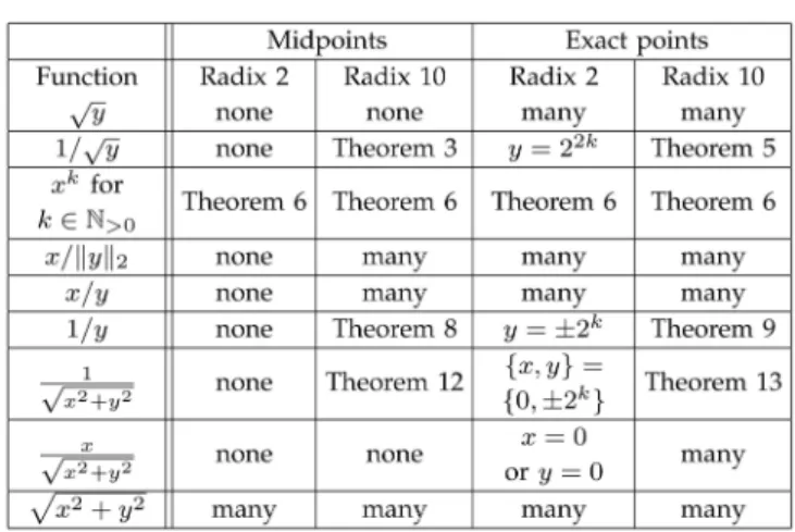
Table 1 summarizes the results presented in the paper. In this table, “many” indicates that the techniques we used did not allow us to find a simple characterization of the midpoints or of the exact points of the function, an exhaustive enumeration was impractical because of the too large number of cases to consider, and we have experimental evidence that the number of midpoints and/or exact points is
Fig. 1. The RNðxÞ function (radix " ¼ 2 and precision p ¼ 3).
TABLE 1
large. Most of the results displayed here for "¼ 2 are, in fact, obtained in a more general setting, namely, for "¼ 2q, where
q is a positive integer.
Note that since we considered an unbounded exponent range, subnormal floating-point numbers of the various IEEE 754-2008 formats can be written in normalized form. Hence, subnormal numbers are a subset of floating-point numbers with unbounded exponent range. This implies that the results presented in Table 1 remain unchanged when the inputs are subnormal numbers. If there are no exact points or midpoints for normal floating-point numbers with un-bounded exponent range for a given function, then mid-points or exact mid-points cannot occur if the inputs are subnormals. Similarly, if the exact points and midpoints are characterized by one of the theorems, assuming that the inputs are subnormals will only restrict the characterization of the theorem, without creating new possible exact points or midpoints.
However, some results presented in Table 1 change when we want to know if a given function outputs midpoints in the range of subnormal floating-point numbers. In radix 2, division admits midpoints in the subnormal range, as well as the function x=kyk2, while they have no midpoints in the
normal range. The square root function admits no midpoints, even in the subnormal range, for the square root of a floating-point number cannot be in the subnormal range. Although the results are not detailed in the paper, the techniques presented can be used to deal with midpoints in the subnormal range for the other functions listed in Table 1.
Outline.We start with extensions to radices 2qand 10 of
classical, radix-2 results for square roots (Section 2), recipro-cal square roots (Section 3), and positive integer powers (Section 4). In Section 5, we move to the function that maps a real x and a d-dimensional real vector y¼ ½yk,1*k*dto x=kyk2.
Here,k ) k2denotes the euclidean norm of vectors: kyk2¼ ffiffiffiffiffiffiffiffiffiffiffiffiffiffiffiffiffiffiffiffiffiffiffiffiffiffi y2 1þ ) ) ) þ y2d q :
The function x=kyk2 is interesting for it covers several important special cases, each of them being detailed in a subsequent section: for d¼ 1, division and reciprocal (Sections 6 and 7); for d¼ 2, reciprocal 2D euclidean norm 1=pffiffiffiffiffiffiffiffiffiffiffiffiffiffiffix2þ y2 and normalization of 2D vectors x=pffiffiffiffiffiffiffiffiffiffiffiffiffiffiffix2þ y2
(Sections 8 and 9). We comment on the 2D euclidean norm in Section 10.
Notation.Throughout the paper, the symbols QQ, IR, and NN>0denote the rational numbers, the real numbers, and the
positive integers, respectively. We write i for the complex number whose square is $1, and b)c and d)e for the usual floor and ceiling functions. Also, for x; y2 ZZ such that y6¼ 0, we use the standard notation x mod y ¼ x $ ybx=yc (see, for instance, Graham et al. [4, p. 82]).
2
S
QUARER
OOT2.1 Midpoints for Square Root
The following theorem can be viewed as a consequence of a result of Markstein [9, Theorem 9.4]. It says that the square root function has no midpoints, whatever the radix " is. A detailed proof is given here for completeness.
Theorem 1 (Markstein [9]). Let y2 IF";p be positive. Then,
ffiffiffi y p 62 MM
";p.
Proof.Let z¼pffiffiffiyand assume that z is in MM";p. Then, there
exist some integers Z and ez such that z¼ ðZ þ 1=2Þ )
"ez$pþ1 and "p$1* Z < "p. Using y¼ z2 and y¼
Y ) "ey$pþ1, we deduce that
4Y ) "ey$2ezþp$1¼ ð2Z þ 1Þ2: ð1Þ
Now, one may check that ez¼ bey=2c so that
ey$ 2ez¼ eymod 2; ð2Þ
which is nonnegative. Thus, for p- 1, the left-hand side of (1) is an even integer. This contradicts the fact that the right-hand side is an odd integer. tu 2.2 Exact Points for Square Root
We saw in the previous section that the square root function has no midpoints. The situation for exact points is just opposite: for a given input exponent, the number N of floating-point numbers having this exponent and whose square root is also a floating-point number grows essen-tially like "p=2. In this section, we make this claim precise for "¼ 2q(q2 NN
>0) and "¼ 10 by giving an explicit expression
for N in Theorem 2. To establish this counting formula, we need the following two lemmas:
Lemma 1.For a; b2 IR such that 0 * a * b, and c 2 NN>0, the
number of integer multiples of c that lie in ½a; bÞ is db=ce $ da=ce.
Proof.Let us write Na;bðcÞfor the number of integer multiples of c lying in½a; bÞ. Since 0 * a * b, the set ½0; bÞ is the union of the disjoint sets½0; aÞ and ½a; bÞ. Hence, Na;bðcÞ¼ N0;bðcÞ$ N0;aðcÞ and it remains to check that N0;aðcÞ¼ da=ce. If a 62 NN, it follows from c2 NN>0 that N0;aðcÞ¼ 1 þ ba=cc. If a 2 NN,
either c divides a in which case N0;aðcÞ¼ a=c; otherwise, N0;aðcÞ¼ 1 þ ba=cc. tu Lemma 2.Let y2 IF";pbe positive. The real numberpffiffiffiyis also in
IF";p if and only if the integral significand Y of y satisfies
"p$1* Y < "p and Y ¼ Z2) "1$p$ðeymod 2Þ for some integer
Z such that "p$1* Z < "p.
Proof. Let z¼pffiffiffiy. Assume first that z2 IF";p. Then, there
exists an integer Z such that z¼ Z ) "ez$pþ1 and "p$1*
Z < "p. Using y¼ z2and y¼ Y ) "ey$pþ1, we deduce that
Y ¼ Z2) "1$p$ðey$2ezÞ: ð3Þ
The “only if” statement then follows from (2). Con-versely, using y¼ Y ) "ey$pþ1, we may rewrite the
equality Y ¼ Z2) "1$p$ðeymod 2Þas
ffiffiffi y p
¼ Z ) "ez$pþ1;
where
ez¼ ðey$ ðeymod 2ÞÞ=2:
By definition, ezis an integer and by assumption, Z is an
integer lying in½"p$1; "pÞ. Hence,pffiffiffiyis in IF
Theorem 2.For a given exponent ey, let N denote the number of
positive values y2 IF";p such that pffiffiffiy2 IF";p, and let
!y¼ ðeyþ p $ 1Þ mod 2.
. If "¼ 2q, q2 NN >0, then
N¼l2ðqp$!yðq mod 2ÞÞ=2m$l2ðqðp$1Þ$!yðq mod 2ÞÞ=2m:
. If "¼ 10, then N ¼%10ðp$!yÞ=2&$%10ðp$1$!yÞ=2&.
Proof.Let #¼ p $ 1 þ ðeymod 2Þ. From Lemma 2, N is the
number of integers Y in ½"p$1; "pÞ and of the form Z2)
"$#for some integer Z such that "p$1* Z < "p.
Rewriting Y ¼ Z2) "$# as Y ) "!y) "#$!y ¼ Z2, we see
that "#$!y divides Z2. Since !
y¼ # mod 2, we know that
#$ !y is even and for p- 1, nonnegative. Using, for
instance, the factorizations of "ð#$!yÞ=2and Z into primes,
we deduce that "ð#$!yÞ=2 divides Z. Consequently, there
exists an integer X such that
Y ) "!y ¼ X2 and Z¼ X ) "ð#$!yÞ=2:
Now, the assumption "p$1* Y < "p is equivalent to
"ðp$1þ!yÞ=2* X < "ðpþ!yÞ=2; ð4Þ
while the same assumption on Z is equivalent to "p$1$ð#$!yÞ=2* X < "p$ð#$!yÞ=2. The latter interval contains
the former because p$ 1 * $ * p. Hence, N is the number of integers X satisfying (4) and whose square is an integer multiple of "!y. We distinguish between the
two cases !y¼ 0 and !y¼ 1.
If !y¼ 0, then N is the number of integers X satisfying
(4). Consequently, N ¼ d"p=2e $ d"ðp$1Þ=2e (using either
Lemma 1 with c¼ 1, or [4, (3.12)]).
If !y¼ 1, then X2is a multiple of ": When " has linear
factors only (like "¼ 2 or " ¼ 10 ¼ 2 ) 5), this implies that X is a multiple of ". In this case, N is the number of integers X that are multiples of " and satisfy "p=2* X < "ðpþ1Þ=2.
Hence, using Lemma 1, N¼ d"ðp$1Þ=2e $ d"ðp$2Þ=2e.
As-sume now that "¼ 2q for some positive integer q. If q is
even, then 2qdivides X2implies 2q=2divides X so that we
take the number of Xs being an integer multiple of 2q=2.
Lemma 1 thus gives N¼ d2qp=2e $ d2qðp$1Þ=2e. If q is odd,
then Y ) 2 ¼ ðX ) 2$bq=2cÞ2
, which means that X) 2$bq=2cis
even. Hence, we keep all the Xs that are an integer multiple of 21þbq=2c. Using Lemma 1, this gives N¼ d2ðqp$1Þ=2e $
d2ðqðp$1Þ$1Þ=2e. tu
For a fixed ey, using Theorem 2, one can count the
number of input floating-point numbers y whose square root is an exact point. We give below the number N of exact points for the basic formats of the IEEE 754-2008 standard.
Also, for a fixed exponent ey, one can see from Theorem 2
that the number of exact points for the square root function is !ð"p=2Þ, when the radix " is either 2q or 10 (it is said that
uðpÞ ¼ !ðvðpÞÞ if there exist positive constants c1, c2, and p0
such that 0* c1vðpÞ * uðpÞ * c2vðpÞ for all p - p0, see, for
instance, Graham et al. [4, p. 448] for more details on the ! notation). Except for small precisions, Theorem 2 implies, therefore, that it can be regarded as impractical to enumerate the exact points for the square root. It also shows that when computing the square root of a floating-point number, the probability of that square root being an exact point is very small (it vanishes as p increases). This property may be taken into account when tuning a square root algorithm.
3
R
ECIPROCALS
QUARER
OOT3.1 Midpoints for Reciprocal Square Root
Theorem 3.Let y2 IF";pbe positive and let $ydenote eymod 2.
If "¼ 2q (q2 NN
>0), then 1= ffiffiffiyp 62 MM";p. If "¼ 10, one has
1= ffiffiffiyp 2 MM";pif and only if the integral significand Y of y has
the form
Y ¼ 23p$$yþ1) 53p$2‘$$y$1;
with ‘2 NN such that ‘* ð3p $ $y$ 1Þ=2 and
2) 10p$1< 5‘< 2) 10p$1=2; if eyis odd;
2) 10p$1=2< 5‘< 2) 10p; if e
yis even:
"
ð5Þ
Proof. Let z¼ 1=pffiffiffiy and assume z2 MM";p. Let y¼
Y ) "ey$pþ1 and z¼ ðZ þ 1=2Þ ) "ez$pþ1 be the normalized
representations of y and z. From yz2¼ 1, we deduce that Yð2Z þ 1Þ2¼ 4 ) "$ey$2ezþ3p$3: ð6Þ
Since z is a midpoint, one has "ez < z < "ezþ1, and so,
"$2ez$2< y < "$2ez. From this, one may check that
$ ey$ 2ez¼ 2 $ $y; $y¼ eymod 2: ð7Þ
Hence, we obtain from (6) and (7):
Yð2Z þ 1Þ2¼ 4 ) "3p$$y$1: ð8Þ
When "¼ 2q, (8) has no solution, since the right-hand
side of the equality is a power of two, while the left-hand side has an odd factorð2Z þ 1Þ2.
Let us now consider the case where "¼ 10. Equation (8) then becomes
Yð2Z þ 1Þ2¼ 23p$$yþ1) 53p$$y$1: ð9Þ
Since 2Zþ 1 is odd, we deduce from (9) that 2Z þ 1 ¼ 5‘
for some ‘2 NN. Hence,
Y ¼ 23p$$yþ1) 53p$2‘$$y$1;
and it remains to prove the bounds on ‘. Since Y is an integer, we have 3p$ 2‘ $ $y$ 1 - 0, and the first bound
‘* ð3p $ $y$ 1Þ=2 follows. To prove the bounds in (5),
note first that 10ey* y < 10eyþ1and (7) gives 10ezþð1$$yÞ=2<
z¼ 1=pffiffiffiy* 10ezþ1$$y=2. Then, using
we obtain
2) 10p$ð$yþ1Þ=2< 2Zþ 1 ¼ 5‘* 2 ) 10p$$y=2:
In fact, the upper bound is strict, for 5‘is an odd integer, while 2) 10p$$y=2 is either an even integer ($
y¼ 0) or an
irrational number ($y¼ 1). Conversely, let
Y ¼ 23p$$yþ1) 53p$2‘$$y$1;
with ‘ as in (5), and let z¼ 1=pffiffiffiy. From (8), we deduce that y¼ 22p$2ez) 52p$2‘$2ez$2and
z¼ ðð5‘$ 1Þ=2 þ 1=2Þ ) 101$pþez:
Now 2) 10p$1< 5‘< 2) 10p implies 10p$1* ð5‘$ 1Þ=2 <
10p, and thus, z2 MM
10;p. tu
To find in radix 10 the significands Y of all the inputs y such that 1= ffiffiffiyp is a midpoint, it suffices to find the at most two ‘2 NN such that 2) 10p$1< 5‘< 2) 10p, and to
deter-mine from the bounds (5) whether eyis even or odd. Table 2
gives the integral significands Y and the parity of the exponent ey such that z¼ 1=pffiffiffiyis a midpoint in the basic
decimal formats of IEEE 754-2008.
Note that for radices different from 10 or a power of two, we do not have general results (which is in contrast with square root; see Section 2.1). Equation (8) may have solutions; for example, in radix 3 with p¼ 6, one may check thatðY ; Z; $yÞ ¼ ð324; 364; 1Þ satisfies (8) and gives a
midpoint for the reciprocal square root.
3.2 Exact Points for Reciprocal Square Root The following theorem gives a characterization of the exact points of the square root reciprocal when the radix is a prime number (which includes the most frequent case "¼ 2) and also when the radix is a positive integer power of two. The case "¼ 10 is treated separately in Theorem 5. Theorem 4.Let y2 IF";pbe positive. Then,
. for " a prime number, one has 1= ffiffiffiyp 2 IF";p if and
only if y¼ "2kwith k2 ZZ;
. for "¼ 2q (q2 NN
>0), one has 1= ffiffiffiyp 2 IF";p if and
only if y¼ 22kwith k2 ZZ.
Proof.Taking z¼ 1=pffiffiffiy, note first that (7) still holds. Now assume that z2 IF";p and let Y and Z be the integral
significands of y and z. From yz2¼ 1 and (7), we deduce Y Z2¼ "3p$$y$1: ð10Þ
If " is prime, we deduce from (10) that Z¼ "‘ for
some ‘2 NN. Hence, Y ¼ "3p$$y$1$2‘ and using (7), y¼
"2ðp$1$ez$‘Þis indeed an even power of ". Conversely, if
y¼ "2k, then z¼ "$k is in IF ";p.
If "¼ 2q with q2 NN
>0, we deduce from (10) that Z¼
2‘for some ‘2 ZZ, and similarly to the previous case, we
find y¼ 22ðqðp$1$ezÞ$‘Þ, which is an even power of two.
Conversely, if y¼ 22k, then z¼ 2$k. Since any integral
power of two is representable in IF2q;p, we conclude that z
is an exact point. tu
All the floating-point numbers y such that 1= ffiffiffiyp is an exact point can be deduced from the ones lying in the interval½1; "2Þ. In radix 2q, Theorem 4 implies that at most
q values of y in½1; 22qÞ suffice to characterize the exact points
for the reciprocal square root. In radix 16¼ 24, for instance,
the only exact points for input values y2 ½1; 256Þ are:
Theorem 5.Let y2 IF10;pbe positive and let $ydenote eymod 2.
One has 1= ffiffiffiyp 2 IF10;pif and only if either y¼ 10$2ez or the
integral significand Y of y differs from 10p$1and has the form
Y ¼ 23p$1$$y$2k) 53p$1$$y$2‘;
with k; ‘2 NN such that 0* k; ‘ * ð3p $ 1 $ $yÞ=2.
Proof.Let z¼ 1=pffiffiffiyand assume z2 IF10;p. If z¼ 10ez, then
obviously, y¼ 10$2ez. On the other hand, z must differ
from the irrational number 10ezþ1=2. Hence, we now
assume that z2 ð10ez; 10ezþ1=2Þ [ ð10ezþ1=2; 10ezþ1Þ. This
implies that y2 ð10$2ez$2; 10$2ez$1Þ [ ð10$2ez$1; 10$2ezÞ.
Therefore, y is not a power of 10 and its normalized representation y¼ Y ) 10ey$pþ1 is such that Y 6¼ 10p$1.
Note now that (7) and (10) still hold here so that yz2¼ 1
implies that Y Z2¼ 103p$1$$y. In particular, Z must have
the form Z¼ 2k) 5‘for some k; ‘ in NN. Thus,
Y ¼ 23p$1$$y$2k) 53p$1$$y$2‘;
where since Y is an integer, 0* k; ‘ * ð3p $ 1 $ $yÞ=2.
Conversely, the case y¼ 10$2ezbeing straightforward,
let Y ¼ 23p$1$$y$2k) 53p$1$$y$2‘be the integral significand
of y such that 10p$1< Y < 10p, and let z¼ 1=pffiffiffiy. Using (7)
further leads to z¼ 2k) 5‘) 10ez$pþ1. One has 2k) 5‘2 NN
and from 10p$1< Y < 10p, we get 10p$ð1þ$yÞ=2< 2k) 5‘<
10p$$y=2. Hence, z2 IF
10;p. tu
Enumerating the integral significands Y ¼ 23p$1$$y$2k)
53p$1$$y$2‘with k; ‘2 NN such that 0* k; ‘ * ð3p $ 1 $ $
yÞ=2
and 10p$1< Y < 10p is easily done by a simple program.
Table 3 gives all the integral significands Y of y, and the parity of the exponent ey, such that 1= ffiffiffiyp is a floating-point
number too, in the decimal32 format (see also Table 8 in the Appendix for the decimal64 format).
For the basic decimal formats of the IEEE 754-2008, the table below gives the number of significands Y such that 1= ffiffiffiyp is an exact point, with respect to the parity $y of the
exponent of y.
TABLE 2
Integral Significands Y of y 2 IF10;pSuch That 1= ffiffiffiyp 2 MM10;p
4
P
OSITIVEI
NTEGERP
OWERSWe consider here the functionðx; kÞ 7! xk with x2 IR and
k2 NN>0, assuming that each prime factor appears only
once in the prime decomposition of ", which is the case for "¼ 2 and " ¼ 10. We provide a sufficient condition for the nonexistence of midpoints in such radices. In the particular case "¼ 2, the results given in this section can be deduced from Lauter and Lefe`vre’s study of the power function ðx; yÞ 7! xy [8], which shows how to check
quickly if xy is a midpoint or an exact point in double precision (binary64 format).
Definition 1.A number fits in n digits exactly in radix " if it is a precision-n floating-point number that cannot be exactly represented in precision n$ 1. More precisely, it is a number of the form x¼ X ) "ex, where e
x; X2 ZZ, "n$1<jXj < "n,
and X is not a multiple of ".
Lemma 3.Let k2 NN>0be given. If each factor of " appears only
once in its prime number decomposition (which is true for " equal to 2 or 10), and if x fits in n digits exactly, then xkfits in m digits exactly, with m2 NN such that kðn $ 1Þ < m * kn. Proof.Let x¼ X ) "exbe a number that fits in n digits exactly.
From "n$1<jXj < "n, it follows that "kðn$1Þ<jXkj < "kn.
Consequently, there exists m2 NN such that kðn $ 1Þ < m* kn and "m$1<jXkj < "m. Moreover, the assumption
on the prime factor decomposition of " and the fact that " does not divide X imply that Xkis not a multiple of ". tu An immediate consequence of the previous lemma is the following result:
Theorem 6. Assume that the radix " is such that each factor appears only once in its prime number decomposition, and let p be the precision. If x fits in n digits exactly, then xkcannot be a
midpoint as soon as kðn $ 1Þ > p, and it cannot be an exact point as soon as kðn $ 1Þ þ 1 > p.
Theorem 6 is not helpful when k is small. For large values of k, however, it allows to quickly determine the possible midpoints and exact points. For instance, in the binary64 format ("¼ 2 and p ¼ 53), the only floating-point numbers x such that x10can be an exact point are those that
fit in n bits exactly, where n* 6. For a given value of the exponent, there are at most 26¼ 64 such points: it, therefore,
suffices to check these 64 values to know all the exact points. By accurately computing x10for these 64 points, we
easily find that the exact points for function x10 in the
binary64 format correspond to the input values of the form x¼ X ) 2ex, where X is an integer between 0 and 40.
5
T
HEF
UNCTIONðx; yÞ 7! x = kyk
2Given d2 NN>0, the number of exact points of the function that
maps ðx; yÞ 2 IR & ðIRdnf0gÞ to x=kyk2¼ x= ffiffiffiffiffiffiffiffiffiffiffiffiffiffiffiffiffiffiffiffiffiP1*k*dy2 k
q
is huge. Indeed, all the exact points for the division operation, whose number is huge as we will see later in Section 6.2, are exact points for the function x=kyk2 as well. Therefore, we shall focus here exclusively on midpoints: our aim is to decide whether there exist floating-point inputs x; y1; . . . ; yd2 IF";p
such that x=kyk22 MM";p. We start with the following theorem,
which says that midpoints cannot exist in radix 2.
Theorem 7.Let x2 IF";pand for d2 NN>0, let y be a nonzero,
d-dimensional vector of elements of IF";p. If "¼ 2, then
x=kyk262 MM";p.
Proof.Because of the symmetries of the function that maps ðx; yÞ to x=kyk2, we can restrict to the case where x and
all the entries of y¼ ½yk, are positive. Hence, x ¼
X) "ex$pþ1 and y
k¼ Yk) "eyk$pþ1 for some integers X
and Yk such that "p$1* X; Yk< "p. Let z¼ x=kyk2 and
assume that z is a midpoint, that is, z¼ ðZ þ 1=2Þ ) "ez$pþ1for some integer Z in the same range as X and the
Ykabove. The identity x2¼ kyk22z2 thus becomes:
4X2) "2ðex$ezþp$1Þ¼ X
k
Yk2) "2eyk
!
ð2Z þ 1Þ2: ð11Þ
In order to have integers on both sides, it suffices to multiply (11) by "$2e. , where e.¼ minkey k. This gives 4X2) "2ðex$ez$e.þp$1Þ¼ X k Yk2) "2ðeyk$e.Þ ! ð2Z þ 1Þ2: ð12Þ
Now, the power of " involved in the left-hand side of (12) is itself an integer. This is due to the fact that the integer ex$ ez$ e.is nonnegative, which can be seen as
follows: Since d- 1 and yk- "e
.
for k¼ 1; . . . ; d, one has z* x="e.
. Using x < "exþ1and "ez * z (in fact, this lower
bound is strict, for z is a midpoint), we deduce that "ez< "ex$e.þ1. The exponents on both sides of the latter
inequality being integers, we conclude that ez* ex$ e..
When "¼ 2, (12) becomes X2) 22ðex$ez$e.þpÞ ¼ X k Yk2) 22ðeyk$e.Þ ! ð2Z þ 1Þ2: ð13Þ
The left-hand side of (13) is a multiple of the odd integer ð2Z þ 1Þ2. Since ex$ ez$ e. is nonnegative, this implies
that X is a multiple of 2Zþ 1, and thus, X - 2Z þ 1. However, recalling that 2p$1* X; Z < 2p, we have
X < 2Zþ 1: ð14Þ Hence, a contradiction, which concludes the proof. tu
TABLE 3
Theorem 7 implies the nonexistence of midpoints in radix "¼ 2 for a number of important special cases: division x=y (see Corollary 1), and thus, reciprocal 1=y as well; reciprocal 2D euclidean norm 1=pffiffiffiffiffiffiffiffiffiffiffiffiffiffiffix2þ y2 and
2D-vector normalization x=pffiffiffiffiffiffiffiffiffiffiffiffiffiffiffix2þ y2.
However, when " > 2, the function x=kyk2 does have
midpoints and some examples will be given in Section 6.1 for "2 f3; 4; 10g. Thus, rather than trying to characterize all the midpoints of that general function, we focus from Section 6 to Section 9 on the four special cases just mentioned.
6
D
IVISION6.1 Midpoints for Division
Concerning midpoints for division, Theorem 7 gives an answer for the far most frequent case in practice: the radix is two, the input precision equals the output precision, and the results are above the underflow threshold. Indeed, choosing d¼ 1 in Theorem 7, we obtain the following corollary: Corollary 1. In binary arithmetic, the quotient of two
floating-point numbers cannot be a midfloating-point in the same precision. In radix-2 floating-point arithmetic, Corollary 1 can be seen as a consequence of a result presented by Markstein in [9, Theorem 8.4, p. 114]. Note that this result only holds when "¼ 2 and when the input precision is less than or equal to the output precision. Nevertheless, it is sometimes believed that it holds in prime radices: the first example given below shows that this is not the case. The following examples also illustrate the existence of midpoints when " > 2.
. In radix 3, with precision p¼ 4, 2810 5610¼ 10013 20023¼ 0:11113þ 1 2) 3 $4: . In radix 4, with p¼ 4, 12910 12810¼ 20014 20004¼ 1:0004þ 1 2) 4 $3:
. In radix 10, midpoint quotients are quite frequent. For instance, when p¼ 2, there are 181 midpoints for X=Y with 10* X; Y * 99 (that is, 10=16 ¼ 0:625) and when p¼ 3, there are 2,633 cases with 100* X; Y * 999.
We now briefly discuss the case of different input (pi)
and output (po) precisions. If pi> po, many quotients can be
midpoints, even in radix-2 arithmetic: If x is in precision pi > po, x can be a midpoint in precision po, which is then
the case for the quotient x=1. It is also possible to find less trivial cases. For example, if x and y are binary64 numbers (pi¼ 53) with
x¼1:000000000000000000000000 1111111111111111111110100000; y¼1:1111111111111111111111
000000000000000000000000000000;
then one has
x=y¼ 0: 100000000000000000000001|fflfflfflfflfflfflfflfflfflfflfflfflfflfflfflfflfflfflfflfflfflfflfflfflffl{zfflfflfflfflfflfflfflfflfflfflfflfflfflfflfflfflfflfflfflfflfflfflfflfflffl}
po¼24
1;
which is a midpoint in the binary32 floating-point format (po¼ 24).
6.2 Exact Points for Division
Let x and y be two numbers in IF";p, and assume that the
quotient z¼ x=y is also in IF";p. Using the normalized
representations x¼ X ) "ex$pþ1 and y¼ Y ) "ey$pþ1, then z
can be written z¼ Z ) "ex$eyþ$$p, with $2 f0; 1g. Hence,
from x¼ yz, it follows that
"p$$X¼ Y Z; ð15Þ with $2 f0; 1g. In other words, if z is an exact point, then (15) must be satisfied. For any radix ", (15) has many solutions: for each value of X, there is at least the straightforward solution ðX; Y Þ ¼ ðZ; "p$1Þ, which
corre-sponds to x="ey. As a consequence, the number of exact
points of the function ðx; yÞ 7! x=y grows at least like "p$1ð" $ 1Þ for any given exponents e
x; ey. This is too large
to enumerate all the exact points of division in practice.
7
R
ECIPROCALAs we have seen above, except in radix 2, division admits many midpoints. Moreover, whatever the radix is, division also admits a lot of exact points. Consequently, we now focus on a special case, the reciprocal function y7! 1=y, for which more useful results can be obtained.
7.1 Midpoints for Reciprocal
Theorem 8.Let y2 IF";pbe nonzero. If "¼ 2q (q2 NN>0), then
1=y62 MM";p. If "¼ 10, one has 1=y 2 MM";pif and only if the
integral significand Y of y has the form
Y ¼ 22p) 52p$1$‘; ð16Þ with ‘2 NN such that 2) 10p$1< 5‘< 2) 10p.
Proof.Without loss of generality, we assume that y > 0. Let z¼ 1=y. First, one may check that
ez¼ $ey$ 1: ð17Þ
Now, if z2 MM";p, then z¼ ðZ þ 1=2Þ ) "ez$pþ1 for some
integer Z such that "p$1* Z < "p. Using yz¼ 1 thus
gives
Yð2Z þ 1Þ ¼ 2 ) "2p$1: ð18Þ When "¼ 2q, (18) has no solution, since the
right-hand side of the equality is a power of two, while the left-hand side has an odd factor 2Zþ 1. When " ¼ 10, (18) becomes
Yð2Z þ 1Þ ¼ 22p) 52p$1: ð19Þ
As 2Zþ 1 is odd, we deduce from (19) that 2Z þ 1 is a power of five. Also, since 2) 10p$1< 2Zþ 1 < 2 ) 10p,
there are at most two such powers of 5. Hence, y is necessarily as in (16). Conversely, if y¼ Y ) 10ey$pþ1with
that z can be written z¼ ðð5‘$ 1Þ=2 þ 1=2Þ ) 10ez$pþ1.
Since ð5‘$ 1Þ=2 is an integer, and by hypothesis
10p$1* ð5‘$ 1Þ=2 < 10p, we deduce that z2 MM 10;p,
which concludes the proof. tu In radix 10, there are at most two values of ‘2 NN such that 2) 10p$1< 5‘< 2) 10p. Therefore, to determine all
inputs y that give a midpoint 1=y for a fixed exponent ey,
it suffices to find the at most two ‘ such that 2) 10p$1<
5‘< 2) 10p. This is easily done, even when the precision p is
large. Table 4 gives the integral significands Y of the floating-point numbers y such that 1=y is a midpoint, for the decimal formats of the IEEE 754-2008 standard [5].
7.2 Exact Points for Reciprocal
For radices either 10 or a positive power of two, the exact points of the reciprocal function can all be enumerated according to the following theorem:
Theorem 9.Let y2 IF";p be nonzero. One has 1=y2 IF";p if
and only if the integral significand Y of y satisfies "p$1* Y < "p and
Y ¼ 2k; 0* k * qð2p $ 1Þ; if " ¼ 2q; q2 NN>0;
2k) 5‘; 0* k; ‘ * 2p $ 1; if "¼ 10:
"
Proof.For the “only if” statement, let y > 0 in IF";pbe given,
let z¼ 1=y, and assume that z 2 IF";p. First, one may
check that the exponent of z satisfies ez¼ $ey$ $ with
$2 f0; 1g. Then, using the identity yz ¼ 1 together with the normalized representations y¼ Y ) "ey$pþ1 and
z¼ Z ) "ez$pþ1, we get
Y Z ¼ "2p$2þ$; "p$1* Y ; Z < "p: ð20Þ If "¼ 2q for some integer q- 1, then (20) implies that
Y ¼ 2k for some integer k such that 0* k * qð2p $ 1Þ. If
"¼ 10, then (20) implies that Y ¼ 2k) 5‘ for some
integers k and ‘ such that 0* k; ‘ * 2p $ 1.
Let us now prove the “if” statement. If Y ¼ "p$1, then
y is a power of the radix, and thus, 1=y belongs to IF";p. If
"p$1< Y < "p, then defining Z¼ Y$1) "2p$1, we obtain
1=y¼ Z ) "$ey$p; "p$1< Z < "p: ð21Þ
To conclude that 1=y belongs to IF";pit remains to show
that Z is an integer: If "¼ 2q and Y ¼ 2k, one has
Z¼ 2qð2p$1Þ$k, which is an integer for k* qð2p $ 1Þ; If
"¼ 10 and Y ¼ 2k) 5‘, then Z¼ 22p$1$k) 52p$1$‘, which
is an integer for k; ‘* 2p $ 1. Hence, Z is an integer in both cases, showing that 1=y is indeed an exact point. This concludes the proof. tu
In radix 16¼ 24, for instance, the exact points 1=y with y
in the interval½1; 16Þ are listed below.
In radix 10, all the integers Y ¼ 2k) 5‘ with 0* k; ‘ *
2p$ 1 and 10p$1* Y < 10pcan be enumerated by a simple
program, and each one of them gives an exact point. Table 5 gives the 21 integral significands Y such that 1=y is an exact point, in the case of the decimal32 format (see also Table 7 in the Appendix for the decimal64 format).
Furthermore, given an input exponent, the result below provides an explicit formula for the number N of floating-point inputs having this exponent and whose reciprocal is a floating-point number.
Theorem 10.For a given exponent ey, the number N of positive
values y2 IF";psuch that 1=y2 IF";pis
N¼ q; if "¼ 2
q; q2 NN >0;
2(p log5ð10Þ)þ 1; if "¼ 10: "
Proof.When "¼ 2q, Theorem 9 says that each exact point
corresponds to an integer k such that 2qðp$1Þ* 2k< 2qp
and 0* k * qð2p $ 1Þ. The former condition is equiva-lent to qðp $ 1Þ * k < qp, and thus, implies the latter. From this, we deduce that the number of possible values of k is q when "¼ 2q.
When "¼ 10, Theorem 9 says that each exact point corresponds to a pair of integersðk; ‘Þ such that
10p$1* 2k) 5‘< 10p and 0* k; ‘ * 2p $ 1:
The value of N is the number of pointsðk; ‘Þ 2 ZZ2 that satisfy those two sets of constraints. Let %¼ log5ð2Þ ¼
0:4306765581 . . . The first set of constraints is equivalent to ðp $ 1Þð1 þ %Þ * %k þ ‘ < pð1 þ %Þ: ð22Þ
TABLE 4
Integral Significands Y of y 2 IF10;pSuch That 1=y 2 MM10;p,
for the Decimal Formats of the IEEE 754-2008 Standard [5]
TABLE 5
It implies in particular thatðp $ 1Þð1 þ %Þ * ‘ < pð1 þ %Þ, which is stronger than 0* ‘ * 2p $ 1 for p - 2, since 1þ % / 1:43. Hence, N ¼P0*k<2pNk, where Nk is the
number of integers ‘ satisfying (22) for a given k. Recalling that half-open real intervals ½a; bÞ such that a* b contain exactly dbe $ dae integers [4, p. 74], we deduce that for 0* k < 2p,
Nk¼%pð1 þ %Þ $ %k&$%ðp $ 1Þð1 þ %Þ $ %k&
¼%ðp $ kÞ%&$%ðp $ k $ 1Þ%&þ 1:
Consequently, the sum P0*k<2pNk telescopes to
2pþ bp%c þ dp%e. Since the integer p is nonzero and % is irrational, p% cannot be an integer. Hence,dp%e ¼ bp%c þ 1, which leads to N¼ 2(pð1 þ %Þ)þ 1. tu According to Theorem 10, when "¼ 2q, the number N of
different integral significands leading to an exact point is q. In radix 10, we have N ¼ !ðpÞ, which confirms the fact that the midpoints for the reciprocal can be easily enumerated, even when the precision p is large. This is in contrast with the exact points of square root in radix 10 or 2q, whose
number is exponential in p (see Section 2.2). For the decimal formats of IEEE 754-2008, the corresponding values of N are listed below.
8
R
ECIPROCAL2D E
UCLIDEANN
ORMGiven a d-dimensional vector y with entries in IF2;p, we
know from Theorem 7 that z¼ 1=kyk2cannot be a midpoint in radix 2. In this section, we focus on the 2D case, studying the midpoints and the exact points of the reciprocal 2D euclidean norm, in radices 2qand 10. In radix 10, our study
relies on the representation of products of the form 2r) 5sas
sums of two squares a2þ b2, where a; b2 NN. Thus, we first
explain in Section 8.1 the method we used for enumerating all the representations of such a product as the sum of two integer squares. Then, midpoints and exact points are studied in Sections 8.2 and 8.3, respectively.
8.1 Decomposing 2r) 5s into Sums of Two Squares
Decomposing an integer into sums of two squares is a well-studied problem in the mathematical literature (see, for instance, Wagon [13] and the references therein). In our particular case of interest, we deduce the following theorem that allows us to compute all the decompositions of 2r) 5sas
sums of two squares. The proof of Theorem 11 relies on the uniqueness of the decomposition of a number into prime factors in the ring of Gaussian integers1ZZ½i, (see, for instance, Everest and Ward [3, chap. 2] for more details on this topic). Theorem 11.Let r; s2 NN be given, and assume k2 NN. All the unordered pairsfa; bg with a; b 2 NN and a2þ b2¼ 2r) 5sare
given by a¼ j<ðcÞj and b ¼ j=ðcÞj with c¼ 2br=2cð1 þ iÞr mod2
ð2 þ iÞkð2 $ iÞs$k; 0* k < dðs þ 1Þ=2e:
In particular, there are exactlydðs þ 1Þ=2e different decom-positions of 2r) 5sas the sum of two squares.
Proof.Let us assume that 2r) 5s¼ a2þ b2. Since the
decom-position of 2r) 5sinto prime factors in ZZ½i, is unique apart
from multiplications by #1 or #i, one has 2r) 5s¼
$0ð1 þ iÞrð1 $ iÞrð2 þ iÞsð2 $ iÞs with $02 f#1; #ig. On
the other hand, one has a2þ b2¼ ða þ ibÞða $ ibÞ; hence,
by uniqueness of the decomposition into prime factors, it follows that aþ ib ¼ $1ð1 þ iÞk1ð1 $ iÞk2ð2 þ iÞk3ð2 $ iÞk4
for some k1; k2; k3; k42 NN and $12 f#1; #ig. Then, one has
a2þ b2
¼ $1$1ð1 þ iÞk1þk2ð1 $ iÞk1þk2ð2 þ iÞk3þk4ð2 $ iÞk3þk4;
and from 2r) 5s¼ a2þ b2, we deduce that k
1þ k2¼ r
and k3þ k4¼ s. Moreover, distinguishing two cases
corresponding to the parity of r, it can be checked that ð1 þ iÞk1
ð1 $ iÞk2
¼ $2) 2br=2cð1 þ iÞr mod 2;
with $22 f#1; #ig. Hence, we obtain
aþ ib ¼ $ ) 2br=2cð1 þ iÞr mod 2
ð2 þ iÞkð2 $ iÞs$k; for some $2 f#1; #ig and k 2 NN such that 0* k * s. Since a; b- 0, we deduce that necessarily a ¼ j<ðcÞj and b¼ j=ðcÞj w i t h c ¼ 2br=2cð1 þ iÞr mod 2
ð2 þ iÞkð2 $ iÞs$k. However, since both c and c¼ 2br=2cð1 $ iÞr mod 2
ð2 $ iÞkð2 þ iÞs$klead to the same unordered pairfa; bg, there are at mostdðs þ 1Þ=2e such unordered pairs fa; bg. This implies that we only need the assumption 0* k < dðs þ 1Þ=2e for k.
Conversely, if a¼ j<ðcÞj and b ¼ j=ðcÞj with c ¼ 2br=2cð1 þ iÞr mod 2
ð2 þ iÞkð2 $ iÞs$k, then
aþ ib ¼ $2br=2cð1 þ iÞr mod 2ð2 þ iÞkð2 $ iÞs$k
with $2 f#1; #ig. Then, one can check that a2þ b2¼
ða þ ibÞða $ ibÞ ¼ 2r) 5s.
By uniqueness of the factorization into primes in ZZ½i,, it can be shown that if we take k16¼ k2 with 0* k1,
k2<dðs þ 1Þ=2e, then the corresponding unordered pairs
fa1; b1g and fa2; b2g are necessarily different. Hence,
there are exactlydðs þ 1Þ=2e unordered pairs fa; bg. tu For later use, we also state the following corollary of Theorem 11:
Corollary 2.Given r2 NN, the unique decomposition of 2r as a
sum of two integer squares is
2r¼ 02þ ð2r=2Þ2; if r is even;
ð2ðr$1Þ=2Þ2
þ ð2ðr$1Þ=2Þ2
; if r is odd: "
8.2 Midpoints for Reciprocal 2D Norm
Theorem 12 below can be used to determine all the midpoints of the reciprocal 2D-norm function with expo-nent ez.
Theorem 12.Let x; y2 IF";pbe such thatðx; yÞ 6¼ ð0; 0Þ, and let
z¼ 1=pffiffiffiffiffiffiffiffiffiffiffiffiffiffiffix2þ y2. If "¼ 2q (q2 NN
>0), then z62 MM";p. If
"¼ 10, one has z 2 MM";pif and only if z has the form 1. ZZ½i, is the set of the numbers of the form a þ ib, where a and b are
5‘$ 1 2 þ 1 2 * + ) 10ez$pþ1;
with ez2 ZZ and ‘ 2 NN such that 2) 10p$1< 5‘< 2) 10p.
Proof. Let z¼ 1=pffiffiffiffiffiffiffiffiffiffiffiffiffiffiffix2þ y2 be a midpoint, with x; y2 IF ";p.
Without loss of generality, we assume that z is in½1; "Þ, and since z is a midpoint, then one has 1 < z < ". Let us also assume that x- y - 0, which implies
1 ffiffiffi 2 p x* 1 ffiffiffiffiffiffiffiffiffiffiffiffiffiffiffi x2þ y2 p *1x: ð23Þ
Denoting by ex and ey the exponents of x and y,
respectively, from (23), it follows that "$ex$2< z* "$ex,
and since 1 < z < ", necessarily ex2 f$1; $2g. Writing
z¼ ðZ þ 1=2Þ ) "$pþ1, with Z2 NN such that "p$1*
Z < "p, fromðx2þ y2Þz2¼ 1, we deduce
X2) "2ex$2ey þ Y2
,
-ð2Z þ 1Þ2¼ 4 ) "4p$2ey$4: ð24Þ
Note that x- y implies that ex- ey, so that the left-hand
side of (24) is indeed in NN. When "¼ 2q, (24) has no
solution, since the right-hand side of the equality is a power of two, while the left-hand side has an odd factor. When "¼ 10, (24) becomes
X2) 102ex$2eyþ Y2
,
-ð2Z þ 1Þ2¼ 24p$2ey$2) 54p$2ey$4: ð25Þ
Then, one has necessarily 2Zþ 1 ¼ 5‘ with ‘2 NN. The
bounds on 5‘ follow from 10p$1* Z * 10p$ 1.
Conver-sely, if z has the form given in Theorem 12, it is clearly a
midpoint. tu
For instance, in the decimal32 format of IEEE 754-2008 (p¼ 7), function 1=pffiffiffiffiffiffiffiffiffiffiffiffiffiffiffix2þ y2has only one midpoint in½1; 10Þ,
namely, z¼ 4:8828125. This midpoint corresponds to 510¼ 9765625, which is the only power of five in the interval
ð2 ) 106; 2) 107Þ. All the other midpoints of the function are
obtained by multiplying 4.8828125 by an integral power of 10. Theorem 12 can only be used to determine the midpoints of the reciprocal norm function. Given such a midpoint z, let us now show how to find x and y in IF10;p
such that z¼ 1=pffiffiffiffiffiffiffiffiffiffiffiffiffiffiffix2þ y2. For this, we shall use the
following trivial lemma:
Lemma 4.Let a be in QQ. One has a22 NN if and only if a2 ZZ.
As in the proof of Theorem 12, let us assume that 1 < z < 10 and x- y - 0, which implies that ex2 f$1; $2g.
We denote by X and Y the integral significands of x and y, respectively. From (25), we can deduce that X and Y must satisfy
24pþ2) 54p$2‘¼ X ) 10, exþ2-2þ Y ) 10, eyþ2-2: ð26Þ
From 2) 10p$1< 5‘< 2) 10p, one has 54p$2‘2 NN. Since,
moreover, ex2 f$1; $2g, necessarily X ) 10exþ22 NN, and
Y2) 102ðeyþ2Þ is also in NN. Since Y) 10eyþ2 is a nonnegative
rational number whose square is a natural integer, it follows from Lemma 4 that Y ) 10eyþ22 NN. Hence, we know that
X) 10exþ2and Y ) 10eyþ2both necessarily belong to NN.
As a consequence, to find all inputs ðX; Y Þ that give a midpoint for the function 1=pffiffiffiffiffiffiffiffiffiffiffiffiffiffiffix2þ y2, we know from (26)
that we need to find all the decompositions of the at most
two integers 24pþ2) 54p$2‘ as the sum of two squares. We
used Theorem 11 to build all values x and y, x- y, such that 1=pffiffiffiffiffiffiffiffiffiffiffiffiffiffiffix2þ y2 is a midpoint, for the decimal formats of the
IEEE 754-2008 standard. For the decimal32 format, all the pairs of floating-point numbersðx; yÞ for which 1=pffiffiffiffiffiffiffiffiffiffiffiffiffiffiffix2þ y2
is a midpoint can be deduced from the pairs listed in Table 6 by either exchanging x and y or by multiplying them by the same power of 10 (results for the decimal64 format are listed in Table 9 in the Appendix, and those for the decimal128 format are available at http://prunel. ccsd.cnrs.fr/ensl-00409366/fr/).
The following table gives the number Nz of midpoints
z in a decade (i.e., with a fixed exponent ez), with respect
to the decimal format considered. The table also gives the number N of pairs of integral significand ðX; Y Þ with X- Y that give these midpoints. In decimal64 arithmetic, for instance, the function ðx; yÞ7!1=pffiffiffiffiffiffiffiffiffiffiffiffiffiffiffix2þ y2 has two
midpoints z1< z2 in the decade ½1; 10Þ: the number of
pairs ðX; Y Þ that give z1 is 10, and nine pairs give z2.
8.3 Exact Points for Reciprocal 2D Norm
Theorem 13. Let x; y2 IF";p be such that ðx; yÞ 6¼ ð0; 0Þ. Let
X; Y denote the integral significands of x; y, and let also z denote 1=pffiffiffiffiffiffiffiffiffiffiffiffiffiffiffix2þ y2.
. For "¼ 2q(q2 NN
>0), the real z is also in IF2q;pif and
only iffx; yg ¼ f0; #2kg for some k 2 ZZ.
. For "¼ 10, the number z is in IF10;pif and only if its
integral significand Z satisfies Z¼ 2k) 5‘, with
10p$1* 2k) 5‘< 10p and k; ‘2 NN. In this case, one
has 28p$2k) 58p$2‘2 NN andðX; Y Þ must satisfy
ðX ) 10mÞ2þ ðY ) 10nÞ2¼ 28p$2k) 58p$2‘; where m; n2 ZZ such that X ) 10mand Y ) 10nare in NN.
Proof.Without loss of generality, we assume that 1* z < " and 0* y * x. Reasoning as in the proof of Theorem 12, one may check that necessarily ex2 f$2; $1; 0g. Using as
usual the normalized representations of x, y, and z, from ðx2þ y2Þz ¼ 1, we deduce
Z2ðX2) "2ex$2eyþ Y2Þ ¼ "4p$4$2ey: ð27Þ
If "¼ 2qfor some q2 NN
>0, then (27) implies that Z¼
2‘for some ‘2 ZZ. From (27), we then deduce
TABLE 6
Floating-Point Numbers x; y 2 IF10;7with X - Y Such That
X) 2qðexþ2Þ
. /2
þ Y ) 2. qðeyþ2Þ/2¼ 24qp$2‘: ð28Þ
Since 2qðp$1Þ* Z < 2qp, we deduce that qðp $ 1Þ * ‘ < qp;
hence, 24qp$2‘is in NN. Since both 24qp$2‘and X) 2qðexþ2Þare
in NN, it follows thatðY ) 2qðeyþ2ÞÞ2is also in NN, and from
Lemma 4, we deduce that Y ) 2qðeyþ2Þ 2 NN. Then,
Corol-lary 2 implies that the only possible decomposition of 24qp$2‘as the sum of two squares is 24qp$2‘¼ 02þ ð22qp$‘Þ2
so that fX; Y g ¼ f0; 22qp$‘g. Conversely, if fx; yg ¼
f0; #2kg, then 1=pffiffiffiffiffiffiffiffiffiffiffiffiffiffiffix2þ y2¼ 2$kbelongs to IF 2q;p.
Now, let us assume that "¼ 10. Then, (27) becomes Z2,X2) 102ex$2eyþ Y2-¼ 104p$4$2ey: ð29Þ
Since 104p$4$2ey is a multiple of Z, necessarily Z¼ 2k) 5‘
with k; ‘2 NN such that 10p$1* 2k) 5‘< 10p, which
implies that ‘* 2p and k * 4p. Moreover, from (29) with Z¼ 2k) 5‘, we have
X) 102pþexþ2
, -2
þ Y ) 10, 2pþeyþ2-2¼ 28p$2k) 58p$2‘: ð30Þ
Since ðX ) 102pþexþ2Þ2 and 28p$2k) 58p$2‘ are both in NN,
then Y ) 102pþeyþ2 also belongs to NN, which concludes
the proof. tu
In radix 2q, the pairs ðx; yÞ such that 1=pffiffiffiffiffiffiffiffiffiffiffiffiffiffiffix2þ y2 is a
midpoint are characterized by Theorem 13. In radix 10, for each Z¼ 2k) 5‘with k; ‘2 NN such that 10p$1* 2k) 5‘< 10p,
we are reduced to find all decompositions of 28p$2k) 58p$2‘
as sums of two squares. This is done as explained in Section 8.1. For each basic decimal format of the IEEE 754-2008 standard, the following table gives the number Nz of
midpoints with a fixed exponent ez, together with the
number N of pairs of significandsðX; Y Þ with X - Y such that 1=pffiffiffiffiffiffiffiffiffiffiffiffiffiffiffix2þ y2is in IF
10;p.
9
N
ORMALIZATION OF2D V
ECTORSTheorem 7 shows that x=pffiffiffiffiffiffiffiffiffiffiffiffiffiffiffix2þ y2 cannot be a midpoint
in radix 2. Here, we first extend this result to radices 2q and 10. Then, we characterize the exact points of the 2D-normalization function in radix 2q.
9.1 Midpoints for 2D Normalization
Theorem 14.Let x; y2 IF";psuch thatðx; yÞ 6¼ ð0; 0Þ. If " ¼ 2q
(q2 NN>0) or "¼ 10, then x=
ffiffiffiffiffiffiffiffiffiffiffiffiffiffiffi x2þ y2
p
62 MM";p.
Proof.Without loss of generality, let us assume that x; y > 0, and assume that z¼ x=pffiffiffiffiffiffiffiffiffiffiffiffiffiffiffix2þ y2is a midpoint. Hence, we
write as usual z¼ ðZ þ 1=2Þ ) 10ez$pþ1with e
z2 ZZ and Z 2
NN such that "p$1* Z < "p. From x=pffiffiffiffiffiffiffiffiffiffiffiffiffiffiffix2þ y2* 1, we
deduce that z* 1; hence, ez* 0. Using x2ð1 $ z2Þ ¼ y2z2
and the normalized representations of x and y gives X2ð4 ) "2p$2$2ez$ ð2Z þ 1Þ2Þ ¼ Y2ð2Z þ 1Þ2) "2ey$2ex: ð31Þ
From ez* 0, the left-hand side of (31) is in NN, and
thus, using Lemma 4, Yð2Z þ 1Þ ) "ey$ex2 NN. Since
Y2ð2Z þ 1Þ2
) "2ey$2ez is a multiple of X2, it follows that
Yð2Z þ 1Þ ) "ey$ex¼ JX for some J in NN
>0. Equation
(31) then becomes
ð2 ) "p$1$ezÞ2¼ J2þ ð2Z þ 1Þ2; ð32Þ
which expresses ð2 ) "p$1$ezÞ2 as a sum of two integer
squares.
If "¼ 2q, thenð2 ) "p$1$ezÞ2 is an even power of two,
and Corollary 2 then implies that it has only one possible decomposition, which is 02þ ð2qðp$1$ezÞþ1Þ2. However,
this contradicts the fact that both J and 2Zþ 1 are positive integers.
With "¼ 10, (32) becomes
22p$2ez) 52p$2$2ez ¼ J2þ ð2Z þ 1Þ2: ð33Þ
Since 2p$ 2ezis even, according to Theorem 11, one has
22p$2ez) 52p$2$2ez ¼ j<ðcÞj2þ j=ðcÞj2;
with c¼ 2p$ezð2 þ iÞkð2 $ iÞ2p$2$2ez$kfor some k2 NN, and
one may check that bothj<ðcÞj and j=ðcÞj are even. Hence, the two squares in the right-hand side of (33) must be even, which is a contradiction since 2Zþ 1 is odd. tu 9.2 Exact Points for 2D Normalization
The next theorem provides a characterization of the exact points of the 2D-normalization function in radix 2q.
Theorem 15. Let q2 NN>0 and let x; y2 IF2q;p be such that
ðx; yÞ 6¼ ð0; 0Þ. One has z ¼ x=pffiffiffiffiffiffiffiffiffiffiffiffiffiffiffix2þ y22 IF
2q;p if and only
if x¼ 0 or y ¼ 0.
Proof. The “if” statement is obvious. Conversely, assume that z2 IF2q;p and both x and y are nonzero. We can
restrict to x; y > 0 with no loss of generality. Let z¼ x=pffiffiffiffiffiffiffiffiffiffiffiffiffiffiffix2þ y2. Since z* 1, necessarily e
z* 0. Then,
using x2ð1 $ z2Þ ¼ y2z2 and the normalized
representa-tions of x and y,
X2ð"2p$2ez$2$ Z2Þ ¼ Y2Z2) "2ey$2ex: ð34Þ
From ez* 0, it follows that the left-hand side of (34) is in
NN and, due to Lemma 4, so is Y Z) "ey$ey. Now, since
Z2Y2) "2ey$2ex is a multiple of X2, we have ZY ) "ey$ex¼
JX for some J2 NN>0. Then, we obtain from (34)
ð"ez$pþ1Þ2¼ J2þ Z2: ð35Þ
When "¼ 2q, Corollary 2 implies that either J or Z is
zero, a contradiction. tu In radix 10, we do not have simple results to characterize the exact points of the 2D-normalization function. But they can, of course, be enumerated using (35) at least for some small precisions. Using Theorem 11, we enumerate all the pairsðZ; JÞ for a fixed ezsuch that (35) holds. Without loss of
generality, we fix ex¼ 0. The inputs x and y can then be
found by searching the points ðX; Y ) 10eyÞ on the line
Y Z) 10ey ¼ JX, with 10p$1* X < 10pand X2 NN. For some
small precisions, the following table gives the number of pairs of inputsðX; Y Þ such that x=pffiffiffiffiffiffiffiffiffiffiffiffiffiffiffix2þ y2is an exact point.
This experiment suggests that the number of pairsðx; yÞ such that x=pffiffiffiffiffiffiffiffiffiffiffiffiffiffiffix2þ y2 is an exact point grows very rapidly
with p, and no useful enumeration can be performed.
10 2D E
UCLIDEANN
ORMLet x and y be two numbers in IFffiffiffiffiffiffiffiffiffiffiffiffiffiffiffi ";p, and assume that z¼
x2þ y2
p
is a midpoint. We use the normalized representa-tions of x and y, and write as usual z¼ ðZ þ 1=2Þ ) "ez$pþ1.
Without loss of generality, we assume that x- y, which implies that ez- ex- ey. Then, from x2þ y2¼ z2, it follows
that
4ðY2þ X2) "2ex$2eyÞ ¼ ð2Z þ 1Þ2) "2ez$2ey: ð36Þ
When " is odd, the right-hand side of (36) is odd, while the left-hand side is always even. Hence, if the radix " is odd,ffiffiffiffiffiffiffiffiffiffiffiffiffiffiffi
x2þ y2
p
cannot be a midpoint, and this observation can be generalized to the euclidean norm in higher dimensions. Nevertheless, this not a very useful result since it does not hold for binary, decimal, nor hexadecimal arithmetic.
For even radices, we do not have general results. Equation (36) has solutions, and exhaustive enumeration can be performed at least for small precisions. In radices 2 and 10, and for some small precisions p, the following two tables display the number N of input pairs ðx; yÞ, with x- y, such that z ¼pffiffiffiffiffiffiffiffiffiffiffiffiffiffiffix2þ y2is a midpoint in½1; "Þ.
These experiments suggest that the number of midpoints for the functionðx; yÞ7!pffiffiffiffiffiffiffiffiffiffiffiffiffiffiffix2þ y2grows very rapidly with p.
On the other hand, in one dimension, the euclidean norm reduces to the absolute value, which suffices to see that it admits only exact points.
11 C
ONCLUSIONWe have shown that for several simple algebraic functions ( ffiffiffiyp , 1= ffiffiffiyp , xk for k2 NN
>0, x=kyk2, x=y, 1=y, 1=
ffiffiffiffiffiffiffiffiffiffiffiffiffiffiffi x2þ y2
p , x=pffiffiffiffiffiffiffiffiffiffiffiffiffiffiffix2þ y2), we can obtain useful information on the
existence of midpoints and exact points. This information can be used for simplifying or improving the performance of programs that evaluate these functions.
Finding midpoints and exact points would also be of interest for the most common transcendental functions (sine, cosine, exponential, logarithm,. . . ). Providing these functions with correct rounding is a difficult problem, known as the Table-Maker’s Dilemma [7], [10]. For the most simple transcendental functions, these built from the complex exponential and logarithm, one can deduce the nonexistence of midpoints from the following corollary of Lindemann’s theorem (see, for example, [2, p. 6]):
Theorem 16 (Lindemann). ez is transcendental for every
nonzero algebraic complex number z.
Since floating-point numbers as well as midpoints are algebraic numbers, Theorem 16 allows us to deduce that for any radix and precision, if x is a floating-point number, then lnðxÞ, expðxÞ, sinðxÞ, cosðxÞ, tanðxÞ, arctanðxÞ, arcsinðxÞ, and arccosðxÞ cannot be midpoints. Furthermore, the only exact points are lnð1Þ ¼ 0, expð0Þ ¼ 1, sinð0Þ ¼ 0, cosð0Þ ¼ 1, tanð0Þ ¼ 0, arctanð0Þ ¼ 0, arcsinð0Þ ¼ 0, and arccosð1Þ ¼ 0.
The case of radix-2 and radix-10 exponentials and logarithms has to be treated more carefully. But one can prove that the radix-2 or 10 logarithm of a rational number is either an integer or an irrational number. This gives the following result. Assume that the exponent size is less than the precision (which is true in any reasonable floating-point system) and x is a floating-point number. Then, we have the following:
. log2ðxÞ cannot be a midpoint. It can be an exact point only when x¼ 2k, where k is an integer;
TABLE 7
List of the 45 Integral Significands Y Such That 1=y Is an Exact Point in the Case of the Decimal64 Format