HAL Id: hal-02080961
https://hal.archives-ouvertes.fr/hal-02080961
Submitted on 27 Mar 2019
HAL is a multi-disciplinary open access
archive for the deposit and dissemination of
sci-entific research documents, whether they are
pub-lished or not. The documents may come from
teaching and research institutions in France or
abroad, or from public or private research centers.
L’archive ouverte pluridisciplinaire HAL, est
destinée au dépôt et à la diffusion de documents
scientifiques de niveau recherche, publiés ou non,
émanant des établissements d’enseignement et de
recherche français ou étrangers, des laboratoires
publics ou privés.
Automatic segmentation of brain tumor resections in
intraoperative ultrasound images
François-Xavier Carton, Jack Noble, Matthieu Chabanas
To cite this version:
François-Xavier Carton, Jack Noble, Matthieu Chabanas.
Automatic segmentation of brain
tu-mor resections in intraoperative ultrasound images. Medical Imaging: Image-Guided Procedures,
Robotic Interventions, and Modeling, Feb 2019, San Diego, United States.
pp.109510U-1-7,
�10.1117/12.2513613�. �hal-02080961�
Automatic segmentation of brain tumor resections in
intraoperative ultrasound images
François-Xavier Carton
1,2, Jack H. Noble
2, and Matthieu Chabanas
1,2 1University of Grenoble Alpes, CNRS, Grenoble INP, TIMC-IMAG, F-38000 Grenoble, France2Department of Electrical Engineering and Computer Science, Vanderbilt University, Nashville, USA
ABSTRACT
The brain is significantly deformed during neurosurgery, in particular because of the removal of tumor tissue. Because of this deformation, intraoperative data is needed for accurate navigation in image-guided surgery. During the surgery, it is easier to acquire ultrasound images than Magnetic Resonance (MR) images. However, ultrasound images are difficult to interpret. Several methods have been developed to register preoperative MR and intraoperative ultrasound images, to allow accurate navigation during neurosurgery. Model-based methods need the location of the resection cavity to take into account the tissue removal in the model. Manually segmenting this cavity is extremely time consuming and cannot be performed in the operating room. It is also difficult and error-prone because of the noise and reconstruction artifacts in the ultrasound images. In this work, we present a method to perform the segmentation of the resection cavity automatically. We manually labelled the resection cavity on the ultrasound volumes from a database of 23 patients. We trained a Unet-based artificial neural network with our manual segmentation and evaluated several variations of the method. Our best method results in 0.86 mean Dice score over the 10 testing cases. The Dice scores range from 0.68 to 0.96, and nine out of ten are higher than 0.75. For the most difficult test cases, lacking clear contour, the manual segmentation is also difficult but our method still yields acceptable results. Overall the segmentations obtained with the automatic methods are qualitatively similar to the manual ones.
Keywords: Brain-shift, resection, intraoperative ultrasound, segmentation, deep learning.
1. CONTEXT
During neurosurgery, the brain is significantly deformed because of gravity, loss of cerebrospinal fluid and tissue resection. After the dura matter is opened, preoperative images do not match the actual configuration of the brain anymore. Thus, preoperative images cannot be used as is for navigation during the surgery, and intraoperative imaging is needed.
To acquire intraoperative MRI, the surgical tools need to be removed and the patient has to be moved, which makes the surgery significantly longer. Moreover, intraoperative MRI equipment is expensive. On the other hand, ultrasound images can be acquired without moving the patient and ultrasound probes are less expensive. So during the surgery, it is easier to acquire ultrasound images than MR images. However, ultrasound images are less detailed and have more noise and artifacts than MR images (figure1). They are significantly harder to read, and especially determining the boundaries of the regions of interest is difficult. Because preoperative MR images are more detailed, several works1–7proposed methods to register intraoperative ultrasound and preoperative MR
images. Some methods use a biomechanical model of the brain in addition to image processing techniques. Model-based methods1–5 use a biomechanical model of the brain to estimate the deformation. In order to
take into account the tissue resection, the resection cavity needs to be segmented so that the corresponding nodes can be removed from the model. In Miga et al.,2 the model elements that coincide with the resection cavity
are manually identified and deleted. In Ferrant et al.,3 the resection cavity is semi-automatically segmented.
Manual and semi-automatics methods require user input in the operating room, which is not convenient. Bucki et al4 proposed a method where an ellipsoid registration is used to estimate the resection cavity. However, the
shape of the resection cavity is often more complex. In Fan et al.,5a first estimation of the cavity is determined with intraoperative stereovision images using the difference between the 3D surfaces before and after resection. The model is run with this estimation of the cavity. If after the simulation the resection cavity is different from the original estimation, the model is run again with the updated resection cavity. The stereovision cameras only
high noise artifacts resection cavity (a) Noise resection cavity missing edge (b) Lack of edges
Figure 1: Artifacts in US images
capture surface data, and in-depth parts may be missed if the cavity sags. These methods would greatly benefit from automatic and accurate estimation of the resection cavity.
Most image processing methods6,7 ignore the resection cavity in the algorithm: the registration between the pre-resection and during-resection images is done regardless of the resection cavity difference between the two images. In Riva et al.,6 a similarity metric (normalized cross-correlation) is used patch-wise to retrieve the transformation locally. The authors report that while good results were obtained for before-resection volumes, the method performed poorly with after-resection volumes. In Machado et al.,7transformation invariant features are extracted from the images and used to perform the registration. After generating a set of possible corre-spondences, a gaussian mixture model is used to retrieve the most probable deformation. Because the method uses local feature descriptors and the registration algorithm uses a clustering algorithm, the deformation can be retrieved despite the resection cavity difference. These image-based methods could use the segmentation of the resection cavity as a mask constraint to further improve the results.
In this paper, we present a method to automatically segment the resection cavity in intraoperative ultrasound images. This method does not require user input and is fast, so that it can be used in the operating room and in conjunction with a registration method.
2. METHODS
2.1 Data
We used the images from the RESECT public database.8 It contains acquisitions from 23 patients. For each patient, a preoperative MR volume and three intraoperative ultrasound 3D volumes were acquired before, during and after resection. We manually segmented 37 ultrasound volumes to use as the ground truth: 21 after-resection volumes and 16 during-resection volumes.
Intra-rater variability and inter-rater variability have been assessed on ten volumes by two observers. For the intra-rater variability, the volumes were segmented again after one month. The variabilities are compared to our method in the results section.
2.2 Encoder-decoder network
Recent research has shown that artificial neural networks achieve outstanding results in segmenting images. Most of the networks used for segmentation follow an encoder-decoder architecture.9–11 The first part of the network is the encoder part: it extracts features from the input image. It consists in groups of convolutional layers, connected with pooling layers that decrease the image size, so that features are extracted at different scales. The second part is the decoder: it creates the segmentation mask based on the extracted features. It is symmetric to the encoder part: for each group of convolutional layers in the encoder part, there is a corresponding group of convolutional layers in the decoder part. Upsampling layers are used between the convolutional layers (symmetric to the pooling layers in the encoder part).
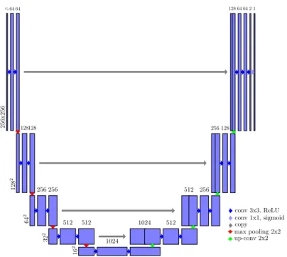
256x256 ci64 64 128 2 128128 64 2 256 256 32 2 512 512 16 2 1024 1024 512 512 256 256 128 128 64 64 2 1 conv 3x3, ReLU conv 1x1, sigmoid copy max pooling 2x2 up-conv 2x2
Figure 2: Schema of the neural network architecture
We used a network architecture similar to the one presented by Ronneberger et al.,11 U-Net. A schema of our architecture is included (figure 2).
The input of the original U-Net was 2D images, but we adapted it to accept a group of several adjacent slices. The network was trained to output the segmentation for the middle slice, based on the group of slices: it could use the surrounding slices as a context to help segment the middle slice. The volumes were then processed by groups of adjacent slices with a step of one slice, so that all slices are segmented. The dimensions of the input layer were256 × 256 × ci, whereciis the number of adjacent slices. We trained three networks withci∈ {1, 3, 7}
respectively.
2.3 Training
The cases were split into a training set (70% of the volumes) and a test set (the remaining 30%). The proportion of after-resection volumes versus during-resection volumes was the same in both sets.
The size of the volumes was bigger than the network input size: the volumes were between 300 and 500 voxels for each side. So the size of volumes had to be reduced to fit the network’s input size. For the training, we extracted one patch from each volume, so that the resection cavity is centered in the patch. First, a bounding box of the resection cavity was computed for all training volumes. Then, each bounding box was extended to the input size (256 voxels) such that the resection cavity is centered in the bounding box. Finally, slices or groups of adjacent slices were extracted from the bounding box.
Because of the dataset imbalance (around 95% of the voxels are background), we used a loss function based on the Dice score:12 loss(y
true, ypred) = 1 − Dice(ytrue, ypred). With the binary cross-entropy loss function, the
training did not converge easily: the network remained in a state where all the voxels were predicted background, because such predictions had a high score due to the dataset imbalance. Using a weighted binary cross-entropy loss with a higher weight for foreground voxels solved the convergence problem. However, it also increased the number of false positives, because the weight for background was lower so such errors were less penalized. The loss function based on the Dice score had neither the convergence nor the false positive problems, so we used this loss function.
(a) Downsampling method (b) Sliding window method (c) ROI method
Figure 3: Example prediction slice before thresholding
2.4 Testing
The test volumes also had to be reduced to the network’s input size. We tested three methods: (1) downsampling, (2) using a sliding window, and (3) estimating a bounding box with downsampled input and running the network again on that region at original scale (referred to as region-of-interest, or ROI, method). In the downsampling method, the input images were downsampled and the resulting prediction from the network was upsampled to the original size. In the sliding window approach, overlapping patches were extracted from the input images and the resulting prediction patches were averaged. The stride between consecutive patches was 64 so that each 256x256 patch had high overlap with neighboring patches. In the region of interest method, the network was first run on the downsampled images. Then, a 256x256x256 bounding box centered on the detected cavity was extracted from the original volume. The network was then run on that bounding box, in order to obtain a more precise prediction (at the original scale).
2.5 Post-processing
The output predictions were thresholded to get a binary mask. We used a threshold of 0.5 for the downsampling and ROI method, and 0.1 for the sliding window method. A lower threshold was used because the intensity on the edges was lower for the sliding window method. The patches containing only a part of the cavity tended to not detect the cavity, which lowered the final voxel value when the average value of all patches was taken. An example of this is given figure 3. In order to remove small and disconnected false positives around the cavity, only the biggest connected component was kept in the final result.
3. RESULTS
All the methods we tested were successful for most of the cases. With our best performing method (one context slice and ROI sampling), the Dice scores12 range from 0.68 to 0.96. Example predictions for each of the ten test
cases are presented figure5. Nine of the ten test cases were completely successful, with no obvious false areas and Dice scores above 0.75. The other case (case 8 after) had the most artifacts (noise and missing edges, see figure
1). It also had the highest inter-rater variability. The major part of the cavity was still correctly segmented, and the errors were located around the edges where the two observers also disagreed (see examples figure 6). As the network agreed with observer 2 in these areas, the Dice score for this case is substantially better when compared to observer 2’s segmentations: the score is 0.78 compared to observer 2 (whereas it is 0.68 compared to observer 1). Also in this case, the network successfully segmented the left part although a part of the white contour is missing (figure6b).
The mean Dice score for both inter-rater and intra-rater was 0.89. The Dice scores were over 0.9 for eight of the ten cases for intra-rater and for seven cases for inter-rater. The other two cases were also the cases were the automated method was less successful. With a mean Dice score of 0.86, the automated method achieves results that are comparable to manual segmentation. Figure7acompares the Dice scores of our best performing method with the inter- and intra-rater variability.
Figure7bshows the Dice scores12for each method. Each box correspond to a number of context slices, and contains the values for the three sampling methods.
In all contexts, the sliding window and ROI sampling methods had similar results. Results obtained with the downsized images were not as good as the sliding window and ROI methods. With the downsampling method, parts of the resection cavity were not detected in some slices. It is likely that the downsampling reduces the
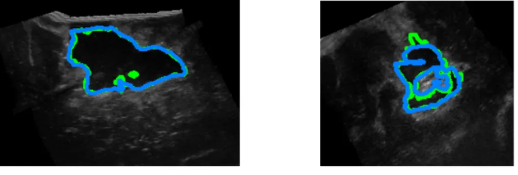
(a) A correct prediction (b) A correct prediction in a noisy image
Figure 4: Example results (green: ground truth, blue: prediction)
Case 2 after 4 after 8 after 17 during 19 after
Middle slice
Dice 0.90 0.83 0.68 0.93 0.95
Case 19 during 21 after 24 after 25 during 26 during
Middle slice
Dice 0.96 0.96 0.76 0.76 0.87
Figure 5: Per case results (green: ground truth, blue: prediction)
(a) Disagreement in the area without clear contours (b) Disagreement in the noisy area
dice 0.70 0.75 0.80 0.85 0.90 0.95
best−o1 best−o2 inter intra
● ● ● ● ● ●
best-o1: best method compared to observer 1 best-o2: best method compared to observer 2 inter: observer 1 compared to observer 2 intra: observer 1 variability
(a) Best method (ROI sampling, ci= 1) compared to
intra- and inter-rater variability
dice 0.0 0.2 0.4 0.6 0.8 1.0 DS SW ROI ● ● ● ● ● ci=1 DS SW ROI ● ● ● ● ● ci=7
DS: downsampling; SW: sliding window
(b) Comparison of sampling methods and number of context slices
Figure 7: Results Dice scores
neural network’s ability to recognize the textures representative of the resection. In two cases where the resection cavity was small, the network failed to detect the cavity and a bigger area was selected in the post-processing step. The downsampling step made the resection cavity even smaller, and was likely the reason why the network failed to detect the cavity. The two failing cases are shown as outliers in figure 7b. The sliding window method had a longer runtime because several patches were processed (about one minute per case on average, compared to 15 seconds for the downsampling and ROI methods). However it may be more reliable than the ROI method, which depends on the downsampling method providing a correct localisation of the cavity. This is difficult to evaluate precisely because our testing set contained only ten cases. For these ten cases, the localisation of the cavity provided by the downsampling method was accurate enough so the ROI method succeeded. Thus, while the sliding window and ROI approach had similar results, one or the other may be preferred depending on runtime and reliability constraints.
The results with more slices of context were similar to the ones with one slice of context: there were no visible improvement in the difficult areas with more slices of context. Seven slices of context is probably not enough context to make significant improvements. A 3D version of the neural network, using 3D convolutions and accepting 3D patches as input may have better results and will be explored in future work.
The mean runtime to run the network on one case was 15 seconds (for the downsampling and ROI methods), which is compatible with surgical procedures. In particular, the automated segmentation method can be used in model-based registration to take into account the resection cavity.
4. CONCLUSIONS
We created a ground truth dataset for segmentation of the resection cavity on the RESECT dataset. The artificial neural network we trained was successful in all the test cases. The obtained segmentations were highly accurate, with a mean Dice score of 0.86. In future work, we will evaluate the use of the segmented resection region for model-based registration of the pre-operative MR to intra-operative US images, which would enable improving image-guided tumor resection procedures.
ACKNOWLEDGMENTS
This work was partly supported by the French National Research Agency (ANR) through the framework In-vestissements d’Avenir (ANR-11-LABX-0004, ANR-15-IDEX-02).
REFERENCES
[1] Morin, F., Courtecuisse, H., Reinertsen, I., Lann, F. L., Palombi, O., Payan, Y., and Chabanas, M., “Brain-shift compensation using intraoperative ultrasound and constraint-based biomechanical simulation,” Medical Image Analysis 40, 133 – 153 (2017).
[2] Miga, M. I., Roberts, D. W., Kennedy, F. E., Platenik, L. A., Hartov, A., Lunn, K. E., and Paulsen, K. D., “Modeling of retraction and resection for intraoperative updating of images,” Neurosurgery 49(1), 75–85 (2001).
[3] Ferrant, M., Nabavi, A., Macq, B., Black, P. M., Jolesz, F. A., Kikinis, R., and Warfield, S. K., “Serial registration of intraoperative mr images of the brain,” Med Image Anal 6, 337–359 (Dec 2002).
[4] Bucki, M., Palombi, O., Bailet, M., and Payan, Y., [Doppler Ultrasound Driven Biomechanical Model of the Brain for Intraoperative Brain-Shift Compensation: A Proof of Concept in Clinical Conditions ], 135–165, Springer Berlin Heidelberg, Berlin, Heidelberg (2012).
[5] Fan, X., Roberts, D. W., Olson, J. D., Ji, S., Schaewe, T. J., Simon, D. A., and Paulsen, K. D., “Image updating for brain shift compensation during resection,” Operative Neurosurgery 14(4), 402–411 (2018). [6] Riva, M., Hennersperger, C., Milletari, F., Katouzian, A., Pessina, F., Gutierrez-Becker, B., Castellano, A.,
Navab, N., and Bello, L., “3d intra-operative ultrasound and mr image guidance: pursuing an ultrasound-based management of brainshift to enhance neuronavigation,” International Journal of Computer Assisted Radiology and Surgery 12, 1711–1725 (Oct 2017).
[7] Machado, I., Toews, M., Luo, J., Unadkat, P., Essayed, W., George, E., Teodoro, P., Carvalho, H., Martins, J., Golland, P., Pieper, S., Frisken, S., Golby, A., and Wells, W., “Non-rigid registration of 3d ultrasound for neurosurgery using automatic feature detection and matching,” International Journal of Computer Assisted Radiology and Surgery (Jun 2018).
[8] Xiao, Y., Fortin, M., Unsgård, G., Rivaz, H., and Reinertsen, I., “Resect: a clinical database of pre-operative mri and intra-operative ultrasound in low-grade glioma surgeries,” (2016).
[9] Noh, H., Hong, S., and Han, B., “Learning deconvolution network for semantic segmentation,” CoRR abs/1505.04366 (2015).
[10] Badrinarayanan, V., Kendall, A., and Cipolla, R., “Segnet: A deep convolutional encoder-decoder architec-ture for image segmentation,” CoRR abs/1511.00561 (2015).
[11] Ronneberger, O., Fischer, P., and Brox, T., “U-net: Convolutional networks for biomedical image segmen-tation,” CoRR abs/1505.04597 (2015).