A Comprehensive Probabilistic Framework to Learn
Air Data from Surface Pressure Measurements
The MIT Faculty has made this article openly available. Please share
how this access benefits you. Your story matters.
Citation
Ankur Srivastava and Andrew J. Meade, “A Comprehensive
Probabilistic Framework to Learn Air Data from Surface Pressure
Measurements,” International Journal of Aerospace Engineering,
vol. 2015, Article ID 183712, 19 pages, 2015.
As Published
http://dx.doi.org/10.1155/2015/183712
Publisher
Hindawi Publishing Corporation
Version
Final published version
Citable link
http://hdl.handle.net/1721.1/99151
Terms of Use
Creative Commons Attribution
A Comprehensive Probabilistic Framework to
Learn Air Data from Surface Pressure Measurements
Ankur Srivastava
1and Andrew J. Meade
21Massachusetts Institute of Technology, Cambridge, MA 02139, USA 2Rice University, Houston, TX 77005, USA
Correspondence should be addressed to Ankur Srivastava; [email protected] Received 11 May 2015; Revised 13 August 2015; Accepted 23 August 2015
Academic Editor: Christopher J. Damaren
Copyright © 2015 A. Srivastava and A. J. Meade. This is an open access article distributed under the Creative Commons Attribution License, which permits unrestricted use, distribution, and reproduction in any medium, provided the original work is properly cited. Use of probabilistic techniques has been demonstrated to learn air data parameters from surface pressure measurements. Integration of numerical models with wind tunnel data and sequential experiment design of wind tunnel runs has been demonstrated in the calibration of a flush air data sensing anemometer system. Development and implementation of a metamodeling method, Sequential Function Approximation (SFA), are presented which lies at the core of the discussed probabilistic framework. SFA is presented as a tool capable of nonlinear statistical inference, uncertainty reduction by fusion of data with physical models of variable fidelity, and sequential experiment design. This work presents the development and application of these tools in the calibration of FADS for a Runway Assisted Landing Site (RALS) control tower. However, the multidisciplinary nature of this work is general in nature and is potentially applicable to a variety of mechanical and aerospace engineering problems.
1. Introduction
INTRUSIVE aircraft anemometer booms have long been successfully used to measure air data parameters for subsonic and supersonic flight. Rapid development in aerospace and naval technology has continuously demanded smaller, less intrusive, and more accurate air data systems. Accuracy of probe based air data systems suffers at high angles of attack or when dynamic maneuvering is required. These same conditions can lead to degraded flying handling qualities [1]. Errors due to vibration, poor alignment, and physical damage during operation or maintenance can also pose significant limitations on the use of protruding booms. Probe based air data systems cannot be used with stealthy aircrafts because they increase the total radar cross-section of the body which can potentially jeopardize the mission and risk human lives. Hypersonic flight regimes are another area where probe based air data systems cannot be used because the vehicle nose reaches extremely high temperatures that might melt the protruding boom. Also, such flow protruding booms cannot be used with research aircrafts without disturbing the airflow or the boundary layer. Finally, air data booms are too heavy and costly to use with unmanned micro air
vehicles (MAVs) [2]. Reference [2] mentions that an 80% decrease in instrumentation weight and a 97% decrease in instrumentation cost can be gained by eliminating probe based air data systems from MAVs.
In order to overcome the above mentioned drawbacks, flush air data sensing (FADS) systems were developed. A pop-ular flush air data system is a series of pressure taps mounted on a vehicle periphery that can be used to derive airflow parameters. FADS systems were first developed during the X-15 program. A hemispherical nose with pressure sensors was installed on this hypersonic aircraft to measure stagnation pressure and wind direction during reentry [3]. Further research on FADS for hypersonic vehicles was conducted during the Space Shuttle program [4]. After enjoying success on hypersonic flights the compatibility of FADS was tested on supersonic and subsonic flight regimes. The authors of [5] developed and flight-tested a flush air data sensing system for the F-18 Systems Research Aircraft (Figures 1 and 2). The authors concluded that the developed nonintrusive technique was clearly superior to the probe based air data systems. They showed that FADS were unaffected by dynamic flight maneuvers and they performed well in high angle of attack flights. FADS systems are also unaffected by vibration and
Figure 1: Flush air data system installation at the nose of the F-18 Systems Research Aircraft [1].
Figure 2: FADS Ports on Space Shuttle Columbia and F-18 [21].
icing effects and are less prone to damage during operation and maintenance. They are an ideal choice for stealth vessels because they are self-sustained and give no additional radar cross-sectional area to the vessel signature.
Other nonintrusive air data systems include flush mount-ed optical air data systems and flush mountmount-ed heat films. The optical air data systems transmit lasers or acoustic signals generated by electromechanical transducers or loud speakers through a fluid medium to one or multiple receivers and measure the travel time to infer air data information. Even though these systems are nonintrusive, they are not self-sustained and are expensive and heavy to use [6].
1.1. Challenges in Estimating Air Data of a Flush Air Data Sens-ing System. As previously mentioned, FADS systems infer the
air data parameters from pressure measurements taken with an array of ports that are flush to the surface of the aircraft. However, because the locations of the pressure measurements are on the outer surface of the aircraft on geometrically simple components (e.g., hemispherical or conical nose), properties of the local flow fields like compressibility and flow separation can drastically affect these devices. Unlike aircraft, the FADS for bluff bodies like buildings must be placed
y x 𝜃 𝛽 P(𝜃) V∞
Figure 3: Two-dimensional flow about a right circular cylinder.
completely around the structure and can routinely experience separated and unsteady cross-flow. Finally, to compete with conventional air data systems, the FADS must be able to estimate wind speeds (𝑉∞) over a range of 40 to 120 fps, ±3.4 fps (i.e., ±2 knots), and wind directions (𝛽) ranging from 0 to 360 degrees,±2 degrees. For more details on assessment of conventional air data systems please refer to [7].
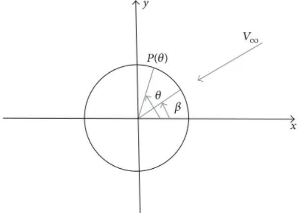
Using the incompressible flow about a right circular cylinder as an example of a bluff body (Figure 3), the problem of estimating relative wind speed and direction from the surface pressure at position 𝜃 can be framed as either a forward or inverse mapping problem. That is,
the forward problem
𝑃 = 𝐹 (𝜌∞, 𝑉∞, 𝜃, 𝛽) ; (1) the inverse problem
𝑉∞= 𝐺 (𝑃, 𝜌∞, 𝜃, 𝛽) ,
𝛽 = 𝐺 (𝑃, 𝜌∞, 𝑉∞, 𝜃) . (2) For simple geometries, closed-form semiempirical equations can be developed and used to solve the forward prob-lem of estimating the pressure coefficient, 𝐶𝑝, given the freestream wind speed and direction [8]. Panel methods [9] and other popular computational fluid dynamic (CFD) based approaches solve the forward problem on more complex geometries given the freestream wind speed and direction. However, this approach requires guessing the freestream velocity and solving for the pressure distribution until it matches the measured values. To solve the inverse problem, look-up tables from experimental fluid dynamics (EFD) can be constructed for the mapping function𝐺. Unfortunately, look-up tables suffer from a number of drawbacks when their real-time use is considered including the inability to handle high-dimensional inputs, noisy data, and nonlinear interpolation. It is proposed that machine learning methods, specifically Artificial Neural Networks (ANNs), be explored to solve the inverse problem. In addition, this paper will demonstrate how a particular form of ANN can also be used to determine the best locations for sensor placement,
to maximize available FADS data by seamlessly combin-ing CFD and EFD outputs, and to help guide physical experiments thereby minimizing the time needed in testing facilities.
1.2. Intersection of Statistical Learning and Fluid Dynamics.
In general, mechanical and aerospace engineering systems present a number of challenging problems especially in the field of fluid dynamics. Understanding pressure and velocity distributions of the fluid flow is essential to the design and control of complex multicomponent interacting systems. Experimental and computational methods in fluid dynamics have long been successfully used to model such engineering systems. However, intensive research in both fields spanning over several decades has highlighted several shortcomings [10]. Over the last few decades, as complexity of engineering systems increased, it became a necessity rather than academic curiosity to adopt interdisciplinary approaches to study a system. Intelligent data understanding tools like Artificial Neural Networks (ANNs) [11] and kernel methods from machine learning and statistics have enjoyed increased pop-ularity in mechanical and aerospace engineering problems. However, the following issues remain.
1.2.1. Formalization of the Final Network. A typical 3-layer
ANN involves several parameters to be defined by the user including (a) number of neurons in the hidden layer, (b) initial weight matrix, (c) parameters of the basis function, and (d) values of the learning rates. Ad hoc procedures exist for choosing each of these parameters. However, lack of a principled approach to network construction generally leads to an overparameterized network. To optimize the structure of the network exhaustive grid search or cross-validation approaches are often needed. To attack this problem we focus on greedy scattered data approximation approaches [12]. In these approaches the user needs to load only the training and test sets and the algorithm solves for the required parameters in a self-adaptive greedy fashion. In other words, greedy scattered data approximation approaches provide a formal way to construct networks in an optimized manner.
1.2.2. Choice of Training Data. It is often unclear how many
training points would be sufficient for an acceptable general-ization error and how these training data should be chosen. Traditionally, network training and testing is done only after all the data is collected. This is called passive learning in the machine learning literature, where the learning algorithm does not take part in the data collection procedure. Collecting data without taking into account the input-output functional relationship like the traditional Latin Hypercube Design [13] methods can result in choice of data that add little to no information to training of the network and can even hurt the generalization ability of the training method. This is especially a problem when data collection is costly, like flight tests or when the input domain is excessively large to sample. Active learning [14] methods are popular in the machine learning literature where the learning algorithm takes part in the data collection procedure and new input configurations
Pressure sensor
(a) (b)
Figure 4: (a) Wind tunnel model of the RALS tower [7] and (b) actual image of the RALS tower.
are sampled such that they maximize some information gain criterion in a principled manner. These sampling procedures are essentially sequential in nature and not only help the engineers to accelerate through the test matrix, but also allow the learning algorithm to have better generalization capability.
1.2.3. Data-Model Fusion: Fusing Sparse High Fidelity Wind Tunnel Data with Low Fidelity CFD Trends. ANNs provide
a powerful tool to interpolate and extrapolate experimental data. However, it is beneficial to have a framework that can integrate experimental data with models of variable fidelity. Regularization approaches provide us with such a framework where it is possible to include physical knowledge of the system in the form of numerical simulations to be included as a priori information in the training of the network [15]. Such a data assimilation procedure can be seen as approximating noisy and scattered experimental data with physics based smoothness. It can also look as improving low fidelity numerical simulations with more accurate experimental data. This tool can result in acceptable flow field solutions by fusing fewer experimental data with possibly lower fidelity CFD data thereby saving precious resources.
For the purpose of solving the inverse problem of FADS calibration discussed in Section 1 and similar engineering problems, a multidimensional learning tool should address the hyperparameter selection problem previously mentioned, operate as easily on high-dimensional data as it does on low-dimensional ones, and provide the user with an assurance that the tool will give its best performance on an unseen test set. The tool should also require a minimum of storage and require as little user interaction as possible. To this end, we use Sequential Function Approximation (SFA), an adaptive tool, developed earlier for solving regression and classification problems [16] with little user interaction to determine hyperparameters.
The first objective in this work is to develop a computa-tional surrogate that can predict wind speed and yaw angle from surface pressure measurements. The surrogate should not have wind speed prediction errors greater than±3.4 fps and yaw angle prediction errors greater than±2 degrees. The second objective is to investigate how data-model fusion can help to better represent the coefficient of pressure distribution across the bluff body surface. The third objective is to develop a general intelligent sampling strategy with active learning and SFA on regression problems.
Section 2 discusses estimation of air data parame-ters from surface pressure measurements in more detail. Section 2.2 presents freestream wind speed and direction estimation techniques and the results on the current problem. Section 3 briefly discusses the role of regularization tech-niques in fusing wind tunnel data with numerical models of variable fidelity. Section 4 begins by introducing the fields of active learning and optimum experiment design. Sections 4.1 and 4.2 discuss a G-optimal design procedure with SFA and present its implementation issues application on a simulated regression problem. Finally, Section 4.3 presents the application of this technique on the FADS problem.
2. Freestream Wind Speed and
Direction Estimation
The Runway Arrested Landing Site (RALS) control tower is located at the Naval Air Warfare Center Lakehurst, New Jersey. Wind tunnel tests were conducted on a 1/72 scale model of the RALS control tower [7]. One pressure sensor was mounted on each face of the control tower as shown in Figure 4. A four-hole Cobra probe was used to measure the freestream wind speed and direction. The FADS system was tested on a variety of wind speeds ranging from 40 fps to 120 fps approaching the model from all 360 degrees of yaw. Variation of the wind incidence in three dimensions will be a
South face port West face port
North face port East face port
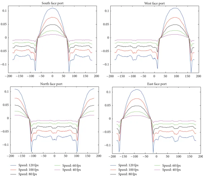
0.1 0.05 0 −0.05 −0.1 0.1 0.05 0 −0.05 −0.1 0.1 0.05 0 −0.05 −0.1 0.1 0.05 0 −0.05 −0.1 −200 −150 −100 −50 0 50 100 150 200 −200 −150 −100 −50 0 50 100 150 200 −200 −150 −100 −50 0 50 100 150 200 −200 −150 −100 −50 0 50 100 150 200 Speed:120 fps Speed:100 fps Speed:80 fps Speed:60 fps Speed:40 fps Speed:120 fps Speed:100 fps Speed:80 fps Speed:60 fps Speed:40 fps
Figure 5: Surface pressure (psi) variation versus the yaw angle for different wind speeds.
part of the future work. In addition, the scope of this work is to develop a computational framework to predict wind speed and direction from pressure measurements and not to conduct the wind tunnel experiments. The experimental setup is mentioned here briefly for completeness.
Borrowing from flight mechanics literature and restrict-ing our problem to two dimensions,𝛽 is defined as the yaw angle and is measured in the anticlockwise sense with respect to the centerline of the model. So winds approaching the south port have𝛽 = 0 degrees, for the east port 𝛽 = 90 degrees, for north port𝛽 = 180 degrees, and for the west port 𝛽 = 270 degrees. In Figure 5 shown surface pressure is plotted for each pressure port. The pressure port on the south face bears positive pressure values when wind is incident head-on at the pressure port and bears negative values for winds hitting the north face. Similarly the pressure port on the west face bears positive pressure values when the yaw angle is positive and bears negative values for negative yaw values. Also evident from Figure 5 is that the pressure ports do not show much variation when they are on the leeward side.
2.1. Forward and Inverse Problems. Computational
algo-rithms like neural networks that learn from data can be very effective in solving inverse problems and bear potential advantages in the construction of the FADS mapping func-tion 𝐺 (Section 1.1) compared to look-up tables. Examples of neural networks advantages include high-dimensional mapping, smoother nonlinear control, intelligent empirical learning, and fewer memory requirements [17–20]. For speed of evaluation, reduced complexity, and the potential for graceful performance degradation with the failure of pressure sensors, the inverse problem is solved using only two sets of neural networks with pressures read from all surface sensors,
𝑞 = 𝐺1 (𝑃1, . . . , 𝑃𝑑) ,
𝛽 = 𝐺2 (𝑃1, . . . , 𝑃𝑑, 𝑉∞) . (3)
2.1.1. Dynamic Pressure. Even though our problem involves
turbulence and cross-flow about nontrivial geometries, the existence of a functional relationship between𝑃 and 𝑉∞and
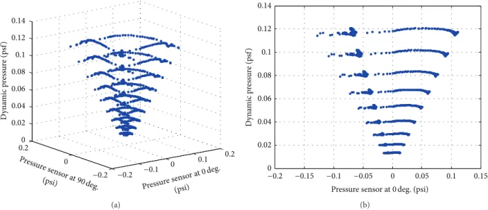
(a) 0 0.02 0.04 0.06 0.08 0.1 0.12 0.14 −0.2 −0.15 −0.1 −0.05 0 0.05 0.1 0.15 D yna mic p res sur e (psf )
Pressure sensor at0 deg. (psi)
(b)
Figure 6: Dynamic pressure hypercone represented as a function of (a) two pressure sensors and (b) one pressure sensor.
between𝐶𝑝and𝛽 can be safely assumed. The wind speed was predicted using only the surface pressure data while the wind direction was predicted using the pressure coefficient data derived from measured pressure and predicted wind speed values. It is noted that this coupling of networks put the bur-den of high accuracy on the wind speed predictor. Freestream air density was kept constant in the current problem which makes prediction of freestream wind speed equivalent to dynamic pressure. Sequential Function Approximation was used to construct one RBF network to model 𝐺1 and the corresponding wind speed surrogate is represented by
𝑞pre= 𝑛 ∑ 𝑖=1
𝑐𝑖exp(ln [𝜆𝑖] ∗ ( ⃗𝑝test− ⃗𝑝∗𝑖) ⋅ ( ⃗𝑝test− ⃗𝑝∗𝑖)) + 𝑏𝑖.
(4)
The hypersurface for the current dynamic pressure prediction problem can be imagined as a hypercone with surface pressure as input dimensions and dynamic pressure as output. Dynamic pressure increases linearly with surface pressure given a yaw angle𝛽 for all pressure sensor positions, 𝜃. So each wind tunnel sweep at a constant speed would yield data points lying at the contours of the hypercone. Also, the slope of the hypercone corresponds to the coefficient of pressure at a given value of the yaw angle𝛽.
Figures 6(a) and 6(b) show the aforementioned hyper-cone in two and one dimension, respectively. Looking at Figure 6(b), it is evident that the span of the cone includes all pressure measurements of the sensor at𝜃 = 0 degrees at all wind speeds and yaw angles. The right edge of the cone corresponds to the case when the sensor faces directly the wind or𝛽 = 𝜃. As one moves from the right to the left edge of the cone the separation at the pressure sensor increases. A RBF network constructed by SFA can suitably approximate this hypercone; however it is possible that a better approach might exist for this approximation. This will constitute a part of the future work.
Coefficient of pressure −1.5 −1 −0.5 0 0.5 1 200 150 100 50 0 −50 −100 −150 −200 Ya w a n gl e
Figure 7: Nonuniqueness of the yaw angle prediction problem at 120 fps with one pressure sensor.
2.1.2. Wind Direction. Once the wind speed predictor was
available, the test surface pressure values were divided by the corresponding predicted dynamic pressure to obtain the test coefficient of pressure values. Several ways exist to predict the yaw angle𝛽. One straightforward way is to construct one RBF network for𝐺2 given by (5), where
𝛽pre=∑𝑛
𝑖=1
𝑐𝑖exp(ln [𝜆𝑖] ∗ ( ⃗𝑐𝑝,test− ⃗𝑐𝑝,𝑖∗) ⋅ ( ⃗𝑐𝑝,test− ⃗𝑐𝑝,𝑖∗ )) + 𝑏𝑖.
(5)
However, unlike dynamic pressure, yaw angle prediction is a strongly nonunique problem.
Figure 7 shows the variation of the yaw angle with bow side coefficient of pressure at 120 fps. It is evident from Figure 7 that at least two solutions for𝛽 exist for most values
of𝐶𝑝, and except when the pressure sensor faces separated flow. Here it is important to elaborate on the meaning of nonuniqueness when learning yaw angle as a function of pressure measurements. If we try to fit a metamodel for yaw angle as a function of coefficient of pressure, then from Figure 7 we realize that, for any given coefficient of pressure, say zero, there are at least two possible yaw angles that can yield coefficient of pressure of value zero on the wall. Similarly for a coefficient of pressure value of −0.5, there are more than 2 values of yaw angles that can result in coefficient of pressure of value−0.5. Since building metamodels for yaw angle as a function of coefficient of pressure is nonunique we try to build metamodels for the forward problem as described below. It is important to mention here that as we add more sensors the problem becomes less nonunique and we have more information to predict the yaw angle. In this problem four sensors are not enough to build accurate metamodels as shown in (5), motivating development of method shown below. It will be a very interesting problem to determine the minimum number of sensors and their location to maximize prediction accuracy and will constitute part of future work. A simple forward problem approach was developed to estimate the yaw angle which is discussed next.
In this approach, the forward problem of approximating 𝐶𝑝 as a function of the yaw angle𝛽 is addressed. It is well known from fluid mechanics that in external flow 𝐶𝑝 is a function of both𝛽 and the surface pressure sensor position, 𝜃. Constructing a surrogate model of 𝐶𝑝as a function of both 𝛽 and 𝜃 is equivalent to approximating 𝐶𝑝for each pressure sensor as a function of just the yaw angle𝛽. Even though this increases the memory requirements, it yields faster and more accurate models for𝐶𝑝. Once a network has been constructed to represent each sensor, the objective function in (6) can be minimized to predict the yaw angle for a vector of test pressure coefficients: 𝛽pre= min 𝛽 𝑁𝑆 ∑ 𝑖=1 (𝑝test(𝑖) 𝑞pre − 𝑐𝑝,𝑖(𝛽)) 2 . (6) Here𝑁𝑆 is the number of pressure sensors, 𝑐𝑝,𝑖represents the approximated𝐶𝑝for the ith pressure sensor,𝑝testis the test vector of pressure values, and 𝑞preis the predicted dynamic pressure for𝑝test. It should be noted here that to predict wind direction, the predicted dynamic pressure is used and not the preknown dynamic pressure. A simple line search for𝛽 would suffice for the above minimization problem. However, searching for𝛽 over the entire range of [−180, 180] degrees would be wasteful, so𝛽 could be searched over [𝛿 − 𝜀, 𝛿 + 𝜀], where 𝛿 is the pressure sensor position that bears the maximum surface pressure value and𝜀 is a value of the yaw angle chosen by the user so that range for the line search is sufficiently large. Because𝐿2 norm is the most resilient to random noise it was chosen to express the differences between the test𝐶𝑝 and predicted𝐶𝑝. Also, (6) allows the user to put weights on the contribution of each pressure sensor. Different weights could be helpful in situations where there is a combination of high and low fidelity sensors, or in the case of sensor damage or local flow field disturbance.
Besides ease of learning and better redundancy to noise this wind direction estimation approach uses all the available sensors for prediction instead of just those in a quadrant. The above mentioned algorithms have also been tested for a surface vessel and experimentally verified at the Fluid Mechanics Lab at the NASA Ames Research Center [16, 21]. Besides learning the air data parameters, this work extends to sequential experiment design and data-model fusion for the current problem.
2.2. Results. In this section wind speed and direction
esti-mation accuracies are presented. Results for the RALS tower problem are presented using the estimation approaches discussed above. The SFA algorithm was implemented using the MATLAB programming environment on a Windows-configured PC with a Pentium 4 2.66 GHz processor and 1.0 GB of RAM.
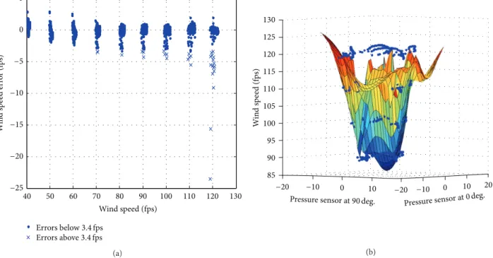
Wind tunnel data for the RALS tower was available at speeds ranging from 40 fps to 120 fps as wind direction was varied from−180 to +180 degrees at increments of 2 degrees. All available data points were used in the test set, while a training set was created by taking data present at increments of 4 degrees at each wind speed. It should be noted here that, by this choice of training data, it consists only about half of the number of points in the test set. Once the training and test sets were constructed one network was constructed to predict dynamic pressure according to (4). The tolerance parameter was kept close to zero at a value of1𝑒 − 6 so as to minimize any errors in the approximation of 𝐶𝑝. Figure 8(a) shows the prediction errors if SFA was used to construct one RBF network for wind speed prediction as a function of surface pressure. However, there are several errors larger than the tolerance of 3.4 fps at 120 fps and on a closer look one realizes that most of the errors occur at yaw angles in the vicinity of 0, 90, 180, and−90 degrees. One possible explanation for the wind speed errors displaying a bias at the highest wind speed is shown in Figure 8(b). In this problem, a hypercone is approximated with radial basis functions (RBFs). RBFs model the smooth slopes of the hypercone; however they do not approximate the flat top of the hypercone that exists due to the wind speeds of the highest magnitude.
Next we present a heuristic which could be used to reduce the errors shown in Figure 9(a). As mentioned before most of the errors occur in the vicinity of the 0, 90, 180, and−90 degrees. For the following ranges of the yaw angle|𝛽| ≤ 25∘, |𝛽−90∘| ≤ 25∘,|𝛽| ≥ 155∘, and|𝛽+90∘| ≤ 25∘, the correspond-ing pressure sensors face a head-on freestream wind and bear a positive pressure value and the remaining sensors bear a negative pressure value. This a priori information was used in conjunction with the dynamic pressure model to improve prediction in the following manner. Training points lying in the above mentioned range were set aside before starting to construct (4). During testing, if a test point is such that only one sensor bears positive pressure value, the dynamic pressure of that test point was predicted using a simple nearest neighbor search from the training points that were set aside. Prediction of dynamic pressure is coupled with coefficient of pressure or the yaw angle. If𝛽 of a test point is known a priori, linear dependence of dynamic pressure with surface pressure
(a) (b)
Figure 8: (a) Wind speed prediction on RALS tower data using just one network for wind speed given by (4). (b) Example surrogate of the wind speed hypercone in 2 dimensions.
0 100 200 300 400 500 600 700 800 900
Number of basis functions 2 0 −2 −4 −6 −8 −10 L oga ri thm o f dis cr et e inner p ro d uc t o f re sid ua l er ro r (a) WOD speed (fps) 1.5 1 0.5 0 −0.5 −1 −1.5 −2 50 40 60 70 80 90 100 110 120 130 Errors below3.4 fps W O D sp eed er ro r (f ps) (b)
Figure 9: (a) Logarithm of discrete inner product norm of residual error. (b) Wind speed prediction errors on the RALS tower data when training was conducted on data at every 4-degree increments of yaw angle.
is easily used to predict the dynamic pressure of a test point. With the help of this heuristic one can approximately deduce 𝛽 and use linear dependence of dynamic and static pressure to predict dynamic pressure and thereby wind speed of a test point.
Figures 9(a) and 9(b) show convergence of residual error and wind speed prediction errors on the test set, respectively. Blue dots show errors below the acceptable error tolerance of
3.4 fps. The maximum error of 25 fps shown in Figure 8(a) was reduced to less than 2 fps with the help of the nearest neighbor heuristic.
Once the wind speed predictor was in place, the predicted dynamic pressure values were used to obtain test coefficient of pressure values. The resulting test𝐶𝑝values were then input to the forward approach discussed in the previous section. To implement the forward problem approach first four models
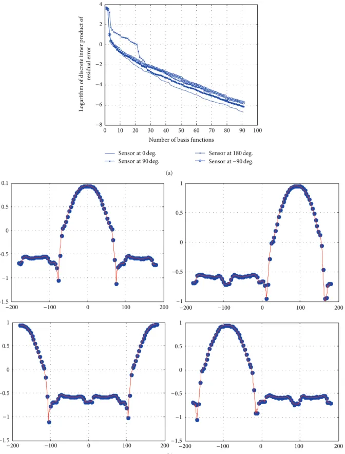
of pressure coefficient were constructed as a function of the yaw angle. Figures 10(a) and 10(b) show the residual error convergence and approximation of𝐶𝑝for each pressure sensor, respectively. Since sufficient noise-free training data was available, tolerance was kept low and so the𝐶𝑝 models interpolate the wind tunnel data accurately.
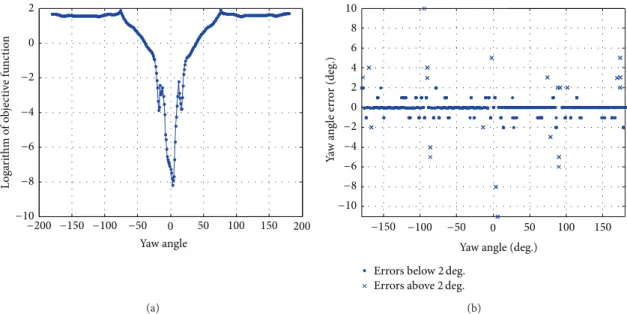
Ability of SFA to handle noise and sparsity in training data will be covered in future work. Once the𝐶𝑝models have been constructed the objective function shown in (6) was minimized by a line search to predict the yaw angle for each test point. Figure 11(a) shows an example of the logarithm of the objective function for a test point with a yaw angle of zero degrees.
Figure 11(b) shows yaw angle prediction errors on the RALS tower data using the forward problem approach.
3. Data-Model Fusion: Global Scaling via
Surrogate Modeling
Estimating freestream wind speed and direction from surface pressure measurements is an posed problem. The ill-posedness is induced due to the nonuniqueness of the problem which is worsened in the presence of noise in the pressure data. The inverse problem addressed in this paper is to reconstruct a complete pressure signal given sparse, noisy, and incomplete experimental data. This work develops an alternate method of fusing experimental and computational data to approximate pressure signals to estimate freestream wind speed and direction. The approach uses SFA as the inverse modeling tool and applies a simplified Tikhonov-related regularization scheme to correct for the original data error. The purpose of this section is to introduce a fusing approach using SFA that maximizes the use of experimental data with the help of CFD data in approximating a smooth, continuous, and accurate pressure distribution. The fusing approach first involves calculating the error function of the CFD and experimental data defined by the following equation:
𝑒 (𝜉𝑖) = 𝑢CFD(𝜉𝑖) − 𝑢EXP(𝜉𝑖) , (7) for𝑖 = 1, . . . , 𝑠, where 𝑠 is the number of training data sets. The error vector, 𝑒, is then used to train the SFA network to a predetermined tolerance,𝜏. The resulting error surface, 𝑒(𝜉), will naturally involve some scatter directly related to the experimental data noise. Training the network to the given tolerance allows the SFA to regulate the noisy experimental data with a priori CFD information. Assuming the 𝑢CFD surface is known, then the error surface approximation, 𝑒SFA, can be subtracted from the 𝑢CFD(𝜉) data to give the approximation in
𝑢SFA= 𝑢CFD− 𝑒SFA. (8) The𝜏 value can be regarded as the regularization parameter and controls how well the approximations fit the experi-mental or CFD data. A very high tolerance value allows the training process to end prematurely with very few network units. As a result, the network “underlearns” the training data
and the majority of the approximations reach a value of zero. For data points with an error value of zero, (8) shows that the approximation value will reproduce the CFD data. On the other hand, a very small tolerance value will force the network to use too many network units to reach the smallest possible tolerance. In this case, the network “overlearns” the training data and will fit even the experimental noise in the error surface. As a result, the approximations will reproduce the experimental data. The user must carefully choose the tolerance value to best fit the experimental data using the CFD information based on the noise in the data. Similar approaches have been developed in [22–25].
In external flow past bluff bodies, coefficient of pressure is a function of the yaw angle 𝛽 and local pressure sensor position𝜃. In the RALS tower problem wind tunnel data is available at only four values of𝜃 = [−90, 0, 90, 180] degrees shown in Figure 12. A complete representation of 𝐶𝑝 as a function of 𝛽 and 𝜃 is necessary because it can possibly inform the experimentalist what locations should be chosen for pressure sensor installation to improve wind direction prediction accuracy.
Numerical solutions, however, provide full coefficient of pressure distribution as a function of yaw angle and pressure sensor position. The data-model fusion technique discussed here could similarly be applied to correct low fidelity 𝐶𝑝 solutions even at values of 𝜃 where no wind tunnel data is available. This could be done simply by calculating the differences between the wind tunnel and CFD solutions at 𝜃 = [−90, 0, 90, 180] degrees. Once the differences have been calculated, it can be treated as a function approximation problem by SFA with𝛽 and 𝜃 as inputs and 𝐶𝑝 as output. Once a surrogate to the hypersurface of differences has been created, it could be added to the CFD𝐶𝑝surface to obtain a 𝐶𝑝distribution shown in Figure 13. The numerical solutions were extracted at 56 values of𝜃 for each yaw angle.
4. Sequential Experiment Design
In the previous sections, passive learning techniques were discussed for the FADS problem, where a learning algorithm, like SFA, acts only after the training data set has been collected. The learning algorithm does not take part in the data collection procedure. Traditionally, popular space filling experiment design strategies like Latin hypercube sampling (LHS) are used to plan the data collection procedure. Use of LHS is popular with Monte Carlo techniques to estimate uncertainty in computer models. It has been proven that fewer samples are required with LHS compared to random sampling when estimating the output with a given variance [13]. Latin hypercube sampling is a simple and effective space filling sampling technique which does not need or assume the input-output functional relationship. Even though LHS is better than random sampling, a significant improvement is possible if the functional form of the input-output rela-tionship is assumed and data are sampled from those regions where the output variance of the assumed input-output func-tion is maximum. It is thought that advances in experiment design strategies will not only benefit the training of FADS but the fields of EFD and CFD in general. Suboptimal designs
0 10 20 30 40 50 60 70 80 90 100 Number of basis functions
4 2 0 −2 −4 −6 −8 L oga ri thm o f dis cr et e inner p ro d uc t o f re sid ua l er ro r Sensor at0 deg. Sensor at90 deg. Sensor at180 deg. Sensor at−90 deg. (a) 0.1 0.5 0 −0.5 −1 −1.5 −200 −100 0 100 200 −200 −100 0 100 200 1 0.5 0 −0.5 −1 −200 −100 0 100 200 1 0.5 0 −0.5 −1 −1.5 1 0.5 0 −0.5 −1 −1.5 −200 −100 0 100 200 (b)
Figure 10: (a) Residual error convergence and (b)𝐶𝑝prediction by a model of each pressure sensor. Blue dots represent wind tunnel data and the red line represents approximation by SFA as a function of the yaw angle. Clockwise from top plots shows𝐶𝑝model of pressure sensor at 0, 90,−90, and 180 degrees.
Yaw angle 2 0 −2 −4 −6 −8 −10 −200 −150 −100 −50 0 50 100 150 200 Lo ga ri th m o f o b jecti ve fu n cti o n (a) (b)
Figure 11: (a) Logarithm of objective function of (6) obtained after a line search conducted for a test point with a yaw angle of 0 degrees. (b) Yaw angle prediction errors on the RALS tower data when training was conducted on data at every 4-degree increments of yaw angle using the forward approach.
Figure 12: Wind tunnel coefficient of pressure as a function of yaw angle and pressure sensor position.
could be a serious problem if the input domain is excessively large or output determination is expensive. Careful selection of training points is also important to construct surrogates with low generalization error. Input sampling strategies where the learning algorithm actively takes part in the data collection procedure are studied in the field of active learning or query learning as suggested by its name. In statistics they are studied in the field of Optimal Experiment Design (OED) [26].
4.1. Active Learning for Regression Problems. For continuous
valued problems, significant research has been done in the field of statistics under the name of Optimal Experiment Design [26]. An acceptable active learning method for regres-sion problems should be able to minimize mean squared error
0 100 200 0 100 200 Pressure position angle Yaw a ngle 2 1 0 −1 −2 −3 −200 −200 −100 −100 C o efficien t o f p ressur e
Figure 13: Fused coefficient of pressure surface as a function of yaw angle and pressure sensor position.
more than the passive learning methods using fewer training points. Consider a general regression problem in
𝑦 (𝑥) = 𝑓 (𝑥, 𝛽) + 𝜀 (9) with 𝑑 dimensional inputs 𝑥 ∈ R𝑑, output 𝑦 ∈ R, and random errors𝜀 which we assume to be independent and uncorrelated. Given a small, finite number of training samples𝑠, the parameters of this regression problem can be estimated that minimize the mean squared error given by
𝐸MSE= ∫ 𝑓(𝑥, 𝛽) − 𝑓(𝑥)2𝑑𝑄 (𝑥) , (10) where𝑄 is the environmental probability. However, since the environment is generally realized by the user only via the
𝑠 number of training points, the following estimated mean squared error in (11) is minimized to estimate the parameters 𝛽: 𝑆 ( 𝛽) = min 𝛽 1 𝑠 𝑠 ∑ 𝑖=1(𝑓 (𝑥𝑖, 𝛽) − 𝑦 (𝑥𝑖)) 2 . (11) Given a finite number of training samples and a learning algorithm to estimate the parameters 𝛽, an optimum active learning scheme would compute a sample point where the expected mean squared error over the whole input domain is maximum. Estimation of the future generalization error could be a very computationally demanding task for both pool based and population based active learning methods where information about the conditional probability dis-tribution is either known or assumed. Kindermann et al. [27] use a Bayesian theoretic framework to develop an active learning method where they use Markov Chain Monte Carlo methods to approximate the expected loss. Roy and Mccallum [28] estimate the expected error by adding all possible labels for each unlabeled sample to the training set. The proposed brute force approach is infeasible for regression problems and classification problems with many classes. The authors propose several ways to make this procedure efficient, for example, use of Na¨ıve Bayes and SVMs where addition of a new training point does not need retraining, or estimate EMSE only on the neighborhood of the candidate points which compromises the generality of the approach. It is important to note here that methods such as Krig-ing/Gaussian Processes have the Expected Improvement cri-teria which can be used for adaptive sampling and estimating uncertainty in results. However, the authors wanted to show that a similar framework can be developed with other state-of-the-art metamodels. In the current FADS application, the number of training data points is high which would take longer for the Gaussian process or Kriging models to train. The SFA method trains quickly while preserving accuracy of the solution. And we show that with this new method we can also construct a framework for adaptive sampling and fusing high and low fidelity data.
Since estimation of expected future loss is infeasible, one can rely on the bias-variance decomposition of EMSE to estimate a sample where the expected error would be maximum. For a given sample 𝑥, let 𝑦 = 𝑓(𝑥, 𝛽), 𝑦 = 𝑓(𝑥, 𝛽), and 𝑦 = 𝐸[ 𝑦] be the true output, estimated output, and the expected value of the estimated output, respectively. The expected value can be computed by averaging over different permutations of randomly chosen training sets of size𝑠. The expected mean squared error can be decomposed into bias and variance as shown in
𝐸MSE= 𝐸 [( 𝑦 − 𝑦)2] = 𝐸 [ 𝑦2] + 𝑦2− 2𝑦𝑦 = 𝐸 [ 𝑦2] + 𝑦2− 2𝑦𝑦 + 2𝑦2− 2𝑦2 = (𝑦 − 𝑦)2+ 𝐸 [ 𝑦2] + 𝑦2− 2𝑦𝐸 [ 𝑦] = (𝑦 − 𝑦)⏟⏟⏟⏟⏟⏟⏟⏟⏟⏟⏟⏟⏟⏟⏟2 Bias + 𝐸 [( 𝑦 − 𝑦)⏟⏟⏟⏟⏟⏟⏟⏟⏟⏟⏟⏟⏟⏟⏟⏟⏟⏟⏟⏟⏟⏟⏟2] Variance , (12)
where the first term represents bias and the second term represents variance of the model. To elaborate, bias of a model can be understood as, for example, a quadratic function is being estimated by a linear model. The errors of the model are independent of the accuracy of the estimated parameters. The variance on the other hand is the error due to the errors between the estimated and the true parameters. For a simple regression problem shown below in
𝑦 (𝑥, 𝛽) = 𝛽0+ 𝛽1𝑥 + 𝛽2𝑥2+ ⋅ ⋅ ⋅ + 𝛽𝑝−1𝑥𝑝−1, [ [ [ [ [ [ [ 𝑦1 𝑦2 ... 𝑦𝑠 ] ] ] ] ] ] ] = [ [ [ [ [ [ [ [ 1 𝑥1 𝑥2 1⋅ ⋅ ⋅ 𝑥𝑝−11 1 𝑥2 𝑥2 2⋅ ⋅ ⋅ 𝑥𝑝−12 ... 1 𝑥𝑠 𝑥2 𝑠⋅ ⋅ ⋅ 𝑥𝑝−1𝑠 ] ] ] ] ] ] ] ] [ [ [ [ [ [ [ [ 𝛽0 𝛽1 ... 𝛽𝑝−1 ] ] ] ] ] ] ] ] , or𝑦 = 𝐹𝛽. (13)
Simple linear least squares regression dictates the estimated solution to be 𝛽 = (𝐹𝑇𝐹)−1𝐹𝑇𝑦. The covariance matrix of the least squares estimator is given by var( 𝛽) = 𝜎2(𝐹𝑇𝐹)−1. The 𝑝 × 𝑝 matrix 𝐹𝑇𝐹 is called the Fisher Information Matrix (FIM) of 𝛽, the determinant of which is inversely proportional to the volume of the confidence ellipsoid of the parameters. The set of training points that maximize the determinant of FIM are called D-optimum. Given the variance of the parameter estimates, the standard variance of the predicted value of response at a given point𝑥 can also be calculated by
𝑑 (𝑥) = var( 𝑦 (𝑥))𝜎2 = 𝑓𝑇(𝑥) (𝐹𝑇𝐹)−1𝑓 (𝑥) , (14) where𝑓𝑇(𝑥) is a row of 𝐹 evaluated at 𝑥. The standardized variance given in the above equation gives a way to calculate the estimated variance of a linear model whose parameters are computed given a finite training set. This means that for a model with insignificant bias, an optimum sample can be computed that maximizes (14). At this sample the expected mean squared error will be maximum making it an optimum choice for a training point. The set of training points that minimize the maximum standardized variance are called G-optimum. The previous analysis was derived for linear regression problems; an extension to nonlinear problems is possible using Taylor’s expansion. Consider a nonlinear model with𝑝 parameters 𝑦(𝑥) = 𝑓(𝑥, ⃗𝛽), where ⃗𝛽 = [𝛽1, 𝛽2, . . . , 𝛽𝑝]. Taylor expansion of the model about
⃗𝛽
0= [𝛽0
1, 𝛽20, . . . , 𝛽𝑝0] ignoring higher-order derivatives would yield 𝑦 (𝑥) = 𝑓 (𝑥, ⃗𝛽0) +∑𝑝 𝑖=1 (𝛽𝑖− 𝛽0𝑖) 𝜕𝑓 𝜕𝛽𝑖𝛽 𝑖=𝛽0𝑖 . (15)
Let 𝑧(𝑥) = 𝑦(𝑥) − 𝑓(𝑥, ⃗𝛽0), 𝛾𝑖 = 𝛽𝑖 − 𝛽0𝑖, and 𝑔𝑖 = (𝜕𝑓/𝜕𝛽𝑖)|𝛽𝑖=𝛽0
𝑖, which gives us the following linearized form
of
𝑧 (𝑥) =∑𝑝 𝑖=1
𝛾𝑖𝑔𝑖. (16) The variance of this new linearized form can be computed in a similar manner as described above for a linear regression problem with𝑝 parameters. The standard variance of 𝑧(𝑥) would be the same as𝑦(𝑥) and can be computed using (17) where 𝑓𝑇(𝑥) = [𝜕𝑓 𝜕𝛽1, 𝜕𝑓 𝜕𝛽2, . . . , 𝜕𝑓 𝜕𝛽𝑝]𝛽=𝛽0 . (17) And computing the derivatives for SFA,
𝑦 (𝑥) =∑𝑛 𝑖=1 𝑐𝑖𝜙 (𝑥, 𝛼𝑖, 𝑥𝑖∗) + 𝑏 where𝛼𝑖= log (𝜆𝑖) , 0 < 𝜆𝑖< 1, 𝑛 = 1, 𝜙 (𝑥, 𝛼𝑖, 𝑥∗𝑖) = exp (𝛼𝑖(𝑥 − 𝑥∗𝑖)2) = 𝜙𝑖 𝜕𝑦 𝜕𝑐𝑖 = 𝜙𝑖 𝜕𝑦 𝜕𝛼𝑖 = 𝑐𝑖𝜙𝑖(𝑥 − 𝑥𝑖∗)2 𝜕𝑦 𝜕𝑥∗ 𝑖 = 2𝑐𝑖𝜙𝑖𝛼𝑖𝑥 − 𝑥∗𝑖 𝜕𝑦 𝜕𝑏 = 1 𝑓𝑇(𝑥) = [𝜙1, 𝑐1𝜙1(𝑥 − 𝑥∗1)2, 2𝑐1𝜙1𝛼1𝑥 − 𝑥∗1,𝜙2, 𝑐2𝜙2(𝑥 − 𝑥∗2)2, 2𝑐2𝜙2𝛼2𝑥 − 𝑥∗2,...,1] ∈ R3𝑛+1. (18)
4.2. Implementation Issues and Application. There are several
implementation issues that need to be carefully considered when developing a G-optimal design procedure using SFA with RBFs.
4.2.1. Singularity of Fisher Information Matrix. The
singular-ity of Fisher Information Matrix (FIM) poses a significant problem in the implementation of a G-optimal design pro-cedure especially with RBFs. The FIM can become singular due to several reasons. If𝑓𝑇(𝑥) represents a row vector of the derivatives of the surrogate model with respect to its parameters evaluated at point 𝑥, as shown in (19), FIM is constructed by computing𝑓(𝑥𝑖) ∗ 𝑓𝑇(𝑥𝑖) which is a 𝑝 × 𝑝 matrix and summing it over the available training points. It is important to realize that𝑓(𝑥𝑖) ∗ 𝑓𝑇(𝑥𝑖) is a matrix of rank
1 and that FIM gains rank as it is summed over increasing number of training points.
FIM= 𝑠 ∑ 𝑖=1
𝑓 (𝑥𝑖) ∗ 𝑓𝑇(𝑥𝑖) . (19) This could serve as a guideline to select the minimum number of initial training points necessary to start the incremental G-optimal design procedure. The initial number of training points (𝑠) should be greater than or equal to the number of parameters (𝑝). For greedy algorithms like SFA, this could also decide the stopping criterion to add basis functions.
4.2.2. Overparameterization. Fukumizu [29] has shown that
FIM can also become singular if any redundant basis func-tions are added to the approximation. FIM will become singular in the presence of singular basis functions even if it is constructed by summing over a large number of training points. This is also true for SFA in case a redundant basis function is added to the approximation when only noise is left in the residual error signal. A redundant RBF in a surrogate model constructed by SFA can easily be identified because its coefficient value will be very close to zero and the width of the RBF will also be very low, making the RBF appear as a spike. If this basis function is included in the surrogate model, the parameter derivatives and the FIM will bear this singularity resulting in spiking of the standardized variance values at the redundant basis function center. In order to avoid this problem, if the coefficient or the width of a RBF is unusually low then it should be eliminated from the surrogate model and the addition of basis functions should be stopped in order to preserve the smoothness of the surrogate model and the standard variance.
4.2.3. Initial Number of Training Points and Stopping Criteria.
The initial number of training points can be chosen at random as long as it is large enough to avoid construction of highly inaccurate surrogate models. As mentioned before, the num-ber of training points (𝑠) should be larger than the numnum-ber of parameters. A simple heuristic such as𝑠 = 1.5𝑝 can be used to set the stopping criterion given the number of training points. However, this stopping criterion will continue adding an increasing number of basis functions as more training points are added, which will lead to overparameterization. This calls for an additional check that will stop the addition of basis functions if the coefficient, or the width, of the latest RBF falls below a user specified tolerance.
4.2.4. The Bias Problem. The strategy of maximizing the
standardized variance will result in an optimal design sample only if the model bias is insignificant. Previous work done by Kanamori and Sugiyama [30–32] has focused on using weighted maximum log-likelihood approaches to result in robust active learning schemes in case that the interpolation model has been misspecified. Sugiyama [31] and Hering and ˇSimandl [33] have also addressed the issue of using the conditional expectation of the generalization error instead of minimizing the expected loss in an asymptotic sense.
However, these efforts are only possible for population based active learning methods where information about the proba-bility distribution of the parameters is either available a priori or is assumed. In this paper, attention is focused only on pool based active learning methods where no a priori information about the parameter probability distributions is available and sufficient initial data is not present to make good estimations about global parameter probability distribution functions. In this work, the strong approximation capabilities of universal approximators like radial basis functions are relied on to attenuate the bias problem. A possible strategy is to start the active learning procedure with an overparameterized model and remove any redundant basis functions before construct-ing the FIM. As the number of trainconstruct-ing points increases the number of redundant basis functions should diminish. Another constraint on the number of basis functions is that the resulting number of parameters (2𝑛 + 1) should be less than the number of training points to prevent the FIM from being singular.
The final steps to implement the G-optimal design proce-dure with SFA are as follows:
(1) Use LHS method to pick a small number of input points and evaluate the output on them to construct the initial training set.
(2) Construct a surrogate model using SFA. The number of basis functions can be determined by using the heuristic𝑠 ≃ 1.5𝑝 = 1.5 ∗ (2𝑛 + 1), where 𝑛 is the number of basis functions.
(3) Evaluate derivatives with respect to width and coeffi-cient parameters of each basis function and the bias parameter and construct the FIM.
(4) Do a line search to determine a sample input location that maximizes the standardized variance of the surrogate model output.
(5) Add the chosen points to the training set and repeat the steps.
4.3. Sequential Experiment Design for FADS. In this section,
the G-optimal design procedure developed with SFA is tested on the FADS problem for the RALS tower. Wind tunnel tests for the FADS problem measure surface pressure on the surface at fixed sensor locations (𝜃). Test runs consist of sweeps where the Mach number or the freestream wind speed is fixed and the bluff body model is rotated resulting in pressure measurements at different incident yaw angles (𝛽). The time and effort of wind tunnel testing include changing pressure sensor locations (𝜃) and freestream velocity (𝑉∞). However, CFD simulations give pressure distribution for all 𝜃 for a given (𝑉∞) and yaw angle 𝛽. Here the time consuming part is repeating the simulations for different 𝛽. The time and effort required would increase drastically if 3D flow is considered and surface pressure is measured as a function of 𝑉∞, yaw angle𝛽, and pitch 𝛾. For 2D flow, if 𝛽 is measured at increments of 2 degrees, pressure measurements have to be made 180 times at each𝑉∞. For 3D flow, if𝛽 and 𝛾 are measured at increments of 2 degrees, 180 × 180 pressure measurements have to be made at each𝑉∞. An experiment
design strategy for the hypersurface 𝐶𝑝 = 𝑓(𝜃, 𝛽) could be helpful in reducing the time and cost of FADS. Optimal training data would also be able to give faster surrogates for𝐶𝑝and would accelerate the forward problem approach discussed in Section 2. For demonstration purposes, it is assumed that one can freely change 𝜃 and 𝛽 to arbitrary continuous values within the interval[−180, 180]. However, in reality wind tunnel tests can only freely change𝛽 while CFD runs can only change 𝜃 freely. Including 𝑉∞ in the experiment design framework is left future work.
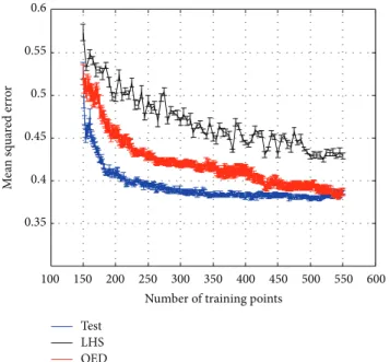
Figure 13 showed the hypersurface of 𝐶𝑝 as a function 𝜃 and 𝛽 which will be used to create the test data set for the design procedure. The G-optimal design procedure will be compared against the traditional LHS design procedure. An initial sample of 100 training points was chosen by LHS to start the design procedure. Surrogates were constructed by SFA using increasing number of LHS training points with increment of 5 points till a training set size of 500 was reached. For each training set size the training-testing procedure was repeated 10 times to eliminate any bias due to selection of training points and the mean and standard error of prediction accuracies were computed. The test set was constructed by the data-model fusion procedure. CFD solutions were constructed with a𝛽 increment of 1 degree and a𝜃 increment of approximately 6 degrees. The wind tunnel experiment used𝛽 increments of 4 degrees and four pressure sensors. The resulting test set had 20577 (= 361× 57) points which captured the𝐶𝑝variation in detail.
To implement the G-optimal design procedure, the stop-ping criteria discussed in Section 4 were used. This ensured that the FIM would not be singular. Also as the number of training points is increased the number of basis functions will also increase and address the bias problem. The lower bound on the RBF width parameter was constrained to1𝑒 − 64 and the center selection heuristic corresponding to the maximum absolute value of the residual was chosen. The basis centers were not optimized to save computational expense. One point was added to the training set at each iteration till 500 training points were collected. Again, to put the performance of the active learning procedure in perspective, its performance was also compared to the scenario when it is assumed that the true model is known and one point is chosen at each iteration. This corresponds to the maximum squared error of the current surrogate model.
It was also realized that additional information could also be incorporated in the training set for this problem.𝐶2𝑝bears peaks that correspond to those combinations of𝜃 and 𝛽 that result in maximum flow separation. Due to the geometry of the RALS tower bluff body, sensors on each wall measure the lowest pressures when the freestream wind is directed against the adjacent wall.
This physical phenomenon was used to enhance the information contained in the training set by adding points where𝛽 = [−180, −90, 0, 90, 180] degrees. Result for this case, shown in Figure 14, displays that active learning improves upon the LHS data collection method. Figure 15 shows the𝐶2𝑝 training points chosen by the G-optimal design procedure. The regions of the input domain corresponding to significant
100 150 200 250 300 350 400 450 500 550 600 0.35 0.4 0.45 0.5 0.55 0.6
Number of training points Test LHS OED M ea n s q ua re d er ro r
Figure 14: Reduction of mean squared error with increasing number of training points. Bars show standard error.
Pressure position angle (rad) −4 −4 −3 −3 −2 −2 −1 −1 0 0 1 1 2 2 3 3 4 4 Y aw a n gle (rad)
Figure 15: Training points chosen by the G-optimal design proce-dure.
functional variation are efficiently covered by the design algorithm corroborating the claims of Optimal Experiment Design.
5. Conclusions
This work was devoted to studying the compatibility of flush air data systems with bluff bodies with arbitrary geometries. Nontrivial geometries and requirements for efficient real time usage resulted in a challenging inverse problem of determin-ing air data parameters from surface pressure measurements that could be best solved by intelligent data driven algo-rithms. A data driven algorithm was developed based on the principles of scattered data approximation. It was proposed
that mathematical models can be utilized as a surrogate that solves the forward problem of generating pressure values from known wind speed and direction configuration. This surrogate can be used in conjunction with an array of flush mounted pressure taps to act as an air data measurement system. The proposed scattered data approximation algo-rithm, called Sequential Function Approximation (SFA), is a greedy self-adaptive function approximation tool that results in reliable and robust estimates without any user dependent control or kernel hyperparameter selection. In particular, a nonparametric and adaptive scattered data approximation tool accurately and efficiently mapped wind speed and yaw angle to pressure measurements taken from all four sides of the body. SFA was also used to reduce uncertainty in the wind tunnel tests by fusing data with low fidelity and smooth CFD models. Finally, to accelerate through the test matrices an intelligent sampling strategy was developed using principles of sequential experiment design.
Appendix
Sequential Function Approximation
Approximation of the unknown target function 𝑦 is con-structed by noting that a continuous𝑑-dimensional function can be arbitrarily well approximated by a linear combination of radial basis functions 𝜙. Sequential Function Approxi-mation (SFA) was developed from mesh-free finite element research but shares similarities with the Boosting [34] and Matching Pursuit [35] algorithms. SFA was developed earlier for regression and classification problems [16] and it is presented here for completeness. Approximation of the target vector𝑦 is constructed by utilizing the Gaussian radial basis function𝜙:
𝑦𝑎𝑛 =∑𝑛 𝑖=1
𝑐𝑖(𝜙 (𝑥, 𝛽𝑖) + 𝑏𝑖)
with𝜙 (𝑥, 𝛽𝑖) = exp [log [𝜆𝑖] (𝑥 − 𝑥∗𝑖) ⋅ (𝑥 − 𝑥∗𝑖)] for0 < 𝜆𝑖< 1.
(A.1)
Traditionally, Gaussian radial basis functions are written as
𝜙 (𝑥, 𝛽𝑖) = exp [−(𝑥 − 𝑥∗𝑖) ⋅ (𝑥 − 𝑥∗𝑖) 𝜎2
𝑖
] . (A.2)
Radial basis function is written as (A.1) in order to set up the optimization problem for𝜆𝑖as a bounded nonlinear line search instead of an unconstrained minimization problem for 𝜎𝑖. The basic principles of our greedy algorithm are moti-vated by the similarities between the iterative optimization procedures of Jones [36, 37] and Barron [38] and the Method of Weighted Residuals (MWR), specifically the Galerkin
method [39]. The function residual vector 𝑛⃗𝑟 at the𝑛th stage of approximation can be written as in
⃗𝑟
𝑛= 𝑦 (𝑥) − 𝑦𝑛𝑎(𝑥)
= 𝑦 (𝑥) − 𝑦𝑛−1𝑎 (𝑥) − 𝑐𝑛(𝜙 (𝑥, 𝛽𝑛) + 𝑏𝑛)
= ⃗𝑟𝑛−1− 𝑐𝑛(𝜙 (𝑥, 𝛽𝑛) + 𝑏𝑛) = ⃗𝑟𝑛−1− 𝑐𝑛( ⃗𝜙𝑛+ 𝑏𝑛) . (A.3)
Using the Petrov-Galerkin approach, a coefficient 𝑐𝑛 is selected that will force the function residual to be orthogonal to the basis function and𝑏𝑛using the discrete inner product ⟨, ⟩𝐷given by ⃗𝑟 𝑛⋅ ( ⃗𝜙𝑛+ 𝑏𝑛) = 𝑠 ∑ 𝑗=1 𝑟𝑛(𝑥𝑗) (𝜙𝑛(𝑥𝑖, 𝛽𝑛) + 𝑏𝑛) = ⟨ ⃗𝑟𝑛, ( ⃗𝜙𝑛+ 𝑏𝑛)⟩𝐷= − ⟨ ⃗𝑟𝑛,𝜕 ⃗𝑟𝜕𝑐𝑛 𝑛⟩𝐷 = −1 2 𝜕 ⟨ ⃗𝑟𝑛, ⃗𝑟𝑛⟩𝐷 𝜕𝑐𝑛 = 0 (A.4)
which is equivalent to selecting a value of 𝑐𝑛 that will minimize⟨ ⃗𝑟𝑛, ⃗𝑟𝑛⟩𝐷. Writing (A.3) as (A.5) where𝑔𝑛 = 𝑐𝑛⋅ 𝑏𝑛:
⃗𝑟
𝑛= ⃗𝑟𝑛−1− 𝑐𝑛 𝑛⃗𝜙 − 𝑔𝑛. (A.5) Expanding⟨ ⃗𝑟𝑛, ⃗𝑟𝑛⟩𝐷and taking the derivative with𝑐𝑛, we get
⟨ ⃗𝑟𝑛, ⃗𝑟𝑛⟩𝐷= ⟨ ⃗𝑟𝑛−1, ⃗𝑟𝑛−1⟩𝐷+ 𝑐𝑛2⟨ ⃗𝜙𝑛, ⃗𝜙𝑛⟩𝐷+ 𝑠𝑔2𝑛 − 2𝑐𝑛⟨ ⃗𝑟𝑛−1, ⃗𝜙𝑛⟩𝐷− 2𝑔𝑛⟨ ⃗𝑟𝑛−1⟩𝐷 + 2𝑐𝑛𝑔𝑛⟨ ⃗𝜙𝑛⟩𝐷, 𝜕 ⟨ ⃗𝑟𝑛, ⃗𝑟𝑛⟩𝐷 𝜕𝑐𝑛 = 2𝑐𝑛⟨ ⃗𝜙𝑛, ⃗𝜙𝑛⟩𝐷− 2 ⟨ ⃗𝑟𝑛−1, ⃗𝜙𝑛⟩𝐷 + 2𝑔𝑛⟨ ⃗𝜙𝑛⟩𝐷= 0, 𝑐𝑛= ⟨ ⃗𝑟𝑛−1, ⃗𝜙𝑛⟩𝐷− 𝑔𝑛⟨ ⃗𝜙𝑛⟩𝐷 ⟨ ⃗𝜙𝑛, ⃗𝜙𝑛⟩𝐷 . (A.6) Taking the derivative of⟨ ⃗𝑟𝑛, ⃗𝑟𝑛⟩𝐷with𝑔𝑛relates𝑐𝑛and𝑔𝑛in
𝜕 ⟨ ⃗𝑟𝑛, ⃗𝑟𝑛⟩𝐷
𝜕𝑔𝑛 = 2𝑠𝑔𝑛− 2 ⟨ ⃗𝑟𝑛−1⟩𝐷+ 2𝑐𝑛⟨ ⃗𝜙𝑛⟩𝐷= 0, 𝑔𝑛 =⟨ ⃗𝑟𝑛−1⟩𝐷− 𝑐𝑛⟨ ⃗𝜙𝑛⟩𝐷
𝑠 .
(A.7)
Substitute𝑔𝑛in (A.6) and solve for𝑐𝑛in
𝑐𝑛= (𝑠 ⟨ ⃗𝜙𝑛, ⃗𝑟𝑛−1⟩𝐷− ⟨ ⃗𝑟𝑛−1⟩𝐷⟨ ⃗𝜙𝑛⟩𝐷)
(𝑠 ⟨ ⃗𝜙𝑛, ⃗𝜙𝑛⟩𝐷− ⟨ ⃗𝜙𝑛⟩𝐷⟨ ⃗𝜙𝑛⟩𝐷) . (A.8) Since𝑏𝑛= 𝑔𝑛/𝑐𝑛, (A.9) gives𝑏𝑛:
𝑏𝑛= (⟨ ⃗𝑟𝑛−1⟩𝐷⟨ ⃗𝜙𝑛, ⃗𝜙𝑛⟩𝐷− ⟨ ⃗𝜙𝑛⟩𝐷⟨ ⃗𝜙𝑛, ⃗𝑟𝑛−1⟩𝐷) (𝑠 ⟨ ⃗𝜙𝑛, ⃗𝑟𝑛−1⟩𝐷− ⟨ ⃗𝑟𝑛−1⟩𝐷⟨ ⃗𝜙𝑛⟩𝐷)
. (A.9) The discrete inner product⟨ ⃗𝑟𝑛, ⃗𝑟𝑛⟩𝐷, which is equivalent to the square of the discrete𝐿2norm, can be rewritten, with the substitution of (A.8) and (A.9), as
𝑠 ∑ 𝑗=1 𝑟𝑛(𝑥𝑗) 𝑟𝑛(𝑥𝑗) = ⃗𝑟𝑛22,𝐷= ⟨ ⃗𝑟𝑛, ⃗𝑟𝑛⟩𝐷, ⟨ ⃗𝑟𝑛, ⃗𝑟𝑛⟩𝐷= ⟨ ⃗𝑟𝑛−1−⟨ ⃗𝑟𝑛−1⟩𝐷 𝑠 , 𝑟𝑛−1− ⟨ ⃗𝑟𝑛−1⟩𝐷 𝑠 ⟩𝐷 ⋅ (1 − ⟨ ⃗𝑟𝑛−1− ⟨ ⃗𝑟𝑛−1⟩𝐷/𝑠, ⃗𝜙𝑛− ⟨ ⃗𝜙𝑛⟩𝐷/𝑠⟩ 2 𝐷 ⟨ ⃗𝜙𝑛− ⟨ ⃗𝜙𝑛⟩𝐷/𝑠, ⃗𝜙𝑛− ⟨ ⃗𝜙𝑛⟩𝐷/𝑠⟩𝐷⟨ ⃗𝑟𝑛−1− ⟨ ⃗𝑟𝑛−1⟩𝐷/𝑠, ⃗𝑟𝑛−1− ⟨ ⃗𝑟𝑛−1⟩𝐷/𝑠⟩𝐷) . (A.10)
Recalling the definition of the cosine given by (A.11), using arbitrary functions 𝑓 and V and the discrete inner product,
cos(𝜃) = ⟨𝑓, V⟩𝐷 ⟨𝑓, 𝑓⟩𝐷1/2⟨V, V⟩𝐷1/2
. (A.11)
Equation (A.10) can be written as
⃗𝑟𝑛𝐷2,𝐷 = ⟨ ⃗𝑟𝑛−1−⟨ ⃗𝑟𝑛−1⟩𝐷 𝑠 , ⃗𝑟𝑛−1− ⟨ ⃗𝑟𝑛−1⟩𝐷 𝑠 ⟩ sin2(𝜃𝑛) = ( ⃗𝑟𝑛−1𝐷2,𝐷− ⟨ ⃗𝑟𝑛−1⟩2𝐷 𝑠 [2 − 1 𝑠]) sin2(𝜃𝑛) , (A.12)
where𝜃𝑛is the angle between ⃗𝜙𝑛and 𝑛−1⃗𝑟 since⟨ ⃗𝑟𝑛−1⟩𝐷/𝑠 and ⟨ ⃗𝜙𝑛⟩𝐷/𝑠 are scalars. With (A.12) one can see that ‖ ⃗𝑟𝑛‖2
2,𝐷 < ‖ ⃗𝑟𝑛−1‖2
2,𝐷as long as𝜃𝑛 ̸= 𝜋/2, which is a very robust condition for convergence. By inspection, the minimum of (A.12) is𝜃𝑛= 0, implying
𝑐𝑛(𝜙 (𝑥𝑖, 𝛽𝑛) + 𝑏𝑛) = 𝑟𝑛−1(𝑥𝑖) for 𝑖 = 1, . . . , 𝑠. (A.13) Therefore, to force| ⃗𝑟𝑛|22,𝐷 → 0 with as few stages 𝑛 as possi-ble, a low dimensional function approximation problem must be solved at each stage. This involves a bounded nonlinear minimization of (A.10) to determine the two variables𝜆𝑖 (0 < 𝜆𝑖 < 1) and index 𝑗∗ (𝑥∗
𝑛 = 𝑥𝑗 ∈ R𝑑) for the basis function center taken from the training set. The dimensionality of the nonlinear optimization problem is kept low since only one basis function needs to be solved at a time. To implement the SFA algorithm the user takes the following steps:
(1) Initiate the algorithm with the labels of the training data 0⃗𝑟 = {𝑦(𝑥1), . . . , 𝑦(𝑥𝑠)}.
(2) Basis center selection: Search the components of 𝑛−1⃗𝑟 for the maximum magnitude. Record the component index𝑗∗.
(3)𝑥∗𝑛 = 𝑥𝑗∗.
(4) Basis width optimization: With 𝑛⃗𝜙 centered at 𝑥∗𝑛, minimize (A.10) using optimization methods for bounded line search problems.
(5) Coefficient calculation: Calculate the coefficient𝑐𝑛and 𝑏𝑛from (A.8) and (A.9), respectively.
(6) Residual update: Update the residual vector 𝑛⃗𝑟 = ⃗𝑟𝑛−1− 𝑐𝑛( ⃗𝜙𝑛+𝑏𝑛). Repeat steps (3) to (6) until the termination criterion max| ⃗𝑟𝑛| ≤ 𝜏 has been met.
Our SFA method is linear in storage with respect to 𝑠 since it needs to store only𝑠 + 𝑠𝑑 vectors to compute the residuals: one vector of length𝑠(𝑟𝑛) and 𝑠 vectors of length 𝑑 (𝜉1, . . . , 𝜉𝑠) where 𝑠 is the number of samples and 𝑑 is the number of dimensions. To complete the SFA surrogate requires two vectors of length𝑛 ({𝑐1, . . . , 𝑐𝑛} and {𝑏1, . . . , 𝑏𝑛}) and𝑛 vectors of length 𝑛 + 1 (𝜂1, . . . , 𝜂𝑛). The dimensionality of the nonlinear optimization problem is kept low since we are solving only one basis at a time. Also, Meade and Zeldin [40] showed that, for bell-shaped basis functions, the minimum convergence rate is
𝑟𝑛22≅ ⟨𝑟𝑛, 𝑟𝑛⟩𝐷= exp [𝜅1− 𝜅2𝑛] where 𝑛 ≥ 2, (A.14) for positive constants 𝜅1 and 𝜅2. Equation (A.14) shows that, for minimum convergence, the logarithm of the inner product of the residual is a linear function of the number of bases (𝑛), which establishes an exponential convergence rate that is independent from the number of input dimensions (𝑑). For a detailed discussion and comparison of SFA with other state-of-the-art learning tools for regression and classification problems, please refer [41, 42].
Nomenclature
𝑏𝑛,𝑏1𝑛,𝑏2𝑛: 𝑛th bias in the approximation
𝑐𝑛,𝑐1𝑛,𝑐2𝑛: 𝑛th linear coefficient in the approximation 𝐶𝑝: Coefficient of pressure =𝑃/𝑞
𝑑: Input dimension 𝑓: Arbitrary function fps: Feet per second
𝐹: Forward mapping function 𝐺: Inverse mapping function 𝑛: Number of bases
𝑃, 𝑞: Static gauge pressure and dynamic pressure
𝑟𝑛: 𝑛th stage of the function residual R: Real coordinate space
R𝑑: 𝑑-dimensional vector space 𝑠: Number of training samples 𝑢(𝜉): Target function
𝑢𝑎𝑛(𝜉): 𝑛th stage of the target function approximation
𝑉∞: Freestream wind speed
⟨𝑓, V⟩𝐷: ∑𝑠𝑖(𝑓𝑖V𝑖) = discrete inner product of 𝑓 and V |𝑓|: Absolute value of𝑓 ‖𝑓‖2: (∫Ω𝑓2𝑑𝜉)1/2=𝐿2norm of𝑓 ‖𝑓‖2,𝐷: (∑𝑠𝑖(𝑓𝑖)2)1/2= discrete𝐿2norm of𝑓. Greek Symbols 𝛽: Yaw angle
𝜂: Set of nonlinear optimization parameters 𝜀: Objective function
𝜃: Polar coordinate
𝜆: Width parameter of Gaussian basis function 𝜉: 𝑑-dimensional input of the target function 𝜉𝑖: 𝑖th sample input of the target function 𝜉∗
𝑛: Sample input with component index𝑗∗at the nth stage 𝜏: User specified tolerance
𝜙: Basis function ]: Arbitrary function 𝛿: Input sensitivity 𝜌: Density. Subscripts 𝑖: Dummy index 𝑗∗: Component index of𝑟 (𝑛−1)with the maximum magnitude
𝑛: Associated with the number of bases 𝑠: Associated with the number of samples ∞: Associated with freestream conditions.
Superscripts
𝑎: Associated with the approximation 𝑑: Associated with the input dimension.
Conflict of Interests
The authors declare that there is no conflict of interests regarding the publication of this paper.
![Figure 1: Flush air data system installation at the nose of the F-18 Systems Research Aircraft [1].](https://thumb-eu.123doks.com/thumbv2/123doknet/14427263.514472/3.900.180.725.103.726/figure-flush-data-installation-nose-systems-research-aircraft.webp)
![Figure 4: (a) Wind tunnel model of the RALS tower [7] and (b) actual image of the RALS tower.](https://thumb-eu.123doks.com/thumbv2/123doknet/14427263.514472/5.900.238.661.109.430/figure-wind-tunnel-model-rals-tower-actual-image.webp)