HAL Id: inserm-00320828
https://www.hal.inserm.fr/inserm-00320828
Submitted on 18 May 2009
HAL is a multi-disciplinary open access
archive for the deposit and dissemination of
sci-entific research documents, whether they are
pub-lished or not. The documents may come from
teaching and research institutions in France or
abroad, or from public or private research centers.
L’archive ouverte pluridisciplinaire HAL, est
destinée au dépôt et à la diffusion de documents
scientifiques de niveau recherche, publiés ou non,
émanant des établissements d’enseignement et de
recherche français ou étrangers, des laboratoires
publics ou privés.
Transitions between secondary structures in isolated
polyalanines
Florent Calvo, Pierre Poulain
To cite this version:
Florent Calvo, Pierre Poulain. Transitions between secondary structures in isolated polyalanines. The
European Physical Journal D : Atomic, molecular, optical and plasma physics, EDP Sciences, 2009,
51 (1), pp.15-23. �10.1140/epjd/e2008-00096-0�. �inserm-00320828�
(will be inserted by the editor)
Transitions between secondary structures in isolated polyalanines
F. Calvo1
and P. Poulain2
1
Universit´e Claude Bernard Lyon 1 and CNRS, LASIM, Bˆat. A. Kastler, 43 Bd du 11 Novembre 1918, F69622 Villeurbanne cedex
2
EBGM, INSERM UMR-S 726, Universit´e Paris Diderot - Paris 7, 2 Place Jussieu, Case 7113, 75251 Paris cedex 05, France Received: / /2007 / Revised version: / /
Abstract. Monte Carlo simulations of gas-phase polyalanine peptides have been carried out with the Amber ff96force field. A low-temperature structural transition takes place between the α-helix stable conformation and β-sheet structures, followed by the unfolding phase change. The transition state ensembles connect-ing the helix and sheet conformations are investigated by samplconnect-ing the energy landscape along specific geometric order parameters as putative reaction coordinates, namely the electric dipole µ, the end-to-end distance d, and the gyration radius Rg. By performing series of shooting trajectories, the committor prob-abilities and their distributions are obtained, revealing that only the electric dipole provides a satisfactory transition coordinate for the α ↔ β interconversion. The nucleus at the transition is found to have a high helical content.
PACS. 64.60.Cn Order-disorder transformations; statistical mechanics of model systems – 02.70.Uu Ap-plications of Monte Carlo methods – 87.14.Ee Proteins
1 Introduction
The structure of proteins is closely related to their biologi-cal function. In many cases, the possibility to undergo con-formational transitions can be another important property for the function to be fully acquired, e.g. for transport [1] or motor [2,3] proteins, or in enzymes [4]. Misfolding of some proteins is due to an unwanted conformational change into a wrong, non-native structure often leading to fatal diseases. Prion proteins and the native Aβ peptide in Alzheimer’s disease are two important examples of α-helix-rich proteins which change to β-sheet upon aggrega-tion into the so-called amyloid fibrils [5]. The competiaggrega-tion between α helices and β sheets is also observed in proteins with nonhierarchical folding, as in β-lactoglobulin where α-helix intermediates are seen as transient conformations during folding into the β-sheet native structure [6].
While experimental methods such as high-resolution X-ray or NMR can often characterize the end states of a conformational change in solution, the entire pathway is much harder to study. Fluorescence resonance energy transfer provides detailed information about specific in-termolecular distances and their time evolution, however these partial data are far from full atomistic accuracy. In the gas phase, several methods have been developed during the last decade to get insight into the structural properties of proteins as an alternative to the solvent or matrix characterizations. Studying isolated biomolecules also has the advantage of putting aside the intermolecu-lar interactions, thus simplifying greatly the analysis [7]. Infrared spectroscopy [8–10], ion mobility [11,12], H/D
exchange reactions [13], peptide fragmentation [13–15] or electric dipole measurements [16] have all contributed sig-nificantly to our understanding of gas-phase peptides. In particular, the existence of the α-helix and β-sheet con-formations has been attested in a number of cases [17]. Yet, determining transition pathways remains an issue in vacuo, and the results of computer simulations can be in-valuable.
Conformational changes in silico can be addressed in a number of ways, depending on the precise aims. Direct molecular dynamics [18–23] and Monte Carlo (MC) sim-ulations [24–27] provide useful insight into the energet-ics and kinetenerget-ics of the folding transition, especially in the case of polyalanines. However, in their basic form they are usually not appropriate for studying rare events involving large free energy barriers. From the structural point of view, one would like to characterize not only the two end states, but also the optimal set of reaction coordinates along which the transition is best visualized. The com-mon approach here is intuition, by selecting a priori order parameters defined according to the molecular geometry, and by calculating the probability distribution of finding these variables and the corresponding free energy maps. Upon identification of barriers between the two states, ad-ditional trajectories can be run to calculate the rate con-stants via transition path sampling (TPS) [28,29] or re-lated schemes [30–32]. More recently, several groups [33– 36] have proposed improvements of the pioneering TPS method in which the quality of the reaction coordinate is assessed by computing the committor probability pc, that
2 F. Calvo and P. Poulain: Transitions between secondary structures
than in the other state. This quantity, though it may not appear immediately physical, allows a proper definition of a transition state as the set of conformations for which pc= 1/2.
In a previous work, we have theoretically shown that gas-phase polyalanines can exhibit a thermally stable β-sheet intermediate between the low-temperature α-helical native state and the high-temperature unfolded state [37]. These results are consistent with experimental measure-ments [38] and also with previous theoretical suggestions from other groups [39–41]. Here we focus on the α-helix ↔ β-sheet interconversion, which we attempt to characterize in terms of specific order parameters. More precisely, we have chosen the electric dipole µ, the end-to-end distance d between the N-terminal atom and the H atom from the hydroxyl group in the carbonyl terminal, and finally the gyration radius Rg. Near the α–β equilibrium transition
temperature, the free energies along these three parame-ters show stable basins corresponding to both conforma-tions. However, as will be seen below, dividing surfaces are not straightforward to identify and, more importantly, they may not reflect the true transition states. By shooting many trajectories from several regions of the energy land-scape, the committor probabilities can be calculated, thus helping in assessing the relevances of these order parame-ters as reaction coordinates for the α ↔ β interconversion. The article is organized as follows. In the next section, we describe all the computational methods used to sample the potential energy surface of our model system, the iso-lated octa-alanine. The equilibrium results and the tran-sition state ensembles associated with each of the three order parameters are critically discussed in Sec. 3, and some concluding remarks are finally given in Sec. 4.
2 Methods
We have chosen a short enough polyalanine that is found stable in both the α-helical and β-hairpin configurations, namely the octa-alanine system. This peptide is modelled using the Amber ff96 force field [42]. Because the original parameters of Amber ff96 were originally fitted to repro-duce the properties of hydrated biomolecules, the partial charges had to be increased to account for polarization effects. When used in the gas phase, this parameter set overstabilizes β-sheet structures with respect to helices [44]. To circumvent this problem and shield the charges, a dielectric constant εr= 2 was used in the simulations, thus
satisfactorily reproducing the electric dipole measured in deflection experiments [43].
We have used two kinds of methods in this work. A first goal is to sample the energy landscape of our polypeptide at thermal equilibrium, in order to characterize the α ↔ β interconversion and to calculate Landau free-energy curves corresponding to specific order parameters. In a second part, the quality of these order parameters as suitable reaction coordinates will be assessed by shooting trajec-tories from putative transition states and estimating the committor averages and their probability distributions.
2.1 Sampling the energy landscape
The potential energy surface of the octa-alanine was ex-plored using parallel tempering (PT) Monte Carlo simula-tions as a reference. 32 replicas were propagated simulta-neously in the temperature range 50 K ≤ T ≤ 1000 K with a geometric progression. Ten series of 106
Monte Carlo cycles per replica were propagated consecutively, the last configurations of each simulation providing the starting conditions for the next one. Here one MC move consisted of randomly selecting one torsion angle of the backbone or side chains, and randomly rotating it by an angle δθ drawn from a range [−θmax, θmax], with θmax
ad-justed at each temperature to get approximately 50% ac-ceptance rate according to the Metropolis rule. Here one MC cycle is a series of 23 consecutive MC moves. After each cycle, one exchange between two random adjacent replicas was attempted with 10% probability.
While the average potential energy hEi or its fluctua-tions h∆E2
i suffice to monitor the unfolding transition, other quantities are required to locate the presence of α-helix or β-sheet secondary structures. We thus calcu-lated the electric dipole vector µ and its modulus µ, the end-to-end distance d between the nitrogen atom in N-ter position and the hydrogen atom from the hydroxyl group in C-ter position, as well as the gyration radius Rg. In addition to the standard thermal averages hµi,
hdi and hRgi, we recorded the two-dimensional histograms
hT(E, A) as a function of potential energy and geometric
parameter A = µ, d or Rg at the temperature T . These
histograms were then processed into the joint densities of states Ω(E, A), and subsequently into the thermal aver-ages hEi, hAi or their fluctuations as a continuous function of temperature, via a multiple histogram analysis.
Complementary Monte Carlo simulations were perfor-med using the Wang-Landau (WL) procedure [45] for joint densities of states, recently improved using our annealing scheme [46]. Here the two-dimensional density of states Ω(E, A) is numerically calculated with increasing accu-racy by penalizing each visited state more and more as it is being visited during the exploration. This algorithm eventually converges to the true density of states, which in turns provides all thermodynamical properties in the canonical ensemble after Laplace transformation.
The two-dimensional Wang-Landau method, previous-ly used with the electric dipole as the extra variable A, was found to perform very well for small peptides [46] when compared with parallel tempering Monte Carlo. Here we have chosen to repeat these simulations in the same con-ditions, but with the end-to-end distance d and the gyra-tion radius Rg as the two extra variables to the potential
energy E. The simulation details for these Wang-Landau simulations are the same as in Ref. [46], and will not be further detailed here. In particular, the inverval in A was discretized into 200 bins for the three variables and the en-ergy interval consisted of 300 bins. The ranges for the three geometric variables were 0 ≤ µ ≤ 40 D, 0 ≤ d ≤ 35 ˚A, and 4 ˚A≤ Rg≤ 10 ˚A, respectively.
The microcanonical densities of states Ω(E, A) can also be used to calculate the canonical probability of
find-ing the system with parameter A within some error dA at temperature T , again via a simple Laplace transformation:
p(A, T )dA ∝ dA Z
Ω(E, A) exp(−E/kBT )dE, (1)
with kB the Boltzmann constant. From the probability
p(A, T ), the Landau free energy F (A, T ) is defined at tem-perature T as
F (A, T ) = −kBT ln p(A, T ). (2)
Bistable systems are expected to show two minima in the Landau free energy as a function of a suitable function A. At the transition temperature, and for a first-order like phase transition, the two minima should have the same depth.
2.2 Transition state ensembles
The shape of the probability p(A, T ) or the free energy F (A, T ) provides a great deal of information about the sta-ble regions of the energy landscape, after projection onto the physically meaningful order parameters A. However, even the presence of two comparable minima in F (A, T∗)
near the equilibrium temperature T∗ does not qualify the
parameter A as a good reaction coordinate.
In order to determine whether the parameter A is an adequate transition coordinate, one must calculate the committor probability pc(A) at the barrier A†, that is the
probability that a trajectory initiated at A† will fall into
one minimum earlier than in the other minimum. By defi-nition, the transition region between the two minima is the isocommittor surface, or the set of points in phase space for which pc= 1/2. Therefore a necessary condition for A
to be a good transition coordinate is that the average com-mittor probability hpci taken for points having A ≃ A† is
close to one half. However, as discussed in particular by Best and Hummer [35] and by Geissler and coworkers [47], this necessary condition on the average hpci over a set of
configurations is not sufficient. It may recover situations where this set actually comprises of state points already belonging to the two end states, resulting in an appar-ent free energy barrier only after projecting onto a wrong coordinate and further statistical averaging. A more rigor-ous approach is to calculate the distribution P(pc) of the
probability pc after repeating the calculation of pc from
many different starting points at A†. If P(p
c) has a peaked
shape centered at 1/2, then the variable A can be consid-ered as a suitable reaction coordinate for the transition [35,47]. Conversely, a bimodal distribution P(pc) peaked
at the extremities pc = 0 and pc = 1 cannot be
consid-ered as appropriate. This situation was illustrated by Du and coworkers [48] who found that neither the number of native contacts nor the looplength distributions could de-scribe the folding transition of lattice models of proteins. For the present system, we have first sampled sets of transition points by saving configurations corresponding to the desired value of A0within some small range ±δA/2,
selecting A0near the maximum of the free energy barrier
A† separating the α-helix and β-sheet minima. This
sam-pling was carried out using the parallel tempering Monte Carlo simulations without any bias for the parameters d and Rg. Sampling configurations according to their
elec-tric dipole turned out to be more difficult, due to the much higher energy barriers reflecting very low occurence prob-abilities. For this parameter, and following the suggestion of Best and Hummer [35], an harmonic umbrella poten-tial W (µ) = k(µ − µ0)
2
around the desired value µ0 was
added to the potential energy, with the spring constant k = 5 kcal/mol/D2
.
Once a set {R}(A0) of N configurations
character-ized by their value of A(R) ∈ [A0 − δA/2, A0+ δA/2]
had been selected, the committor probabilities pc(R) were
estimated by shooting independent Monte Carlo trajec-tories initiated from each of these configurations. These ’aimless’ shooting trajectories started at the temperature T = 150 K, which is below the folding temperature but above the α ↔ β interconversion, and after 5 × 10⁴
MC cycles the temperature was decreased to 80 K for another quenching round of 5 × 10⁴
MC cycles. For each starting configuration R, the number M of trajectories converging to either of the α-helical or β-sheet states after the 105
MC cycles was required to be 50. If one simulation did not end into one of these states before the 105
MC cycles, then it was just ignored and a new independent simulation was restarted. The committor probability pc is here given by
the number Mβ/M of trajectories ending in the β-sheet
state, divided by the total number M = Mα+ Mβof
tra-jectories. The different values pc obtained for N = 250
representative configurations of the order parameters A close to A0 subsequently provide the distribution P(pc)
used to assess the quality of A as a good transition coor-dinate.
3 Results and discussion
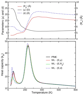
3.1 Equilibrium propertiesThe variations of the heat capacities of the octa-alanine obtained using the parallel tempering and Wang-Landau Monte Carlo simulations are represented in Fig. 1. The thermally averaged electric dipole hµi, end-to-end distance hdi and radius of gyration hRgi found for the reference
parallel tempering Monte Carlo simulations are also shown in this figure. All heat capacity curves exhibit two peaks, the large peak centered near 215 K being robust for all other WL simulations. At this temperature, the gyration radius and the end-to-end distance sharply increase, as a signature of the unfolding transition.
The low-temperature peak centered near T∗= 80 K is
characterized by a drop in both hµi and hdi, but a small increase in hRgi. The most stable conformation of the
pep-tide is an α-helix, which is associated with a high elec-tric dipole µ ≃ 24.5 D resulting from the alignment of intramolecular hydrogen bonds. The helical state has a significant end-to-end distance d ≃ 10 ˚A, but a reduced Rg ≃ 4.6 ˚A reflecting its compactness. β-hairpin
4 F. Calvo and P. Poulain: Transitions between secondary structures 0 5 10 15 20 25 30 Parameters 〈µ〉 and 〈 d 〉 〈µ〉 (D) 〈d〉 (Å) 4 5 6 7 8 9 10 〈 Rg 〉 (Å) 〈Rg〉 (Å) 0 200 400 600 800 Temperature (K) 10 20 30 40 50 Heat capacity (k B ) PTMC WL - (E,µ) WL - (E,Rg) WL - (E,d)
Fig. 1. Upper panel: thermally averaged dipole moment hµi, gyration radius hRgi, and end-to-end distance hdi of the Ala8 peptide as a function of temperature, obtained from parallel tempering MC simulations. Lower panel: canonical heat ca-pacity of the same system obtained from MC simulations, or from Wang-Landau simulations using joint densities of states on energy E and µ, Rg, or d as an extra order parameter.
end-to-end distance, but a slightly higher radius of gyra-tion. The stable state of the peptide thus changes from α-helical to β-sheet at the temperature where the heat capacity reaches its first peak. This stable β-sheet state can be further evidenced by calculating other structural indicators, such as the helical fraction or the fluctuations in the overlap function with the native state [49]. The presence of an intermediate β-sheet phase between the α-helical and unfolded random coil states is not specific to the octa-alanine, as longer alanine-rich peptides also exhibit this peculiar behaviour [37]. The β-sheet state is stabilized due to its higher entropy related to softer vibra-tional modes, whereas α-helices are energetically favored but more tightly bound [37,38]. If the peptide is hydrated, the helical conformation is stabilized by its favorable elec-trostatic interactions with the polarisable solvent. Most computer simulations of polyalanines in explicit or im-plicit solvent usually reported a single helix-coil transi-tion induced by temperature [18,21,22,24,25], matching the picture of the Zimm-Bragg model [50].
Having a closer examination at the low-temperature heat capacity peak, clear differences between the perfor-mances of the three Wang-Landau Monte Carlo simula-tions are found in comparison with the reference parallel tempering data. While using the (E, µ) order parameters
correctly reproduces the location, height and width of this peak, the same cannot be said about the two other flavors (E, d) and (E, Rg). Repeating the Wang-Landau
simula-tions from independent initial condisimula-tions, the results ob-tained with the latter two sets of variables are found to fluctuate significantly, whereas the density of states in E and µ is reproducible. These findings show that sampling with the d or Rg variables in addition to E is less efficient
than using the electric dipole. This, in turn, already sug-gests that neither d or Rg are reliable order parameters
to explore the conformation space corresponding to the α and β states and their transition. The relative efficacy of these order parameters will now be assessed by look-ing at free energy profiles and computlook-ing the committor probabilities.
3.2 Electric dipole as the transition coordinate
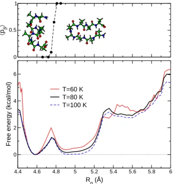
We first consider the Landau free energy as a function of the order parameter µ. The variations of F (µ) at the temperatures of 60, 80, and 100 K, near the α ↔ β equi-librium, are represented in Fig. 2. Here and in all other free energy calculations, the curves have been shifted such that their minimum is exactly at F = 0. At the three selected temperatures, the free energy curves exhibit two main minima near µ = 9 D and µ = 24.5 D, which cor-respond to the β-sheet and α-helical conformations, re-spectively. These minima have the same depth at T = T∗,
but at 60 K (100 K) the α state (β state) is more stable. The equal free energies of the two states at the transi-tion temperature confirm the first-order character of the α ↔ β interconversion. The barrier between the two states is located in the range µ ∼ 18–20 D, and is rather high (about 9 kcal/mol). Several sets of conformations have been sampled according to their electric dipole. Each set is characterized by its center µ and its width δµ = 0.2 D used as a tolerance factor during the selection. For a given set of conformations, Monte Carlo trajectories were shot until either of the α or β states was reached. In practice, the α-helical state is defined by its electric dipole µ, which must be larger than 22 D. Conformations are considered to be in the β-sheet state if µ ≤ 15 D and d ≤ 7 ˚A.
Varying µ in the range 17 D ≤ µ ≤ 23 D, the com-mittor probabilities pc are calculated by monitoring the
number of trajectories ending up in the β-sheet state ear-lier than in the α helical state. The averaged committor probability hpci is plotted in the upper panel of Fig. 2 as a
function of µ. This average value shows a steady decrease from 1 (for µ ≤ 17 D) to 0 (for µ ≥ 22 D). According to our definitions, any trajectory starting at a conformation with µ ≥ 22 D is already in the α state. For dipoles near µ ≃ 20.0 ± 0.1 D, the committor probability is about 0.5, indicating that conformations with this value of µ belong to the isocommittor surface, that is the optimal transition coordinate.
More insight into the quality of the electric dipole as reaction coordinate is provided by looking at the distribu-tions of committor probabilities, shown in Fig. 3 for three values of µ. These distributions are narrowly located near
0 0.5 1 〈 pβ 〉 0 5 10 15 20 25 30 µ (D) 0 2 4 6 8 10 12 14
Free energy (kcal/mol)
T=60 K T=80 K T=100 K
Fig. 2. Upper panel: average committor probability hpci(µ) of ending first in the sheet conformation, starting from a sam-ple of configurations with prescribed dipole moment µ. Lower panel: Landau free energy profiles along the µ order parameter, at temperatures close to the helix/sheet transition.
0 0.2 0.4 0.6 0.8 1 commitor probability 0 0.2 0.4 0.6 0.8 1 probability 17.9 ≤ µ ≤ 18.1 19.9 ≤ µ ≤ 20.1 20.9 ≤ µ ≤ 21.1
Fig. 3. Distribution of committor probabilities pcfor ending first in the sheet conformation, for trajectories initiated at con-formations with prescribed values of the dipole moment µ.
pc = 0 or 1 for µ = 21.0 ± 0.1 D and µ = 18.0 ± 0.1 D,
respectively. For µ = 20.0 ± 0.1 D, the distribution is sym-metrically peaked near pc= 0.5. This is the expected
be-havior for a good reaction coordinate at the transition state.
3.3 Radius of gyration as the reaction coordinate The Landau free energy profiles F (Rg) as a function of the
gyration radius are displayed in Fig. 4 for the same three
temperatures of 60, 80, and 100 K. Only the interval 4.4 ˚A ≤ Rg≤ 6 ˚A is shown as it relevant for both the α and β
states. The free energies have a minimum at each of these states. Contrary to the free energy curves as a function of the electric dipole, the two minima are not equally deep at the equilibrium temperature. However this is partly com-pensated by the much broader minimum of the β-sheet state (approximately 4.9 ˚A ≤ Rg ≤ 5.1 ˚A versus 4.58 ˚A
≤ Rg≤ 4.62 ˚A for the helical state). The free energy
bar-rier is close to Rg= 4.76 ˚A but is only moderate, around
1 kcal/mol. This significant difference in the energy barrier when changing the order parameter indicates that impor-tant orthogonal variables are missing in the description of the kinetics when selecting conformations based on their gyration radius only [29].
0 0.5 1 〈 pβ 〉 4.4 4.6 4.8 5 5.2 5.4 5.6 5.8 6 Rg (Å) 0 2 4 6
Free energy (kcal/mol)
T=60 K T=80 K T=100 K
Fig. 4. Upper panel: average committor probability hpci(Rg) of ending first in the sheet conformation, starting from a sam-ple of configurations with prescribed gyration radius Rg. Lower panel: Landau free energy profiles along the Rg order param-eter, at temperatures close to the helix/sheet transition.
Conformations have been sampled based on their value of Rg, for gyration radii in the range 4.66–4.85 ˚A and
δRg = 0.03 ˚A. The average committor probabilities,
rep-resented in the upper panel of Fig. 4 against Rg, sharply
increase as Rg crosses the barrier. The distributions of
committor probabilities corresponding to 4.75 ˚A ≤ Rg ≤
4.78 ˚A and 4.79 ˚A ≤ Rg ≤ 4.82 ˚A, for which hpci = 0.09
and 0.65, respectively, are shown in Fig. 5.
Both distributions are strongly bimodal with nonzero values only for pc= 0 and pc = 1. Hence the starting
con-formations of the shooting trajectories already lie in the α or β states, rathers than being actually located inbetween.
6 F. Calvo and P. Poulain: Transitions between secondary structures 0 0.2 0.4 0.6 0.8 1 commitor probability 0 0.2 0.4 0.6 0.8 1 probability 4.75 ≤ Rg≤ 4.78 4.79 ≤ Rg≤ 4.82
Fig. 5. Distribution of committor probabilities pcfor ending first in the sheet conformation, for trajectories initiated at con-formations with prescribed values of the gyration radius Rg.
The gyration radius appears as a very poor reaction coor-dinate for characterizing the α ↔ β transition.
3.4 End-to-end distance as the reaction coordinate The Landau free energy profiles F (d) obtained using the end-to-end distance d have been represented in Fig. 6, again at the same three temperatures. Conversely to the previous choices of order parameters, more than two min-ima are found in the variations of the free energy curves at the α/β equilibrium. The stable α-helical and β-sheet states are the deepest minima at the transition temper-ature of 80 K, they are located near d = 10.2 ˚A and d = 5.3 ˚A, respectively. The presence of extra metastable states at d = 8.1 ˚A and d = 11.5 ˚A makes it difficult to identify a clear barrier. Furthermore it would be de-sirable to characterize the conformations corresponding to the metastable minima, especially given that they are separated by rather small barriers (∼ 0.5 kcal/mol), hence being rather probable.
In this purpose, sets of conformations at selected val-ues of d within δd = 0.1 ˚A have been gathered near the three barriers in F (d), namely d = 6.9 ˚A, d = 9.0 ˚A, and d = 10.9 ˚A, as well as near the metastable minima themselves. The average committor probabilities hpci
cal-culated after repeating the shooting trajectories are repre-sented in Fig. 6 as a function of d. Quite strikingly, their variations are not monotonic with the order parameter: the chances of ending up in the β-hairpin conformations are high not only for d ≤ 9.0 ˚A, but also for d ≥ 10.9 ˚A. This is a straightforward consequence of how d is con-nected to the conformation. Low d distances usually be-long to the β-hairpin state. Torsions abe-long the backbone may break the alignment between the two strands, as seen on the typical conformation found at the barrier near d = 6.9 ˚A on Fig. 6. Very large values of d correspond to extended conformations, and are thus more likely to belong also to the basin of attraction of the β-sheet state.
0 0.5 1 〈 pβ 〉 2 4 6 8 10 12 14 d (Å) -1 0 1 2 3 4 5
Free energy (kcal/mol)
T=60 K T=80 K T=100 K
Fig. 6.Upper panel: average committor probability hpci(d) of ending first in the sheet conformation, starting from a sample of configurations with prescribed end-to-end distance d. Lower panel: Landau free energy profiles along the d order parameter, at temperatures close to the helix/sheet transition.
In the intermediate range 7.0 ˚A ≤ d ≤ 11.0 ˚A, confor-mations can be of the α-helical type with some degree of stretching, or of the β-sheet type with the two strands not perfectly parallel. Therefore the end-to-end distance is a good parameter only for characterizing β-hairpin con-formations, but it is not able to discriminate efficiently α helices from extended conformations, which more likely fold into β sheets due to their higher entropy.
0 0.2 0.4 0.6 0.8 1 commitor probability 0 0.2 0.4 0.6 0.8 probability 9.00 ≤ d ≤ 9.10 10.85 ≤ d ≤ 10.95
Fig. 7. Distribution of committor probabilities pc for ending first in the sheet conformation, for trajectories initiated at con-formations with prescribed values of the end-to-end distance d.
The distributions P(pc) of the committor probabilities
for which the averages are closest to 50%, that is d = 9.0 ˚A and 10.9 ˚A, are displayed in Fig. 7. As was the case for the gyration radius, the two distributions are essentially peaked at pc = 0 and pc = 1, indicating that the
confor-mations sampled according to their end-to-end distance often belong to either of the α or β states. It can be no-ticed, though, that the two peaks at pc= 0 and 1 are less
sharp for d = 9.0 ˚A. Therefore this set of conformations captures the true transition coordinate less approximately than the gyration radius.
3.5 Discussion
The Landau free energies obtained from Monte Carlo sim-ulations show important differences depending on the or-der parameter consior-dered. While the α-helix and β-sheet stable states appear on these curves as two well-defined minima, the barriers are not always easy to infer. Con-formations belonging to either of the α or β states do not differ significantly by their gyration radius, and the barrier between the free energy minima is particularly narrow. In the case of the end-to-end distance order parameter, ad-ditional minima corresponding to deformed sheet confor-mations and multiple barriers blur the picture of a simple two-state system. Only the electric dipole seems to resolve unambiguously helix and strand conformations.
The relative performances of the order parameters µ, Rg, and d to describe the α ↔ β interconversion, as
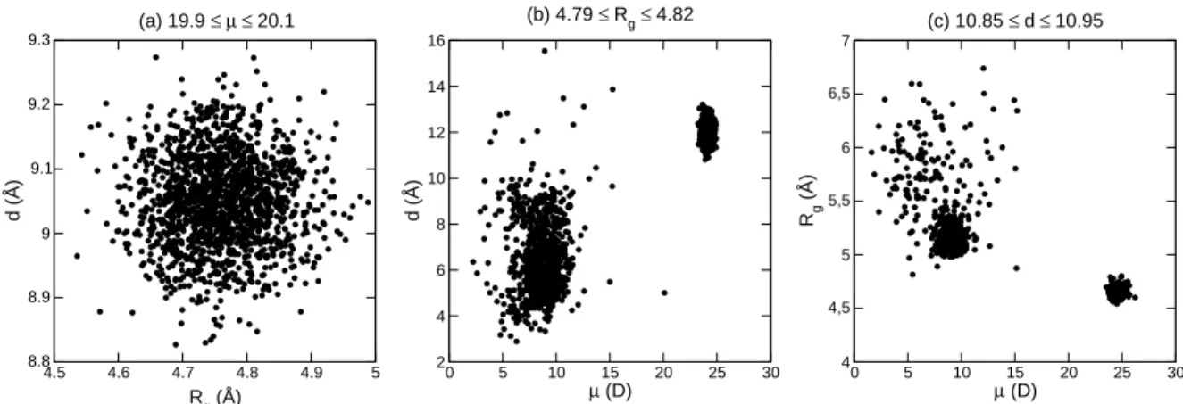
as-sessed by the distributions of committor probabilities at the isocommittor surface, clearly show that only the elec-tric dipole can play the role of a proper reaction coordinate for this transition. The strongly bimodal distributions of the committor probabilities found for the gyration radius and, albeit to a lesser extent, for the end-to-end distance, are related to the proximity of the selected conformations with respect to the α and β states. In contrast, the struc-tures sampled at the top of the free energy barrier in the electric dipole case are not as clearly associated to the end states. These observations can be further rationalized by considering the correlations between the two order pa-rameters remaining when selecting one of them among the three quantities (µ, Rg, d). In Fig. 8 these correlations are
represented for three order parameters near the isocom-mittor condition hpci = 1/2.
The correlation diagram obtained when selecting con-formations based on their electric dipole exhibits one sin-gle peak near Rg ≃ 4.7–4.8 ˚A and d = 8.9–9.2 ˚A.
Con-versely, conformations selected according to their radius of gyration or their end-to-end distance lead to two peaks which can be easily identified to either of the α or β states. Therefore, neither Rg nor d alone provide good reaction
coordinates for the α ↔ β transition. On the other hand, the electric dipole seems to be a satisfactory transition co-ordinate, and the Landau free energy F (µ) at T = 80 K can be used to determine the properties of the transition state.
The location of the barrier, near µ ≃ 20 D, is rather close to the helical state, rather than to the β-hairpin
basin. This is reflected on the strong assymetry in the free energy curves F (µ) shown in Fig. 2, in which the α-helix basin is much narrower than the broad β basin. Hence the conformations at the transition state have a high helical fraction. The formation of this helix core from a β-strand conformation, or the breaking of a small part of the full helix, are the rate limiting steps of the transition. On both sides of the barrier, the dipole varies over only about 2 D, with the substantial energy cost of 5–6 kcal/mol to reach the barrier top. This high energy barrier makes the α ↔ β interconversion unlikely to be observed in molecular dy-namics simulations, but could well take place in molecular beams with time-of-flights longer than a few microseconds.
4 Conclusion
As the elementary building blocks of proteins, helices and sheets are of primary importance in determining the fold-ing or misfoldfold-ing properties and associated functions of many biologically relevant systems. The archetypal poly-alanines studied here naturally fold into α helices, but can also form β-hairpin conformations by entropic stabiliza-tion. In the present work, the competition between the α and β secondary structures was studied from the perspec-tive of the transition pathways connecting them. Using dedicated Monte Carlo simulations, the α ↔ β intercon-version was first characterized by the Landau free ener-gies, which provide a picture of the energy landscape pro-jected onto specific order parameters. The electric dipole µ, the gyration radius Rg, and the end-to-end distance d
were used to monitor the transition near the equilibrium temperature for octa-alanine as found by our simulations based on the Amber ff96 force field. The variations of the free energy profiles usually show two clear minima as-sociated with each of the α and β states, from which a transition region is easily located at the barrier. However, the end-to-end distance is not such a good coordinate for structural characterization, because many conformations without any helical content share the same value of d as the helix state.
By sampling conformations at the putative transition barrier, trajectories were shot to estimate the committor probability pc to the β-hairpin basin. For all order
param-eters, suitable ranges were located leading to the isocom-mittor property pc = 1/2 which is required for the order
parameter to be a suitable reaction coordinate. However, the distributions of committor probabilities at the isocom-mittor surface reveal contrasting behaviors. Most confor-mations sampled at the barrier in Rgor d actually belong
to the α or β minima, whereas conformations at the bar-rier in µ are closer to real transition states. Therefore, only the latter order parameter provides a good reaction coordinate to describe the α ↔ β interconversion. The present results also showed that the transition state has a rather large extent of helicity, which further requires a high potential energy change of more than 5 kcal/mol.
The three order parameters used here were selected based on physical intuition. One possible extension of the present work could be to refine the reaction coordinate
8 F. Calvo and P. Poulain: Transitions between secondary structures 4.5 4.6 4.7 4.8 4.9 5 Rg (Å) 8.8 8.9 9 9.1 9.2 9.3 d (Å) (a) 19.9 ≤ µ ≤ 20.1 0 5 10 15 20 25 30 µ (D) 2 4 6 8 10 12 14 16 d (Å) (b) 4.79 ≤ Rg≤ 4.82 0 5 10 15 20 25 30 µ (D) 4 4,5 5 5,5 6 6,5 7 Rg (Å) (c) 10.85 ≤ d ≤ 10.95
Fig. 8.Correlation between the two remaining order parameters, for conformations taken at the transition state defined by the reaction coordinate in (a) dipole moment; (b) gyration radius; (c) end-to-end distance.
following the methods of previous groups [33–36], partic-ularly the automated schemes proposed by Ma and Din-ner [33] or Peters and Trout [36]. Optimizing the reaction coordinate would also improve the efficiency of sampling methods such as the Wang-Landau algorithm for joint densities of states, because the bottleneck of sampling pre-cisely lies in the crossing of the highest energy barriers. It would also be of interest to investigate larger polyalanines, to determine the extent of helicity in the transition states between α and β conformations. Beyond the competition between these secondary motifs, the folding transition it-self could be studied with the same set of methods and dedicated order parameters.
Acknowledgements
Computer simulations were carried out at the IDRIS and CINES computer centers, which we gratefully acknowl-edge. We also thank GDR 2758 for financial support. We thank Ph. Dugourd, R. Antoine, and M. Broyer for fruitful discussions.
References
1. M. Perutz, A. Wilkinson, M. Paoli, and G. Dodson, Annu. Rev. Biophys. Biomol. Struct. 27, 1 (1998).
2. M. Schliwa and G. Woehlke, Nature (London) 422, 759 (2003).
3. R. Mallik and S. Gross, Curr. Biol. 14, R971 (2004). 4. S. Benkovic and S. Hammes-Schiffer, Science 301, 1196
(2003).
5. J. W. Kelly, Curr. Opin. Struct. Biol. 8, 101 (1998). 6. D. Hamada, S. Segawa, and Y. Goto, Nat. Struct. Biol. 3,
868 (1996).
7. Special issue on Molecular Physics of Building Blocks of Life under Isolated or Defined Conditions, Eur. Phys. J. D 20, 309 (2002), edited by R. Weinkauf, J.-P. Schermann, M. S. de Vries, and K. Kleinermanns.
8. J. M. Bakker, L. M. Aleese, G. Meijer and G. von Helden, Phys. Rev. Lett. 91, 203003 (2003).
9. C. Kapota, J. Lemaire, P. Maˆıtre, and G. Ohanessian, J. Am. Chem. Soc. 126, 1836 (2004).
10. W. Chin, F. Piuzzi, I. Dimicoli, and M. Mons, Phys. Chem. Chem. Phys. 8, 1033 (2002).
11. M. F. Jarrold, Annu. Rev. Phys. Chem. 51, 179 (2000). 12. C. S. Hoaglund-Hyzer, A. E. Counterman, and D. E.
Clem-mer, Chem. Rev. 99, 3037 (1999).
13. H. Oh, K. Breuker, S. K. Sze, Y. Ge, B. K. Carpenter, and F. W. McLafferty, Proc. Natl. Acad. Sci. USA 99, 15863 (2002).
14. D. M. Horn, K. Breuker, A. J. Frank, and F. W. McLaf-ferty, J. Am. Chem. Soc. 123, 9792 (2001).
15. N. C. Polfer, K. F. Haselman, P. R. R. Langridge-Smith, and P. E. Barran, Mol. Phys. 103, 1481 (2005).
16. R. Antoine, I. Compagnon, D. Rayane, M. Broyer, Ph. Dugourd, G. Breaux, F. C. Hagemeister, D. Pippen, R. R. Hudgins, and M. F. Jarrold, J. Am. Chem. Soc. 124, 6737 (2002).
17. M. F. Jarrold, Phys. Chem. Chem. Phys. 9, 1659 (2007). 18. V. Daggett, P. A. Kollman, and I. D. Kuntz, Biopolymers
31, 1115 (1991).
19. S. Furoiscorbin, J. C. Smith, and R. Lavery, Biopolymers 35, 555 (1995).
20. W. Weber, P. H. Hunenberger, and J. A. McCammon, J. Phys. Chem. B 104, 3668 (2000).
21. Y. Z. Ohkubo and C. L. Brooks, Proc. Natl. Acad. Sci. USA 100, 13916 (2003).
22. S. Yang and M. Cho, J. Phys. Chem. B 111, 605 (2007). 23. W. Han and Y. D. Wu, J. Chem. Theory Comput. 3, 2146
(2007).
24. Y. Peng and U. H. E. Hansmann, Biophys. J. 82, 3269 (2002).
25. Y. Peng, U. H. E. Hansmann, and N. A. Alves, J. Chem. Phys. 118, 2374 (2003).
26. A. E. van Giessen and J. E. Straub, J. Chem. Phys. 122, 024904 (2005).
27. A. A. Podtelezhnikov and D. L. Wild, Proteins: Struct. Funct. Bioinformatics 61, 94 (2005).
28. C. Dellago, P. G. Bolhuis, F. S. Csajka, and D. Chandler, J. Chem. Phys. 108, 1964 (1998).
29. P. G. Bolhuis, D. Chandler, C. Dellago, and P. L. Geissler, Annu. Rev. Phys. Chem. 53, 291 (2002).
30. T. S. van Erp, D. Moroni, and P. G. Bolhuis, J. Chem. Phys. 118, 7762 (2003).
31. D. Moroni, P. G. Bolhuis, and T. S. van Erp, J. Chem. Phys. 120, 4055 (2004).
32. R. J. Allen, P. B. Warren, and P. R. ten Wolde, Phys. Rev. Lett. 94, 018104 (2005).
33. A. Ma and A. R. Dinner, J. Phys. Chem. B 109, 6769 (2005).
34. W. E, W. Ren, and E. Vanden-Eijnden, Chem. Phys. Lett. 413, 242 (2005).
35. R. B. Best and G. Hummer, Proc. Natl. Acad. Sci. USA 102, 6732 (2005).
36. B. Peters and B. L. Trout, J. Chem. Phys. 125, 054108 (2006).
37. P. Poulain, F. Calvo, R. Antoine, M. Broyer, and Ph. Dugourd, Europhys. Lett. 79, 66003 (2007).
38. Ph. Dugourd, R. Antoine, G. Breaux, M. Broyer, and M. F. Jarrold, J. Am. Chem. Soc. 127, 4675 (2005).
39. H. D. Nguyen, A. J. Marchut, and C. K. Hall, Protein Sci. 13, 2909 (2004).
40. Y. Levy, J. Jortner, and O. M. Becker, Proc. Natl. Acad. Sci. USA 98, 2188 (2001).
41. F. Ding, J. M. Borreguero, S. V. Buldyrev, H. E. Stanley, and N. V. Dokholyan, Proteins 53, 220 (2003).
42. W. D. Cornell, P. Cieplak, C. I. Bayly, I. R. Gould, K. M. Merz, D. M. Ferguson, D. C. Spellmeyer, T. Fox, J. W. Caldwell, and P. A. Kollman, J. Am. Chem. Soc. 117, 5179 (1995).
43. P. Poulain, R. Antoine, M. Broyer and Ph. Dugourd, Chem. Phys. Lett. 401, 1 (2005).
44. V. Hornak, R. Abel, B. Strockbine, A. Roitberg and C. Simmerling, Proteins: Struct. Funct. Bioinformatics 65, 712 (2006).
45. F. Wang and D. P. Landau, Phys. Rev. Lett. 86, 2050 (2001).
46. P. Poulain, F. Calvo, R. Antoine, M. Broyer, and Ph. Dugourd, Phys. Rev. E 73, 056704 (2006).
47. P. L. Geissler, C. Dellago, and D. Chandler, J. Phys. Chem. B 103, 3706 (1999).
48. R. Du, V. S. Pande, A. Yu. Grosberg, T. Tanaka, and E. S. Shakhnovich, J. Chem. Phys. 108, 334 (1998).
49. F. Calvo and Ph. Dugourd, Biophys. J. (in press). 50. B. H. Zimm and J. K. Bragg, J. Chem. Phys. 31, 526