HAL Id: hal-00295547
https://hal.archives-ouvertes.fr/hal-00295547
Submitted on 15 Nov 2004
HAL is a multi-disciplinary open access
archive for the deposit and dissemination of
sci-entific research documents, whether they are
pub-lished or not. The documents may come from
teaching and research institutions in France or
abroad, or from public or private research centers.
L’archive ouverte pluridisciplinaire HAL, est
destinée au dépôt et à la diffusion de documents
scientifiques de niveau recherche, publiés ou non,
émanant des établissements d’enseignement et de
recherche français ou étrangers, des laboratoires
publics ou privés.
1991-2003 derived with the tracer-tracer correlations
S. Tilmes, R. Müller, J.-U. Grooß, J. M. Russell Iii
To cite this version:
S. Tilmes, R. Müller, J.-U. Grooß, J. M. Russell Iii. Ozone loss and chlorine activation in the Arctic
winters 1991-2003 derived with the tracer-tracer correlations. Atmospheric Chemistry and Physics,
European Geosciences Union, 2004, 4 (8), pp.2181-2213. �hal-00295547�
www.atmos-chem-phys.org/acp/4/2181/
SRef-ID: 1680-7324/acp/2004-4-2181
Chemistry
and Physics
Ozone loss and chlorine activation in the Arctic winters 1991–2003
derived with the tracer-tracer correlations
S. Tilmes1, R. M ¨uller1, J.-U. Grooß1, and J. M. Russell III2
1Institute of Stratospheric Research (ICG-I), Forschungszentrum J¨ulich, Germany
2Hampton University, Hampton, Virginia 23668, USA
Received: 11 March 2004 – Published in Atmos. Chem. Phys. Discuss.: 4 May 2004 Revised: 22 July 2004 – Accepted: 1 August 2004 – Published: 15 November 2004
Abstract. Chemical ozone loss in the Arctic stratosphere
was investigated for the twelve years between 1991 and 2003
employing the ozone-tracer correlation method. For this
method, the change in the relation between ozone and a long-lived tracer is considered for all twelve years over the lifetime of the polar vortex to calculate chemical ozone loss. Both the accumulated local ozone loss in the lower stratosphere and the column ozone loss were derived consistently, mainly on the basis of HALOE satellite observations. HALOE mea-surements do not cover the polar region homogeneously over the course of the winter. Thus, to derive an early winter ref-erence function for each of the twelve years, all available measurements were additionally used; for two winters cli-matological considerations were necessary. Moreover, a de-tailed quantification of uncertainties was performed. This study further demonstrates the interaction between meteo-rology and ozone loss. The connection between tempera-ture conditions and chlorine activation, and in turn, the con-nection between chlorine activation and ozone loss, becomes obvious in the HALOE HCl measurements. Additionally, the degree of homogeneity of ozone loss within the vortex was shown to depend on the meteorological conditions.
Results derived here are in general agreement with the re-sults obtained by other methods for deducing polar ozone loss. Differences occur mainly owing to different time pe-riods considered in deriving accumulated ozone loss. How-ever, very strong ozone losses as deduced from SAOZ for January in winters 1993–1994 and 1995–1996 cannot be identified using available HALOE observations in the early winter. In general, strong accumulated ozone loss was found to occur in conjunction with a strong cold vortex containing
a large volume of possible PSC existence (VPSC), whereas
moderate ozone loss was found if the vortex was less strong and moderately warm. Hardly any ozone loss was calculated
Correspondence to: S. Tilmes
(simone.tilmes@t-online.de)
for very warm winters with small amounts of VPSC during
the entire winter. This study supports the linear relationship
between VPSC and the accumulated ozone loss reported by
Rex et al. (2004) if VPSC was averaged over the entire
win-ter period. Here, further meteorological factors controlling ozone loss were additionally identified if VPSCwas averaged
over the same time interval as that for which the accumu-lated ozone loss was deduced. A significant difference in ozone loss (of ≈36 DU) was found due to the different dura-tion of solar illuminadura-tion of the polar vortex of at maximum 4 hours per day in the observed years. Further, the increased burden of aerosols in the atmosphere after the Pinatubo vol-canic eruption in 1991 significantly increased the extent of chemical ozone loss.
1 Introduction
The mixing ratio of stratospheric ozone in the Arctic vortex is determined by both chemical reactions and by transport. In particular, the most prominent transport process inside the polar vortex is the diabatic descent of air during winter. De-scent of air tends to increase the ozone mixing ratio at a given altitude, because ozone mixing ratios increase with altitudes in the lower stratosphere. Thus, air with large mixing ra-tios of ozone is transported downwards into the lower strato-sphere, the region where chemical ozone destruction occurs. Ozone variations due to transport are often of the same mag-nitude as those due to chemical ozone destruction (e.g. Man-ney et al., 1994; von der Gathen et al., 1995; M¨uller et al., 1996; Rex et al., 2003a). Therefore, it is necessary to sep-arate these two processes in order to quantify the chemical ozone loss in the stratosphere.
Different approaches have been developed over the past decade to separate transport and chemistry employing the ex-plicit model calculation of diabatic descent (e.g. Rex et al., 1999b; Manney et al., 2003a; Knudsen et al., 1998; Goutail
et al., 1999; Lef`evre et al., 1998; Harris et al., 2002). An-other possibility of deriving chemical ozone loss is to exclude transport processes implicitly by the tracer-tracer correlation method (e.g. Proffitt et al., 1990; M¨uller et al., 1996, 1999, 2002; Tilmes et al., 2003b), as is used in this study.
Chemical ozone loss in the polar stratosphere is caused be-yond doubt by the burden of CFCs in the atmosphere, which is due to anthropogenic emissions (e.g. Solomon, 1999; WMO, 2003). The inactive chlorine reservoir species are converted into an active – ozone-destroying – form through heterogeneous reactions on the surface of polar stratospheric clouds (PSCs). PSCs form during a cold period of the Arc-tic winter. Therefore, chemical ozone depletion is linked to meteorological conditions (e.g. Manney et al., 2003a; Rex et al., 2004). Santee et al. (2003) discussed the connection between interannual variability of the ClO abundance and meteorological conditions during the 1990s. The strongest ClO abundance was found in the very cold winter of 1995– 1996 in the Arctic lower stratosphere.
In this paper, ozone loss was analysed consistently over the period of the last twelve years (1991–1992 to 2002–2003) us-ing the tracer-tracer correlation method, mainly on the basis of Version 19 HALOE satellite observations (Russell et al., 1993). Recent improvements to the method (M¨uller et al., 2002; Tilmes et al., 2003b) and further enhancements, de-scribed in this study, allow a comprehensive error analysis of the derived chemical ozone loss. We present a detailed anal-ysis for each year including the correlation between ozone loss, chlorine activation and the volume of possible PSC ex-istence (VPSC).
A comparison is made between ozone loss derived using the tracer-tracer correlation method and other methods us-ing model simulations to estimate transport processes. Reli-able results within the range of uncertainty during a period of twelve years allow us to consider the correlation between
VPSCand the calculated column ozone loss and accumulated
local ozone loss between early winter and spring. The cor-relation indicates an increase of ozone loss with increasing VPSC. This relation is not a linear correlation if the same
time interval of ozone loss calculations and VPSC averaging
is considered. Besides VPSC, here further dependences of the
chemical ozone loss were found. Other factors control chem-ical ozone loss. The illumination time of solar radiation onto cold parts of the vortex may have significant influence on ozone loss, as well as the loading of volcanic sulfate aerosols in the atmosphere.
2 The tracer-tracer correlation technique
2.1 Methodology
The TRAcer-tracer Correlation technique (referred to as “TRAC technique” in the following) has its origins in the study by Roach (1962) and later Allam et al. (1981). They
first noticed that a relation between two different species arises through the elimination of dynamical variability from
measurements in the atmosphere. Compact relations
be-tween long-lived tracers in the stratosphere were first ob-served by Ehhalt et al. (1983) and were simulated using various chemical transport models (Mahlman et al., 1986; Holton, 1986; Plumb and Ko, 1992; Avallone and Prather, 1997) and recently by Sankey and Shepherd (2003). Proffitt et al. (1990) first developed the TRAC technique to quantify chemical ozone loss inside an isolated vortex from high al-titude aircraft measurements. Later this technique was ap-plied and extended to satellite (M¨uller et al., 1996, 1997; Tilmes et al., 2003b) and balloon (M¨uller et al., 2001; Salaw-itch et al., 2002) measurements. The TRAC method was further used to investigate chlorine activation (through the analysis of HCl-tracer correlations) (e.g. M¨uller et al., 1996; Tilmes et al., 2003a) and denitrification (through the analysis of NOy-N2O correlations) (e.g. Fahey et al., 1996; Rex et al.,
1999a).
Over the course of the winter, constant compact relation-ships are expected for tracers with sufficiently long lifetimes for the air mass inside a polar vortex that is largely iso-lated from the surrounding air masses (Plumb and Ko, 1992). Therefore, advection in the polar vortex, in particular dia-batic decent, cannot alter the relation between two chemi-cally long-lived tracers (e.g. Proffitt et al., 1992; Proffitt et al., 1993). If one of the tracers is subject to chemical or physical change (active tracer), owing to the particular meteorological conditions inside the polar vortex, changes in mixing ratio are identified as changes of the tracer-tracer correlation (e.g. Proffitt et al., 1992; M¨uller et al., 1996, 2002; Tilmes et al., 2003b).
Here, we use the TRAC method to consider the correla-tion of two long-lived tracers inside the polar vortex dur-ing twelve Arctic winter periods. To decide whether profiles are inside or outside the Arctic vortex a methodology is em-ployed based on UKMO meteorological analyses allowing accurate selection criteria (Tilmes et al., 2003b). Three vor-tex regions are defined, based on the algorithm derived by Nash et al. (1996), the vortex core, the outer vortex (the area between vortex core and vortex edge) and the outer part of the vortex boundary region (outside the vortex edge). Further, trajectory calculations were used to reposition each measured profile to noon. This is the time at which UKMO meteoro-logical analyses are available to apply the Nash et al. (1996) algorithm .
The HALOE instrument (Russell et al., 1993) measures
two long-lived tracers, namely CH4and HF. Both tracers can
be used individually to calculate chemical ozone loss with the TRAC technique because their lifetimes are sufficiently long (M¨uller et al., 2002; Tilmes et al., 2003b). Additionally, the use of these two long-lived tracers enables a further improved
selection criterion for the HALOE profiles. Because CH4
and HF have very long lifetimes, the relationship between
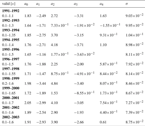
Table 1. CH4/HF reference relations from HALOE observations inside the vortex core: 1991–1992 to 2002–2003. Polynomial functions
of the form: [y]=Pn
i =0ai·[x]i with n≤4 are shown as well as the standard deviation of the observation points from the fitted reference
functionσ. valid [x] a0 a1 a2 a3 a4 σ 1991–1992 0.1–1.1 1.83 −2.49 2.72 −3.31 1.63 9.03×10⁻² 1992–1993 0.1–1.3 1.64 −1.71 7.33×10⁻¹ −1.91×10⁻² −1.55×10⁻¹ 9.95×10⁻² 1993–1994 0.1–1.35 1.85 −2.75 3.70 −3.15 9.31×10⁻¹ 1.04×10⁻¹ 1994–1995 0.1–1.4 1.76 −2.71 4.18 −3.71 1.10 8.98×10⁻² 1995–1996 0.1–1.5 1.65 −1.16 1.77×10⁻¹ −3.63×10⁻² 8.11×10⁻² 1996–1997 0.1–1.5 1.76 −1.88 2.25 −2.00 5.87×10⁻¹ 7.92×10⁻² 1997–1998 0.1–1.55 1.71 −1.47 8.75×10⁻¹ −4.91×10⁻¹ 8.44×10⁻² 8.14×10⁻² 1998–1999 0.2–1.6 1.98 −3.44 4.84 −3.40 8.07×10⁻¹ 8.46×10⁻² 1999–2000 0.1–1.65 1.72 −1.89 1.53 −8.55×10⁻¹ 1.73×10⁻¹ 8.67×10⁻² 2000–2001 0.1–1.7 2.05 −2.99 4.10 −3.05 7.54×10⁻¹ 7.27×10⁻² 2001–2002 0.1–1.6 1.89 −2.54 2.90 −1.93 4.40×10⁻¹ 7.39×10⁻² 2002–2003 0.1–1.6 1.91 −2.93 3.90 −2.66 0.61 8.75×10⁻²
and does not change significantly over the whole lifetime of the vortex in each year. In this study, a linear relationship of HALOE measurements was derived from profiles inside the polar vortex for each year, with a standard deviation of less than 0.1 ppmv (Table 1). Profiles deviating by more than
0.2 ppmv from the constant CH4/HF relation are neglected
in order to eliminate observations that are uncertain.
Besides CH4 and HF, the HALOE instrument measures
ozone and HCl, which are used as the active tracers in this study. HCl is chemically destroyed by heterogeneous reac-tions and increases due to the deactivation of chlorine via the reaction of Cl with CH4. Chemical ozone loss occurs if large
concentrations of chemically active halogen compounds are present in an air mass. This is the case in most years in late winter and spring inside the polar vortex in the presence of sunlight.
To derive chemical losses of ozone, first the ozone-tracer relation has to be determined at a time before ozone has chemically changed. This is usually the case in the early winter when rather little sunlight is present. The ozone-tracer relation, referred to as “early winter reference func-tion”, is mathematically formulated as a polynomial and is considered as the reference for chemically unperturbed
con-ditions. It is necessary to derive an early winter reference function for each of the twelve years considered to deter-mine chemical ozone loss for each year. The observation time of the underlying profiles considered has to be cho-sen carefully for this purpose. The turning point from sum-mer to winter circulation marks the time of the formation of the polar vortex. Thus, the time of the minimum of the ozone column density is the earliest time at which the early winter reference function can be determined. This point in time can be derived considering the total ozone column from global satellite measurements. Tilmes (2003, Sect. 3.3) used TOMS observations for this purpose. On the other hand, this time of the winter may not be the most suitable time to de-rive the early winter reference function if the early vortex is not yet strong enough. Horizontal mixing across the vortex edge may change the tracer-tracer relation without chemical changes. A case in point is the winter 1996–1997, where the ozone-tracer relation changed until the beginning of Jan-uary 1997, due to horizontal mixing processes (Tilmes et al., 2003b). Further, in winter 1991–1992 the ozone-tracer rela-tion changed from November 1991 to December 1991 due to mixing (see Sect. 3.1).
In summary, the early winter reference function has to be determined at a time when the vortex has already formed and, additionally, is sufficiently isolated from mid-latitude air, but at the same time early enough so that no ozone loss has yet taken place. Therefore, if the vortex is isolated, the reference function has to be derived as early as possible, if observa-tions are available. These condiobserva-tions are generally fulfilled for each of the derived reference functions and some excep-tions will be discussed in detail below.
To draw conclusions on possible chlorine activation and therefore possible ozone loss in a certain time period, the consideration of the value of “volume of possible PSC exis-tence”, VPSC, is useful because significant chlorine activation
is not possible without the existence of PSCs (e.g. Solomon, 1999). Additionally, here, the amount of solar illumination on the cold parts of the polar vortex is considered. Signifi-cant ozone loss is not possible without the existence of ac-tive chlorine components and further, without the presence of sunlight (e.g. Solomon, 1999).
VPSCdescribes the total volume on a certain potential
tem-perature level, where the temtem-perature (here determined from the UKMO analysis) does not exceed the PSC threshold tem-perature. This PSC threshold temperature was calculated
(Hanson and Mauersberger, 1988) for a HNO3 mixing
ra-tio of 10 ppbv and a H2O mixing ratio of 5 ppmv.
There-fore, if PSC existence is not possible at the time before the early winter reference function was derived, no chlorine ac-tivation and thus no ozone loss should have occurred. On the other hand, an existing potential for PSCs during the early winter may result in active chlorine components that cause
ozone loss if sunlight is present (see below). Using VPSC
as an indicator for chlorine activation, one has to keep in
mind that these calculations of VPSC do not include PSCs
which occur on the mesoscale due to orographically induced mountain waves (e.g. Fueglistaler et al., 2003). Further, the use of different meteorological analyses may result in differ-ences up to ≈25% of temperature analyses (Knudsen et al., 2002; Manney et al., 2003a) and therefore in differences in
the calculated VPSC. If HALOE measurements are available
at the time for which the early winter reference function is determined, chlorine activation can be clearly detected from the TRAC analysis of HCl-tracer correlations (M¨uller et al., 1996; Tilmes et al., 2003a) as a strong loss of HCl.
HALOE makes measurements fifteen times per day at each sunrise and sunset occultation along two latitude lines.
These lines move between 80◦N and 80◦S in about 45 days.
Therefore, measurements in high northern latitudes are avail-able every two or three months, depending on the year and in most of the years considered relatively few observations were available inside the early vortex. Thus, to derive the early winter reference function, additional data sources such as ILAS satellite measurements and balloon measurements were used.
For two out of twelve winters, for which no direct mea-surements could be obtained in the early vortex, a
methodol-ogy has been developed to estimate the early winter reference functions. In this way, for each of the twelve winters con-sidered a reliable early winter O3-tracer reference function
could be derived, as described below in Sect. 3.
A reliable calculation of ozone loss during the course of the winter is possible, as long as the polar vortex is iso-lated well enough so that the tracer-tracer correlation remains compact and unaltered in the absence of chemical changes. Tilmes et al. (2003b) and Tilmes (2003) have shown that a compact ozone-tracer correlation exists inside the polar vor-tex during January in the Arctic winter 1996–1997 when no chemical ozone loss is expected due to the lack of sunlight based on ILAS observations. The ILAS instrument measured seven months in high northern latitudes (58◦N–73◦N), thus providing good coverage of the polar vortex over this time period. Moreover, it was shown that the vortex has to be isolated well enough to obtain a compact reliable reference correlation. In the winter 1996–1997 this situation was found for the Arctic vortex since early January 1997. Further, dur-ing winter and sprdur-ing an exact criterion has to be defined to decide whether profiles are measured in or outside the vortex, because the characteristics of air outside the vortex are very different to vortex air. Using a mixture of profiles measured in and outside the vortex will lead to the erroneous conclu-sion that a compact ozone-tracer correlation does not exist.
Khosrawi et al. (2004) discussed the evolution of O3/N2O
of different isentropic levels based on ILAS measurements 1996–97. They did not separate isentropic levels at differ-ent altitudes into measuremdiffer-ents inside and outside the vortex and therefore did not obtain a compact January relationship,
whereas exactly the same data indicate a compact O3/N2O
correlation inside the vortex core if sorted according to the vortex criterion used here (Tilmes, 2003) (Fig. 4.4, the pole-ward edge of the vortex boundary region, using the algorithm derived by Nash et al., 1996).
In the study by Sankey and Shepherd (2003), the O3/CH4
correlation is considered in the course of an Arctic winter analysing results of the CMAM model. The ozone-tracer cor-relations from the model on the different isentropic levels are similar to those derived by Khosrawi et al. (2004) based on ILAS observations. Thus the shape of the lines should not be seen as a lack of compactness inside the polar vortex, as it is interpreted by Sankey and Shepherd (2003), but it is rather the result of considering measurements in high northern lati-tudes, which are not separated into profiles measured outside and inside the polar vortex.
Further, M¨uller et al. (2001) used balloon-borne measure-ments in the Arctic winter 1991–1992 to show that the im-pact of mixing between air masses from outside the vor-tex with air inside the vorvor-tex would result in a tendency to greater ozone mixing ratios in the ozone-tracer relation. Re-cent model calculations for the development of tracer distri-butions in the winter 1999/2000 (Konopka et al., 2003) cor-roborate this finding. The effect should thus lead to an under-estimation of the chemical ozone loss. Tilmes et al. (2003b),
using ILAS observations for winter 1996–1997, have shown that this effect is not significant after early January 1997. Even inside the vortex remnants in May 1997, a compact cor-relation is found.
In this study we argue that a compact correlation exists during all the observed twelve Arctic winters. Especially, the analysis of the very warm winters (1998–1999 and 2001– 2002) – where no substantial chemical ozone loss is expected – demonstrates that the ozone-tracer correlations do not sig-nificantly change due to mixing processes, although the vor-tices are less strong compared to other winters. Only if the vortex completely breaks down and reforms, as was the case in March 2001, is it impossible to obtain reliable results us-ing the TRAC technique.
2.2 Error analysis
An error analysis was performed consistently for all the years analysed here. In the early winter and during the course of the winter, the scatter of the ozone-tracer relations arises, on the one hand, due to variability of the mixing ratios of tracers inside the vortex, and, on the other hand, it may possibly be due to the random error of the satellite measurements. Both these uncertainties are estimated by calculating the standard deviation of the profiles contributing to the early winter ref-erence function.
Further, no systematic error of the satellite measurements is taken into account because assuming that all available measurements of one satellite are affected in the same way it would have no impact on the ozone loss calculation. There-fore, the uncertainty of results was derived from the uncer-tainty of the early winter reference function. Additionally, the standard deviation of monthly averaged column ozone loss deduced from the individual profiles is considered. This describes the homogeneity of the deduced ozone loss during a particular time span and in a particular region. Inhomo-geneities may be caused by both the inhomogeneity of the ozone loss inside the vortex and the random error of the satel-lite measurements, as described above.
Mixing processes may change the early winter reference function without chemical change if the vortex is not
iso-lated. However, a significant increase in the uncertainty
range due to mixing processes in the early vortex is not ex-pected, because each profile used to derive an early win-ter reference function was located poleward of the vortex edge (using the Nash criterion). The vortex was isolated for most years considered at the time when the reference func-tion was derived. This can be assumed regarding the evo-lution of calculated PV values at the vortex edge using the Nash criterion. At the time when the reference function was derived, PV values at the vortex edge are 30–35 PV units (1PVU=10−6K m2/(kg s)) at the 475 K level for all year. In the following two weeks, PV values increase in the most of the years at the 475 K level (except for the winter 1998– 1999). Therefore, the uncertainty due to dynamics on the
reference function should be small in all the years consid-ered. In 1998–1999 the vortex was less strong although still isolated; in this winter, a stronger influence of mixing on the early vortex reference cannot be excluded.
The impact of mixing processes during the entire winter period of the years considered should be small for the same reason. Only in the middle of February 2001 did the vortex break down completely. Therefore, no ozone loss is calcu-lated after this event. In 1991–1992, a major warming at the end of January may have impacted the tracer-tracer correla-tions leading to an underestimation of chemical ozone loss in this year (see Sect. 2.1). Therefore, the derived value of ozone loss for this winter constitutes a lower limit. Further, results of the winter 1997–1998 and 2000–2001 had to be de-rived using a reference function based on climatology values and are thus more uncertain compared to results derived from a reference function based directly on measurements of the specific year. Nevertheless, these reference functions are the average of all the de-trended early winter reference functions and should therefore be reliable within the reported range of uncertainty.
To derive results with minimum uncertainty, it is also necessary to calculate ozone loss in the appropriate altitude range. Column ozone loss is therefore calculated for an al-titude range of 380–550 K, 400–500 K and 40–100 hPa (to compare the results with other studies) from HALOE obser-vations, because within this range the empirical ozone-tracer reference relations are valid and possible mixing processes below 380 K are excluded. The smallest uncertainty arises if the column ozone loss is calculated in an altitude range between 400–500 K. Here, the vortex is most compact and accuracies of satellite data are better than at lower altitudes.
3 Impact of meteorological conditions on ozone-tracer and HCl-tracer relations
3.1 Development of early winter reference functions
The early winter reference function is derived individually from all available HALOE measurements inside the early vortex for the six winters 1992–1993 to 1995–1996 and in 1998–1999 and 2001–2002. The profiles used were located inside the early vortex for each year, at a time when in general no ozone loss was expected (as outlined below). For 1991– 1992 (M¨uller et al., 2001), 1999–2000 (M¨uller et al., 2002) and 2002–2003 (Tilmes et al., 2003a), early winter reference functions were derived from balloon observations. In winter 1996–1997, ILAS observations were used to define an early winter reference function to calculate ozone loss from mea-surements made by HALOE in late winter and spring (Tilmes et al., 2003b).
An overview of the mathematically formulated tracer-tracer early winter reference functions derived only from HALOE observations inside the early vortex is summarised
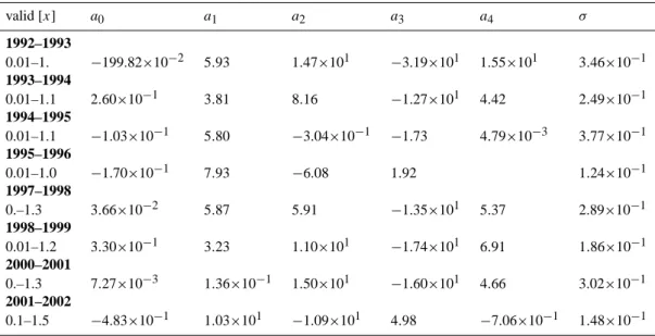
Table 2. O3/HF reference relations from HALOE observations: 1992–1993 to 2001–2002 (see text). Polynomial functions of the form:
[y]=Pn
i =0ai·[x]iwith n≤4 are shown as well as the standard deviation of the observation points from the fitted reference functionσ .
valid [x] a0 a1 a2 a3 a4 σ 1992–1993 0.01–1. −199.82×10⁻² 5.93 1.47×101 −3.19×101 1.55×101 3.46×10⁻¹ 1993–1994 0.01–1.1 2.60×10⁻¹ 3.81 8.16 −1.27×101 4.42 2.49×10⁻¹ 1994–1995 0.01–1.1 −1.03×10⁻¹ 5.80 −3.04×10⁻¹ −1.73 4.79×10⁻³ 3.77×10⁻¹ 1995–1996 0.01–1.0 −1.70×10⁻¹ 7.93 −6.08 1.92 1.24×10⁻¹ 1997–1998 0.–1.3 3.66×10⁻² 5.87 5.91 −1.35×101 5.37 2.89×10⁻¹ 1998–1999 0.01–1.2 3.30×10⁻¹ 3.23 1.10×101 −1.74×101 6.91 1.86×10⁻¹ 2000–2001 0.–1.3 7.27×10⁻³ 1.36×10⁻¹ 1.50×101 −1.60×101 4.66 3.02×10⁻¹ 2001–2002 0.1–1.5 −4.83×10⁻¹ 1.03×101 −1.09×101 4.98 −7.06×10⁻¹ 1.48×10⁻¹
Table 3. O3/CH4reference relations from HALOE observations: 1992–1993 to 2001–2002 (see text). Polynomial functions of the form:
[y]=Pn
i =0ai·[x]iwith n≤4 are shown as well as the standard deviation of the observation points from the fitted reference functionσ .
valid [x] a0 a1 a2 a3 a4 σ 1992–1993 0.45–1.65 8.77 −2.39×101 4.51×101 −3.59×101 9.34 2.31×10⁻¹ 1993–1994 0.4–1.7 4.72 −6.55 1.73×101 −1.75×101 5.12 3.09×10⁻¹ 1994–1995 0.45–1.6 4.19 −3.51 1.14×101 −1.38×101 4.44 3.56×10⁻¹ 1995–1996 0.6–1.7 −2.98 2.55×101 −3.00×101 1.24×101 −1.68 3.09×10⁻¹ 1997–1998 0.6–1.7 3.70 −2.09 1.00×101 −1.19×101 3.55 4.40×10⁻¹ 1998–1999 0.6–1.7 4.55×10⁻¹ 1.27×101 −1.27×101 3.11 1.04524×10⁻¹ 2000–2001 0.6–1.7 5.00 −8.95 2.14×101 −1.92×101 5.16 4.43×10⁻¹ 2001–2002 0.6–1.7 4.49 −6.35 1.36×101 −1.26×101 3.55 1.85×10⁻¹
in Tables 2 and 3. As in Table 1, polynomial functions of the
form: [y]=Pn
i =0ai·[x]i with n≤4 are reported as well as
the standard deviationσ of the observation points from the
fitted reference function. The empirical relations are valid for
mixing ratios of CH4in ppmv, HF in ppbv and O3in ppmv,
respectively.
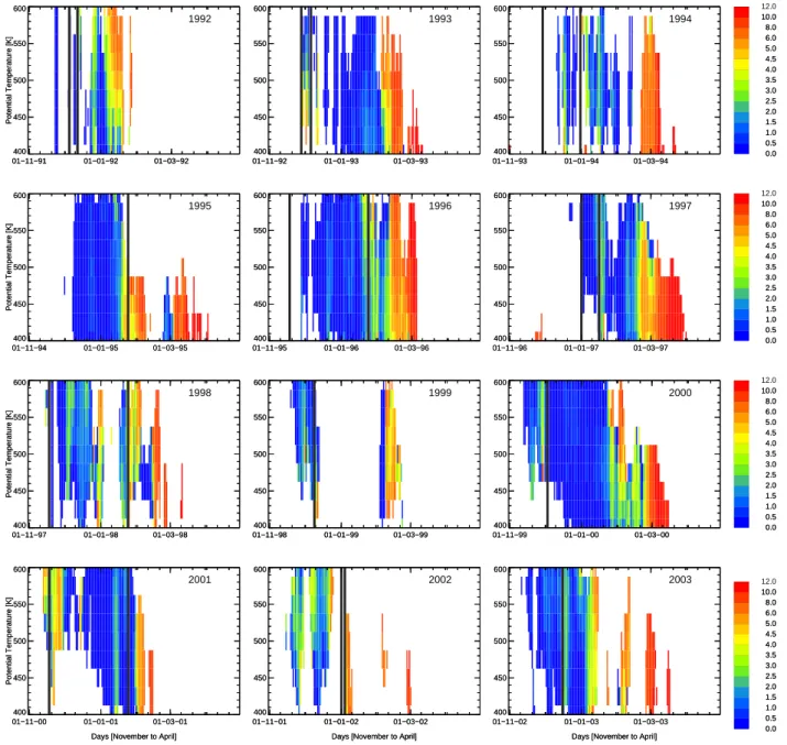
The time (interval) at which the early winter reference functions were derive in each year is shown in Fig. 1 by ver-tical black lines. In 1998–1999 and 2000–2001, the HALOE
climatology was used to derive the early winter reference function. Therefore, the time interval between the earliest date of all profiles used and latest date of all profiles used in these years is shown. This figure shows daily sun hours at possible PSC areas for all the twelve years considered. It indicates, on the one hand, wether PSC existence is pos-sible at the time when the early winter reference function was derived and, further, how strongly these PSC areas were illuminated before the early winter reference function was
400 450 500 550 600 Potential Temperature [K] 400 450 500 550 600 Potential Temperature [K] 01−11−91 01−01−92 01−03−92 01−11−91 01−01−92 01−03−92 1992 400 450 500 550 600 400 450 500 550 600 01−11−92 01−01−93 01−03−93 01−11−92 01−01−93 01−03−93 1993 400 450 500 550 600 400 450 500 550 600 01−11−93 01−01−94 01−03−94 01−11−93 01−01−94 01−03−94 1994 0.0 0.5 1.0 1.5 2.0 2.5 3.0 3.5 4.0 4.5 5.0 6.0 8.0 10.0 0.0 0.5 1.0 1.5 2.0 2.5 3.0 3.5 4.0 4.5 5.0 6.0 8.0 10.0 12.0 400 450 500 550 600 Potential Temperature [K] 400 450 500 550 600 Potential Temperature [K] 01−11−94 01−01−95 01−03−95 01−11−94 01−01−95 01−03−95 1995 400 450 500 550 600 400 450 500 550 600 01−11−95 01−01−96 01−03−96 01−11−95 01−01−96 01−03−96 1996 400 450 500 550 600 400 450 500 550 600 01−11−96 01−01−97 01−03−97 01−11−96 01−01−97 01−03−97 1997 0.0 0.5 1.0 1.5 2.0 2.5 3.0 3.5 4.0 4.5 5.0 6.0 8.0 10.0 0.0 0.5 1.0 1.5 2.0 2.5 3.0 3.5 4.0 4.5 5.0 6.0 8.0 10.0 12.0 400 450 500 550 600 Potential Temperature [K] 400 450 500 550 600 Potential Temperature [K] 01−11−97 01−01−98 01−03−98 01−11−97 01−01−98 01−03−98 1998 400 450 500 550 600 400 450 500 550 600 01−11−98 01−01−99 01−03−99 01−11−98 01−01−99 01−03−99 1999 400 450 500 550 600 400 450 500 550 600 01−11−99 01−01−00 01−03−00 01−11−99 01−01−00 01−03−00 2000 0.0 0.5 1.0 1.5 2.0 2.5 3.0 3.5 4.0 4.5 5.0 6.0 8.0 10.0 0.0 0.5 1.0 1.5 2.0 2.5 3.0 3.5 4.0 4.5 5.0 6.0 8.0 10.0 12.0 400 450 500 550 600 Potential Temperature [K] 400 450 500 550 600 Potential Temperature [K] 01−11−00 01−01−01 01−03−01 Days [November to April] 01−11−00 01−01−01 01−03−01
Days [November to April]
2001 400 450 500 550 600 400 450 500 550 600 01−11−01 01−01−02 01−03−02 Days [November to April] 01−11−01 01−01−02 01−03−02
Days [November to April]
2002 400 450 500 550 600 400 450 500 550 600 01−11−02 01−01−03 01−03−03 Days [November to April] 01−11−02 01−01−03 01−03−03
Days [November to April]
2003 0.0 0.5 1.0 1.5 2.0 2.5 3.0 3.5 4.0 4.5 5.0 6.0 8.0 10.0 0.0 0.5 1.0 1.5 2.0 2.5 3.0 3.5 4.0 4.5 5.0 6.0 8.0 10.0 12.0
Fig. 1. Daily sun hours at possible PSC areas over the entire polar vortex, as a function of altitude, are shown for the period from November to April for the twelve winters between 1991–92 and 2002–2003. White area indicates regions where the area of possible PSC existence is zero. Black lines indicate the time (interval) for which the early winter reference function was derived.
calculated. In this way, we can estimate if some ozone loss may have occurred before the early winter reference function was derived, because the existence of PSCs and solar radia-tion are responsible for ozone loss.
As an example, the derivation of the early winter refer-ence function in 1995–1996 from HALOE profiles inside the early vortex is discussed. In this winter, HALOE vortex pro-files were available at the end of November. At this time of
the winter, the VPSC was negligible. No deviation from the
unperturbed HCl/HF relation was found. Therefore, no ac-tivated chlorine compounds and thus no ozone loss can be
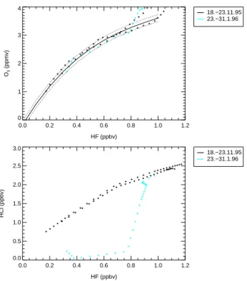
expected. Two months later, at the end of January (Fig. 2, bottom panel), one profile inside the vortex boundary region indicates strong chlorine activation noticeable as a change
in the HCl/HF relation corresponding to a large VPSC
dur-ing January. But still no changes in the O3/HF relation are
detected (Fig. 2, top panel). Changes in the O3/HF relation
due to isentropic mixing are not expected during December and January, because at that time the vortex was already very
strong. Further, at this time and location (≈50◦N) of the
profile solar illumination is expected, but the vortex was il-luminated only for a very short time before 23–31 January
0.0 0.2 0.4 0.6 0.8 1.0 1.2 HF (ppbv) 0 1 2 3 4 O3 (ppmv) 18.−23.11.95 23.−31.1.96 0.0 0.2 0.4 0.6 0.8 1.0 1.2 HF (ppbv) 0.0 0.5 1.0 1.5 2.0 2.5 3.0 HCl (ppbv) 18.−23.11.95 23.−31.1.96
Fig. 2. Tracer-tracer profiles inside the outer early vortex of the year 1995–1996 from HALOE measurements with HF as the pas-sive tracer. In the top panel, the chemical active tracer is O3and in
the bottom panel the chemical active tracer is HCl. The early winter reference function for the O3/HF relation 1995–1996, top panel, is
indicated as a black solid line and the uncertainty of the reference function is represented by black dotted lines.
1996 (see Fig. 1). Therefore, the HCl was already strongly reduced although little ozone loss inside the range of uncer-tainty of the reference function was found. Of course, the
HCl-tracer relation changes much faster than the O3-tracer
relation, because chlorine activation occurs on much shorter time scales than ozone loss. The fact that in 1996 – in spite of the early vortex having been cold and strong – no signifi-cant ozone loss occurred during January may be explained by the very small amount of sunlight that illuminated the early vortex.
In the following, the derivation of the early winter ref-erence function from balloon observations in 1991–1992, 1999–2000 and 2002–2003 is briefly described. Thereafter, early winter reference functions of the other years considered are discussed. For winter 1991–1992, the early winter refer-ence function was derived from measurements of ozone and
N2O made by cryosampler measurements (Schmidt et al.,
1987) on 5 and 12 December 1991, respectively. At this
time, a small VPSC was calculated, but these VPSC are not
illuminated (see Fig. 1) and therefore no ozone loss can be expected before this time.
The O3/N2O profiles were transformed to O3/CH4with the
N2O/CH4relationship from Engel et al. (1996), see M¨uller
6−Nov−1991 to 14−Jan−1992 0.4 0.6 0.8 1.0 1.2 1.4 1.6 CH4 (ppmv) 0 1 2 3 4 5 O3 (ppmv) Kiruna Balloons 5.12.91 Kiruna Balloons 12.12.91 Kiruna Balloons 5.12.91 Kiruna Balloons 12.12.91
Fig. 3. The early winter reference function 1991–1992, shown as a black line, was derived from balloon measurements from December 1991 (coloured symbols). Dotted lines indicate the range of uncer-tainty in the reference function. Observations made by HALOE within the vortex in November 1991 (black plus signs) and in Jan-uary (black squares) are also shown.
et al. (2001). To derive the O3/HF reference function, the
O3/CH4 relation was converted using the CH4/HF relation
derived from HALOE observations for the winter 1991–1992 (Table 1).
The vortex started forming in November 1991. One
HALOE profile was found inside the early vortex at the be-ginning of November, with low ozone mixing ratios com-pared to profiles inside the vortex measured in January (see Fig. 3, black plus signs). At that time the vortex was not well developed and mixing in of air masses from outside the vortex was still possible. Therefore, the low ozone mixing ratios observed in November increased until the vortex be-came fully isolated in December. The HALOE profiles in January 1992 scatter below the derived reference relation by
about 1.2 ppmv CH4level (see Fig. 3). Thus ozone loss had
already occurred during January 1992, in accordance with a relatively small, but illuminated volume of possible PSC existence in the first two weeks of January (see Figs. 1 and 8). In contrast to the winter 1995–1996, ozone loss during
January 1992 was much stronger although VPSC in January
1996 was even larger than in January 1991–1992. However,
VPSCwere much less illuminated in January 1996 compared
to January 1992 (see Fig. 1). This shows that ozone loss is influenced by solar radiation in addition to VPSC, as further
discussed in Sect. 6.
In winter 1999–2000, again no HALOE observations were available inside the early vortex to derive the early winter ref-erence function. Fortunately, during the SOLVE-THESEO 2000 campaign two balloon flights have been conducted in-side the early vortex, the OMS (Observations of the Middle
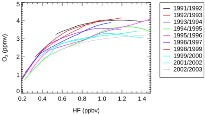
0.2 0.4 0.6 0.8 1.0 1.2 HF (ppbv) 0 1 2 3 4 5 O3 (ppmv) 1991/1992 1992/1993 1993/1994 1994/1995 1995/1996 1996/1997 1998/1999 1999/2000 2001/2002 2002/2003 0.4 0.6 0.8 1.0 1.2 1.4 1.6 CH4 (ppmv) 0 1 2 3 4 5 O3 (ppmv) 1991/1992 1992/1993 1993/1994 1994/1995 1995/1996 1996/1997 1998/1999 1999/2000 2001/2002 2002/2003
Fig. 4. Early winter reference relations for the ten years from 1991– 1992 to 2002–2003 are indicated as coloured lines. O3/HF is shown
in the top panel and O3/CH4is shown in the bottom panel.
Stratosphere) in-situ flight on 19 November 1999 and the OMS remote flight on 3 December 1999 (e.g. M¨uller et al., 2002). HF measurements were only available from the MkIV instrument on the OMS-remote flight. Thus, these data were
used to derive the O3/HF reference function for this
win-ter. Two early winter reference functions were derived using CH4as the long-lived tracer, one was derived using the
OMS-in-situ measurements and the second using the OMS-remote flight measurements (M¨uller et al., 2002). Only a little ozone loss may have already occurred on 3 December 1999 because of small VPSCthat is slightly illuminated (see Fig. 1).
For 2002–2003, MkIV balloon observations in mid-December 2002 (Toon et al., 1999) were used to derive the early winter reference function (Tilmes et al., 2003a). The early winter reference functions of the winters 2002–2003 were derived from measurements at a time when the vortex had already developed. Before this time, a large volume of PSCs had already been detected and some activation of chlo-rine had already occurred in altitudes above 500 K (Tilmes et al., 2003a). However, hardly any illumination of the PSC area was detected and no significant ozone loss can be ex-pected before the time when the reference function was de-rived.
In winters 1992–1993, 1993–1994, 1995–1996 and 1996– 1997, the early winter reference functions were derived in a
0.2 0.4 0.6 0.8 1.0 1.2 1.4 HF (ppbv) 0 1 2 3 4 5 O3 (ppmv) 1991/1992 1992/1993 1993/1994 1994/1995 1995/1996 1996/1997 1998/1999 1999/2000 2001/2002 2002/2003 Thu Jun 24 11:16:17 2004 imone/IDL/HALOE_PRO/haloe_intern_set_plot.pro HF_SCATTER/haloe_hf_references_detr.ps
Fig. 5. Early winter reference relations for ten years from 1991–
1992 to 2002–2003 are indicated as coloured lines. O3/HF is
shown; HF being corrected for the growth rate of HF derived from the HALOE CH4/HF relationship for each year (Tilmes, 2003).
certain time interval (see Fig. 1). At the beginning of this time interval, no ozone loss is expected because PSCs were detected (see Fig. 1). At the end of this time interval, the analysis does not show any ozone loss. However, only pro-files inside the outer vortex are considered for most of this year to derive the early winter reference function, so we can-not prove wether ozone loss had already occurred inside the vortex core.
HALOE measurements in January 1994–1995 show
strong deviations of the HCl/HF relations at the time when
the reference function was deduced. A strong volume of PSCs was calculated before that time, and some illumina-tion of the PSCs was detected. Rex et al. (2003a) and Goutail et al. (1999) reported large ozone loss rates for January 1995. These losses may have already resulted in a small decrease of ozone in the O3/HF relation before the time when the
ref-erence function was deduced. Therefore, these ozone losses cannot be included in the calculations below. As in 1994– 1995, in winter 2001–2002 some ozone loss may have oc-curred at the time when the reference function was derived.
However, VPSCwas much smaller in early 2001–2002. The
derived ozone-tracer early winter reference functions for ten out of twelve years are shown in Fig. 4.
The deduced ozone-tracer relation in the early winter has its own characteristics each year. This is due to inter-annual differences in polar vortex development and not due to chem-ical loss (Manney et al., 2003b). Considering ozone-tracer relations, year by year variations are expected to be influ-enced by a trend of mixing ratios of the long-lived tracer used. This is the case using HF as the long-lived tracer (Fig. 4, top panel), because HF mixing ratios increased by
≈0.4 ppbv in the middle stratosphere from 1991 to 2000
(Tilmes, 2003).
On the other hand, the growth rate of 60 ppbv in 12
years of CH4– taken from the tropospheric growth rate
de-rived by Simpson et al. (2002) – is very small compared
0.5–1.5 ppmv) and therefore is not significant for the present analysis. Further, ozone was relatively constant during the 1990s in northern mid-latitudes (WMO, 2003). Neverthe-less, a decrease of ozone was found in the polar regions, but mainly in the southern hemisphere (WMO, 2003). Therefore,
considering O3/CH4 reference functions (Fig. 4, bottom
panel) the interannual differences of the early winter ref-erence functions are not a result of a significant trend of methane. In this study, we obtain some indications of a trend of ozone in high northern altitudes towards lower ozone mix-ing ratios, but interannual differences in ozone mixmix-ing ra-tios are possible for different reasons (as described below). O3/HF early winter reference functions can be de-trended
with regard to HF, using the HF growth rate deduced from
the HALOE HF/CH4relationships (Table 1) (Tilmes, 2003).
The range of interannual differences of ≈1 ppmv ozone mixing ratio – in altitudes above the 0.8 ppbv level of HF
or the 1.0 ppmv level of CH4 – are similar for both O3/HF
and O3/CH4relationships (see Figs. 4, bottom panel and 5).
The largest ozone mixing ratios are found in winter 1991– 1992. This is possibly due to enhanced global transport in this winter owing to the eruption of Pinatubo in June 1991. Very small ozone mixing ratios are found for the three win-ters 1999–2000, 2001–2002 and 2002–2003. This may be due to an earlier isolation of the polar vortex, for example in winter 2002–2003. Additionally, ozone loss may have al-ready occurred at the time when the reference function was derived in winter 1999–2000 and 2001–2002 (see Fig. 1). Due to the different influences that control ozone mixing ra-tios in high northern latitudes in the early winter, a possible trend of ozone cannot be determined in this study.
Thus, it is not possible to use one single reference function for all years. For the winter 1997–1998 and 2000–2001, nei-ther HALOE nor any onei-ther measurements were obtained in the early vortex. Therefore, the early winter reference func-tions of these years were constructed from a climatology of all HALOE profiles measured inside the early vortex over the ten year period between 1992 and 2002. Actually, mea-surements inside the early vortex are available for six win-ters (1992–1993, 1993–1994, 1994–1995, 1995-1996, 1998–
1999 and 2001–2002). The HALOE O3/HF and O3/CH4
profiles are corrected for the growth rate of HF and CH4,
respectively, between each single year and the year 1997–
1998 (2000–2001). The CH4 growth was taken from the
tropospheric growth rate (Simpson et al., 2002). The HF
growth rate was deduced from the HALOE HF/CH4
rela-tionships (Table 1) (Tilmes, 2003). No correction was ap-plied to ozone, as described above. Thus, for winters 1997– 1998 and 2000–2001 in each case two early winter reference relations were derived, one using HF as the long-lived tracer
and one using CH4(Tables 2 and 3).
3.2 The evolution of tracer-tracer relations during twelve
Arctic winters
Active chlorine inside the polar vortex causes chemical ozone loss in the presence of sunlight. Chlorine activation in the Arctic lower stratosphere may be identified as a strong re-duction of HCl compared to normal values. Therefore, using measurements made by HALOE, the evolution of the chlo-rine chemistry can be inferred from the development of the tracer relation during each year. The evolution of HCl-tracer relation and O3-tracer relation is analysed for each of
the twelve observed winter periods (Figs. 6 and 7). Low temperatures in the polar vortex cause the formation of PSC and thus control the activation of chlorine and consequently the chemical destruction of ozone. If temperatures are suffi-ciently low PSCs occur in the polar stratosphere. Therefore,
VPSC is used here to analyse the interaction between
mete-orological conditions and development of tracer-tracer rela-tionships for each winter (Fig. 8). Further, a division into cold, moderately cold and warm winters is carried out at the end of this section. Additionally, a measure of the strength of the vortex is determined.
– 1991–1992:
The cold vortex in winter 1991–1992 was disturbed by several warming pulses between November and Febru-ary (Naujokat et al., 1992). The threshold temperature for PSCs was only reached during January. Therefore, significant ozone depletion can be expected starting in January 1992. At the end of January, a major warming resulted in transport of air into the vortex (e.g. Grooß et al., 2003). However, the vortex in the lower
strato-sphere was not much affected. The zonal winds at 60◦N
considerably weakened, but remained westerly (Nau-jokat et al., 1992). In the second part of March and April 1992, ozone loss was found to be homogeneous in the Arctic vortex. This is an indication that the air from outside that entered the vortex at the end of January was well mixed within the vortex during March and April. During March, the temperatures at the North Pole steadily increased and the vortex finally broke down at the end of April (Naujokat et al., 1992). In January, February and at the beginning of March, very low HCl mixing ratios are clearly noticeable and strong chlorine activation (Fig. 6) occurred in the lower stratosphere. HCl mixing ratios are nearly zero in January and less than 0.3 ppbv in February below the 0.6 ppbv HF level, which is below the 420 K potential temperature level. By April, the HCl levels increased towards unperturbed values, especially at altitudes below ≈420 K. The vortex became steadily weaker during April. From February up to the beginning of April a moderate homogeneous
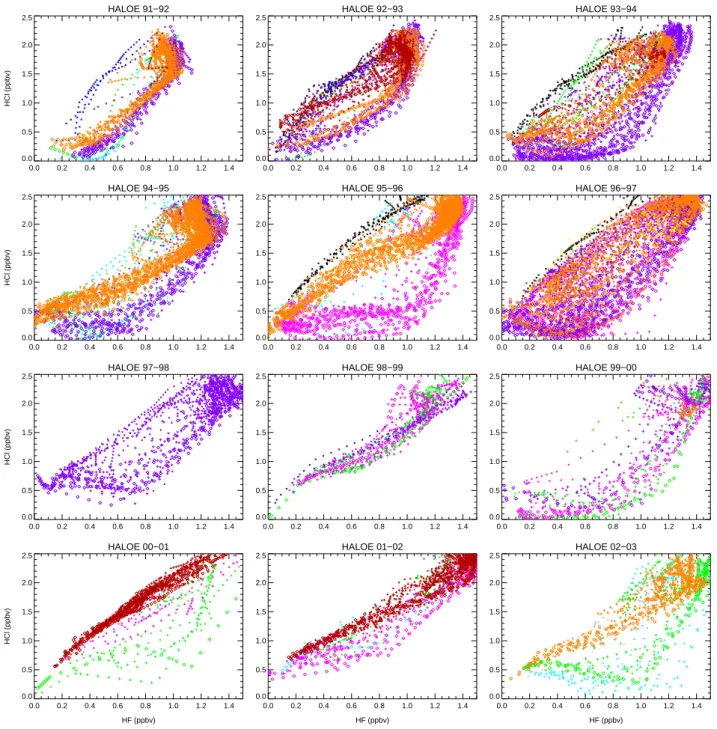
HALOE 91−92 0.0 0.2 0.4 0.6 0.8 1.0 1.2 1.4 0.0 0.5 1.0 1.5 2.0 2.5 HCl (ppbv) HALOE 92−93 0.0 0.2 0.4 0.6 0.8 1.0 1.2 1.4 0.0 0.5 1.0 1.5 2.0 2.5 HALOE 93−94 0.0 0.2 0.4 0.6 0.8 1.0 1.2 1.4 0.0 0.5 1.0 1.5 2.0 2.5 HALOE 94−95 0.0 0.2 0.4 0.6 0.8 1.0 1.2 1.4 0.0 0.5 1.0 1.5 2.0 2.5 HCl (ppbv) HALOE 95−96 0.0 0.2 0.4 0.6 0.8 1.0 1.2 1.4 0.0 0.5 1.0 1.5 2.0 2.5 HALOE 96−97 0.0 0.2 0.4 0.6 0.8 1.0 1.2 1.4 0.0 0.5 1.0 1.5 2.0 2.5 HALOE 97−98 0.0 0.2 0.4 0.6 0.8 1.0 1.2 1.4 0.0 0.5 1.0 1.5 2.0 2.5 HCl (ppbv) HALOE 98−99 0.0 0.2 0.4 0.6 0.8 1.0 1.2 1.4 0.0 0.5 1.0 1.5 2.0 2.5 HALOE 99−00 0.0 0.2 0.4 0.6 0.8 1.0 1.2 1.4 0.0 0.5 1.0 1.5 2.0 2.5 HALOE 00−01 0.0 0.2 0.4 0.6 0.8 1.0 1.2 1.4 HF (ppbv) 0.0 0.5 1.0 1.5 2.0 2.5 HCl (ppbv) HALOE 01−02 0.0 0.2 0.4 0.6 0.8 1.0 1.2 1.4 HF (ppbv) 0.0 0.5 1.0 1.5 2.0 2.5 HALOE 02−03 0.0 0.2 0.4 0.6 0.8 1.0 1.2 1.4 HF (ppbv) 0.0 0.5 1.0 1.5 2.0 2.5
Fig. 6. HCl/HF relations are shown for the twelve winters between 1991–1992 and 2002–2003 as measured from profiles inside the vortex core (diamonds), inside the outer vortex (large plus signs), and inside an outer part of the outer vortex (small crosses) by HALOE. Different colours of profiles indicate the different time intervals when profiles were observed: November (black), December (blue), January (cyan), February (green), first part of March (magenta), second part of March (purple), first part of April (orange), second part of April (dark red).
– 1992–1993:
The vortex in winter 1992–1993 was cold and nearly
undisturbed until the end of January. A strong
mi-nor warming in February shifted the cold air (with
low ozone values) towards Europe. This, together
with a blocking anticyclone in the troposphere, led to low total ozone values over Europe in February
(Nau-jokat and Labitzke, 1993). Conditions for chemical
ozone loss were reached because of the low strato-spheric temperatures (Fig. 8). Unfortunately, no mea-surements were taken inside the vortex in February, but HCl measurements inside the outer part of the vor-tex boundary region indicate a strong chlorine activa-tion in February at lower altitudes (Fig. 6, small green
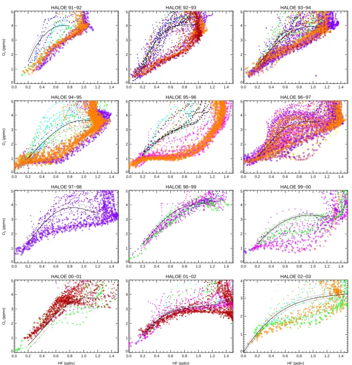
HALOE 91−92 0.0 0.2 0.4 0.6 0.8 1.0 1.2 1.4 0 1 2 3 4 5 O3 (ppmv) HALOE 92−93 0.0 0.2 0.4 0.6 0.8 1.0 1.2 1.4 0 1 2 3 4 5 HALOE 93−94 0.0 0.2 0.4 0.6 0.8 1.0 1.2 1.4 0 1 2 3 4 5 HALOE 94−95 0.0 0.2 0.4 0.6 0.8 1.0 1.2 1.4 0 1 2 3 4 5 O3 (ppmv) HALOE 95−96 0.0 0.2 0.4 0.6 0.8 1.0 1.2 1.4 0 1 2 3 4 5 HALOE 96−97 0.0 0.2 0.4 0.6 0.8 1.0 1.2 1.4 0 1 2 3 4 5 HALOE 97−98 0.0 0.2 0.4 0.6 0.8 1.0 1.2 1.4 0 1 2 3 4 5 O3 (ppmv) HALOE 98−99 0.0 0.2 0.4 0.6 0.8 1.0 1.2 1.4 0 1 2 3 4 5 HALOE 99−00 0.0 0.2 0.4 0.6 0.8 1.0 1.2 1.4 0 1 2 3 4 5 HALOE 00−01 0.0 0.2 0.4 0.6 0.8 1.0 1.2 1.4 HF (ppbv) 0 1 2 3 4 5 O3 (ppmv) HALOE 01−02 0.0 0.2 0.4 0.6 0.8 1.0 1.2 1.4 HF (ppbv) 0 1 2 3 4 5 HALOE 02−03 0.0 0.2 0.4 0.6 0.8 1.0 1.2 1.4 HF (ppbv) 0 1 2 3 4
Fig. 7. As Fig. 6 but O3/HF relations.
crosses). Temperatures started rising in March and the final break-up of the vortex occurred around 10 April. At that time HCl levels recovered to unperturbed values. Strong (homogeneous) deviation from the O3-tracer
ref-erence function is obvious in March and April (Fig. 7).
Until the end of April, the deviation from the O3/HF
reference function did not further change inside the re-maining parts of the vortex.
– 1993–1994:
The early vortex in winter 1993–1994 was slightly dis-turbed in November, December and January (Naujokat et al., 1995a). Owing to the warming over Europe in February, the vortex was split most of the time. At the end of February and the beginning of March, the vortex air masses cooled down again and temperatures were below the threshold for the existence of PSCs for a few days (Fig. 8). A small decrease of HCl in February is
350 400 450 500 550 600 Potential Temperature [K] 350 400 450 500 550 600 Potential Temperature [K] 01−11−91 01−01−92 01−03−92 1992 350 400 450 500 550 600 350 400 450 500 550 600 01−11−92 01−01−93 01−03−93 1993 350 400 450 500 550 600 350 400 450 500 550 600 01−11−93 01−01−94 01−03−94 −1.0 0.0 0.1 1.0 2.5 5.0 7.5 10.0 12.5 15.0 17.5 20.0 1994 350 400 450 500 550 600 Potential Temperature [K] 350 400 450 500 550 600 Potential Temperature [K] 01−11−94 01−01−95 01−03−95 1995 350 400 450 500 550 600 350 400 450 500 550 600 01−11−95 01−01−96 01−03−96 1996 350 400 450 500 550 600 350 400 450 500 550 600 01−11−96 01−01−97 01−03−97 −1.0 0.0 0.1 1.0 2.5 5.0 7.5 10.0 12.5 15.0 17.5 20.0 1997 350 400 450 500 550 600 Potential Temperature [K] 350 400 450 500 550 600 Potential Temperature [K] 01−11−97 01−01−98 01−03−98 1998 350 400 450 500 550 600 350 400 450 500 550 600 01−11−98 01−01−99 01−03−99 1999 350 400 450 500 550 600 350 400 450 500 550 600 01−11−99 01−01−00 01−03−00 −1.0 0.0 0.1 1.0 2.5 5.0 7.5 10.0 12.5 15.0 17.5 20.0 2000 350 400 450 500 550 600 Potential Temperature [K] 350 400 450 500 550 600 Potential Temperature [K] 01−11−00 01−01−01 01−03−01 Days [November to April]
2001 350 400 450 500 550 600 350 400 450 500 550 600 01−11−01 01−01−02 01−03−02 Days [November to April]
2002 350 400 450 500 550 600 350 400 450 500 550 600 01−11−02 01−01−03 01−03−03 Days (November to April)
−1.0 0.0 0.1 1.0 2.5 5.0 7.5 10.0 12.5 15.0 17.5 20.0 2003
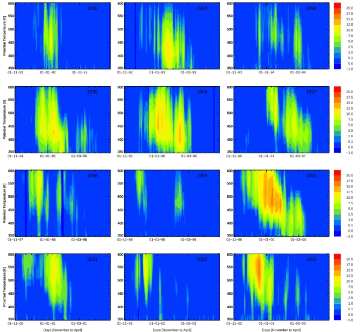
Fig. 8. The volume of possible PSC existence in 106km2over the entire polar vortex, as a function of altitude, is shown for the period from November to April for the twelve winters between 1991–1992 and 2002–2003. The PSC threshold temperature was calculated with the analysed UKMO temperatures and pressures assuming typical stratospheric mixing ratios of HNO3(10 ppbv) and H2O (5 ppmv) (Hanson and Mauersberger, 1988).
noticeable from the HCl/HF relation (Fig. 6).
After-wards HCl strongly decreased during March (HCl mix-ing ratios were below 0.1 ppbv for HF mixmix-ing ratios below 0.7 ppbv). During April the HCl levels quickly increased while the vortex became weaker. In March
and April moderate deviations from the O3/HF
refer-ence function became noticeable (Fig. 6), although the chlorine activation in March seemed to be rather pro-nounced.
– 1994–1995:
The vortex in 1994–1995 formed early and was very cold and strong especially between mid-December and
mid-January. A large VPSCwas deduced for the whole
of January 1995. Owing to a warming event in Febru-ary the vortex was displaced towards Siberia but did not break. The temperatures of the cold centre of the vor-tex towards Siberia were low enough for PSC forma-tion until 10 February (Naujokat et al., 1995b). Record low temperatures were reached again in the lower strato-sphere in March (Naujokat et al., 1995b). In April the
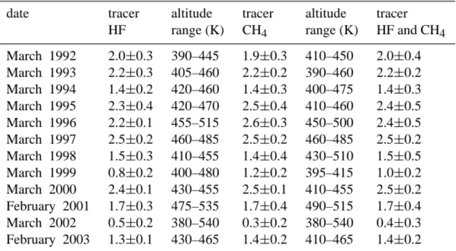
Table 4. Maximum of the local accumulated ozone loss in ppmv in March (February in 2001, 2003) for the winters between 1991–1992 and 2002–2003 in the altitude range (in K), where the loss profile reaches a maximum ±0.1 ppmv, is determined employing both the reference relation using HF and CH4, respectively, as the long-lived tracer for the HALOE measurements inside the entire vortex, with an uncertainty
derived from the uncertainty of the early winter reference function. Additionally, the averages between the maximum derived using HF and CH4 as the long-lived tracer are shown.
date tracer altitude tracer altitude tracer
HF range (K) CH4 range (K) HF and CH4
March 1992 2.0±0.3 390–445 1.9±0.3 410–450 2.0±0.4 March 1993 2.2±0.3 405–460 2.2±0.2 390–460 2.2±0.2 March 1994 1.4±0.2 420–460 1.4±0.3 400–475 1.4±0.3 March 1995 2.3±0.4 420–470 2.5±0.4 410–460 2.4±0.5 March 1996 2.2±0.1 455–515 2.6±0.3 450–500 2.4±0.5 March 1997 2.5±0.2 460–485 2.5±0.2 460–485 2.5±0.2 March 1998 1.5±0.3 410–455 1.4±0.4 430–510 1.5±0.5 March 1999 0.8±0.2 400–480 1.2±0.2 395–415 1.0±0.2 March 2000 2.4±0.1 430–455 2.5±0.1 410–455 2.5±0.2 February 2001 1.7±0.3 475–535 1.7±0.4 490–515 1.7±0.4 March 2002 0.5±0.2 380–540 0.3±0.2 380–540 0.4±0.3 February 2003 1.3±0.1 430–465 1.4±0.2 410–465 1.4±0.2
vortex split and one part rapidly weakened and disinte-grated over eastern Asia. The main vortex centre van-ished more slowly. As in winter 1992–1993, a strong decrease of HCl mixing ratio in the outer part of the vor-tex boundary region was observed by HALOE in Febru-ary. Although the chlorine activation in March was not as strong as in the previous winter 1993–1994, much stronger deviations from the O3-tracer reference
rela-tion in March were observed. During April the HCl lev-els increased towards unperturbed values.
– 1995–1996:
The winter 1995–1996 was the coldest recorded by the US National Meteorology Center (NMC) in 18 years (Manney et al., 1996). From December 1995 the strato-spheric temperatures in the Arctic remained below the PSC threshold until March. The final warming began in early March. Measurements taken by HALOE in the vortex are available for the first part of March and the first part of April. The strongest chlorine activation in March was observed for this twelve-year overview. In April, HCl levels almost completely recovered to un-perturbed values. The deviation from the early winter
reference function O3/HF is the same for March and
April so that no further ozone loss was identified be-tween March and April.
– 1996–1997:
In winter 1996–1997, the polar vortex formed in
November. It was strongly disturbed at the end of
November and reformed again during December. Be-fore the vortex was fully established at the end of
De-cember, horizontal mixing between air from inside and outside the vortex occurred and the minimum tempera-ture remained above the PSC threshold of ≈195 K. Af-ter the reformation, the vortex was very cold and strong. At the 475 K potential temperature level, the lowest temperatures in an 18-year data set were reached in this year in March and April (temperatures were below the PSC threshold until the beginning of April) inside the vortex core (Coy et al., 1997). In March, the vortex core was small and strong whereas the boundary region was wide. PSC occurrence was not possible before Jan-uary therefore no chlorine activation and thus no ozone loss can be expected in November and December 1996. Until the end of March the temperatures in the polar vor-tex were low enough for PSC existence (Fig. 8). Dur-ing mid-February, this potential for chemical ozone loss was enhanced by significant denitrification (Rex et al.,
1999a; Kondo et al., 2000). Deviations from the O3
-tracer early winter reference function are separated into two parts. The chlorine activation is also rather inho-mogeneous with the strongest decrease of HCl inside the vortex core, except for one profile inside the outer vortex measured in the second part of March (Fig. 6, small purple plus sign). The strongest April decrease of HCl mixing ratio was observed in this year because the vortex remained intact and cold for an extremely long period.
– 1997–1998:
The vortex in 1997–1998 was slightly disturbed throughout the whole winter. The final warming be-gan in the middle of March (Pawson and Naujokat,
1999). Minimum temperatures were low enough to acti-vate HCl during December and during January (Fig. 8). Moderate chlorine activation was observed by HALOE in March and only small deviations from the reference
function for O3-tracer occurred. In this winter HALOE
data are only available for March inside the polar vor-tex.
– 1998–1999:
The winter 1998–1998 was unusually warm due to a major stratospheric warming in mid-December (Manney et al., 1999). The vortex in 1998–1999 was very weak and disturbed. Almost no changes in the HCl/HF relation occurred, owing to a small VPSC and
thus very little chlorine activation at the end of February.
However, small deviations from the O3/HF early winter
reference function were found (see discussion below).
– 1999–2000:
In 1999–2000 the Arctic stratosphere was very cold from the middle of November to late March (Manney and Sabutis, 2000). The lowest values of the February HCl mixing ratios for any of the observed years were reached owing to the largest VPSCduring January in the
observed period. HCl mixing ratios are comparable to the low mixing ratios in March 1996. In March 2000, a slight recovery of HCl levels towards unperturbed val-ues became noticeable, with a total recovery at the end of April. The small deviation from the early winter
ref-erence function HF/O3in February strongly increased
in March and continued up to April.
– 2000–2001:
The vortex in 2000–2001 developed during October and November 2000. A strong Canadian warming at the end of November greatly disturbed the vortex. An undis-turbed cold period followed from late December until mid-January. Afterwards, a major warming broke down the vortex in mid-February. During this warming, the vortex drifted over central Europe for a few days and PSC conditions were reached due to a short-term cool-ing of the vortex. The vortex re-established in March and lasted until April. Strong chlorine activation oc-curred in February 2001 (Fig. 6). From March to April HCl levels completely recovered to normal values. In the ozone-tracer relation in February 2001 one profile inside the outer vortex indicates a significant deviation from the early winter reference function. In March and April the early winter reference function is certainly no longer valid, owing to the temporary break-up of the vortex in February, and ozone-tracer profiles scat-ter above the derived function. Therefore, the TRAC technique cannot be applied to ozone-tracer profiles in March and April.
– 2001–2002:
The winter 2001–2002 was a very warm winter. Al-though the temperatures at the end of November reached a record minimum for the period 1979–2001, a strong warming in the second half of December oc-curred so that the vortex significantly weakened. Af-ter the vortex re-established in January, it was weak and warm until it broke down in May. Very little chlorine ac-tivation is noticeable at the end of March 2002 (Fig. 6)
and very little deviation from the O3/HF early winter
reference relation is apparent at the end of April.
– 2002–2003:
In this winter the polar vortex formed in November 2002. It was characterised by very low temperatures in the early vortex and chlorine activation already in
mid-December 2002 (Tilmes et al., 2003a). VPSC was
largest in December for the entire lifetime of the vor-tex. Afterwards, temperatures increased around mid-January and the vortex split twice, once in mid-January and
once in February. Only a small VPSC was derived for
the following month. Some chlorine deactivation was deduced from the HALOE measurements in the vortex in February. In April, HCl had recovered, thus chlo-rine was completely deactivated. The strongest devi-ation from the ozone-tracer reference appeared for the profiles in February, and for one profile in April. A de-tailed analysis of this winter using the TRAC method is described in Tilmes et al. (2003a).
To summarise the temperature conditions for winters be-tween 1991–1992 and 2002-2003, five winters are charac-terised as being cold (1992–1993, 1994–1995, 1995–1996, 1996–1997 and 1999–2000). These winters show a strong
decrease of the HCl mixing ratio in the HCl/HF relation in
spring and strong deviations of O3-tracer profiles from the
early winter reference function. For the cold winters, the
daily VPSC average in 400–550 K between mid-December
and March is between 20×106km3and 40×106km3(shown
below in Sect. 6). Moderate deviations from the O3/HF
ref-erence were found in 1991–1992, 1993–1994, 1997–1998,
2000–2001 and 2002–2003. The daily VPSC average is
be-tween 5×10⁶km3and 15×106km3. In winters 1998–1999
and 2001–2002 there was little chlorine activation and very little deviation from the early winter ozone-tracer reference
function. The value of the daily VPSCaverage does not
ex-ceed 3×10⁶km3for the very warm winters.
The temperature conditions are closely related to the strength of the vortex. A measure of strength of the vor-tex can be derived by summarising those days of each year over the entire winter when the poleward boundary of the vortex (as defined by the Nash et al. (1996) crite-rion) exceeds a certain threshold value of PV. Here 40 PV
units (PVU=10−6K m2/(kg s)) at 475 K is used. For four
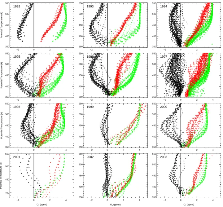
−2 0 2 4 350 400 450 500 550 Potential Temperature (k) 1992 −2 0 2 4 350 400 450 500 550 1993 −2 0 2 4 350 400 450 500 550 1994 −2 0 2 4 350 400 450 500 550 Potential Temperature (k) 1995 −2 0 2 4 350 400 450 500 550 1996 −2 0 2 4 350 400 450 500 550 1997 −2 0 2 4 350 400 450 500 550 Potential Temperature (k) 1998 −2 0 2 4 350 400 450 500 550 1999 −2 0 2 4 350 400 450 500 550 2000 −2 0 2 4 O3 (ppmv) 400 450 500 550 Potential Temperature (k) 2001 −2 0 2 4 O3 (ppmv) 350 400 450 500 550 2002 −2 0 2 4 O3 (ppmv) 350 400 450 500 550 2003
Fig. 9. Vertical profiles (plotted against potential temperature) of O3mixing ratios (red diamonds) measured by HALOE. The ozone mixing
ratios expected in the absence of chemical change ( ˆO3, green diamonds), and the difference between expected and observed O3(1 O3, black diamonds) are shown for the winters between 1991–1992 and 2001-2002 in March (2000–2001, 2002–2003 in February). ˆO3was inferred
using HF as the long-lived tracer and the early winter reference functions (Table 2) from profiles inside the vortex core (squares) and inside the outer vortex (plus signs).
1999–2000, this is the case for more than 100 days of the winter; in 1993–1994, 1996–1997 and 2002–2003, it is 80– 90 days (moderately warm or cold winters), in 1991–1992, 1997–1998, 2000–2001, 2001–2002, 40–63 days (moder-ately warm or warm winter), and 1998–1999 only 20 days of the year (warm winter).
4 Ozone loss profiles and column ozone loss
The chemical ozone loss calculated using the TRAC method should be interpreted as the total amount of ozone destroyed in a period between the time of the early winter reference function and the time of the investigated profile. In this sec-tion, calculated local ozone loss profiles in February/March each year are presented, as well as the monthly average col-umn ozone loss over the course of the entire winter for two different altitude ranges.
−2 0 2 4 350 400 450 500 550 Potential Temperature (k) 1992 −2 0 2 4 350 400 450 500 550 1993 −2 0 2 4 350 400 450 500 550 1994 −2 0 2 4 350 400 450 500 550 Potential Temperature (k) 1995 −2 0 2 4 350 400 450 500 550 1996 −2 0 2 4 350 400 450 500 550 1997 −2 0 2 4 350 400 450 500 550 Potential Temperature (k) 1998 −2 0 2 4 350 400 450 500 550 1999 −2 0 2 4 350 400 450 500 550 2000 −2 0 2 4 O3 (ppmv) 350 400 450 500 550 Potential Temperature (k) 2001 −2 0 2 4 O3 (ppmv) 350 400 450 500 550 2002 −2 0 2 4 O3 (ppmv) 350 400 450 500 550 2003
Fig. 10. As in Fig. 9, but with CH4used as the long-lived tracer and the early winter reference functions (Table 3).
4.1 Vertical ozone loss profiles
For each year, the ozone loss profiles differ with respect to the altitude range where ozone loss occurs, the maximum local ozone loss, the altitude where this maximum loss oc-curs and the extent of homogeneity of the distribution inside the vortex. Vertical ozone loss profiles are calculated using
both HF (Fig. 9) and CH4(Fig. 10) as the chemically
long-lived tracer. These ozone loss profiles (black symbols) are calculated as the difference between the actually measured
ozone concentration O3 (red symbols) and the
correspond-ing ozone proxy ˆO3(green symbols) (e.g. M¨uller et al., 1996;
Tilmes, 2003).
In all winters considered, significant ozone loss mainly arose in the altitude range between 380 and 550 K. At alti-tudes below 380 K the uncertainty of calculated ozone loss profiles increased in most winters because of the increasing influence of mixing processes.
The amount of ozone destroyed at different altitudes and, therefore, the shape of the vertical ozone loss profiles de-pends on the different meteorological conditions inside the polar vortex for each winter. The maximum of the vertical ozone loss profile (in mixing ratio) and the corresponding al-titude range (in potential temperature) is shown in Table 4 for March (or February in the years 2001 and 2003) of each year.