HAL Id: hal-00302162
https://hal.archives-ouvertes.fr/hal-00302162
Submitted on 1 Jan 2003
HAL is a multi-disciplinary open access
archive for the deposit and dissemination of
sci-entific research documents, whether they are
pub-lished or not. The documents may come from
teaching and research institutions in France or
abroad, or from public or private research centers.
L’archive ouverte pluridisciplinaire HAL, est
destinée au dépôt et à la diffusion de documents
scientifiques de niveau recherche, publiés ou non,
émanant des établissements d’enseignement et de
recherche français ou étrangers, des laboratoires
publics ou privés.
Solitary potential structures observed in the
magnetosheath by the Cluster spacecraft
J. S. Pickett, J. D. Menietti, D. A. Gurnett, B. Tsurutani, P. M. Kintner, E.
Klatt, A. Balogh
To cite this version:
J. S. Pickett, J. D. Menietti, D. A. Gurnett, B. Tsurutani, P. M. Kintner, et al.. Solitary potential
structures observed in the magnetosheath by the Cluster spacecraft. Nonlinear Processes in
Geo-physics, European Geosciences Union (EGU), 2003, 10 (1/2), pp.3-11. �hal-00302162�
Nonlinear Processes
in Geophysics
c
European Geosciences Union 2003
Solitary potential structures observed in the magnetosheath
by the Cluster spacecraft
J. S. Pickett1, J. D. Menietti1, D. A. Gurnett1, B. Tsurutani2, P. M. Kintner3, E. Klatt3, and A. Balogh4
1Department of Physics and Astronomy, The University of Iowa, Iowa City, IA, USA 2Jet Propulsion Laboratory, California Institute of Technology, Pasadena, CA, USA 3School of Electrical Engineering, Cornell University, Ithaca, NY, USA
4The Blackett Laboratory, Imperial College, London, UK
Received: 2 January 2002 – Revised: 16 April 2002 – Accepted: 17 April 2002
Abstract. Bipolar pulses of ∼25–100 µs in duration have been observed in the wave electric field data obtained by the Wideband plasma wave instrument on the Cluster spacecraft in the dayside magnetosheath. These pulses are similar in al-most all respects to those observed on several spacecraft over the last few years. They represent solitary potential struc-tures, and in this case, electron phase space holes. When the time series data containing the bipolar pulses on Clus-ter are transformed to the frequency domain by a windowed FFT, the pulses appear as typical broad-band features, ex-tending from the low-frequency cutoff of the bandpass filter,
∼1 kHz, up to as great as 20–40 kHz in some cases, with decreasing intensity as the frequency increases. The upper frequency cutoff of the broad band is an indication of the individual pulse durations (1/f). The solitary potential struc-tures are detected when the local magnetic field is contained primarily in the spin plane, indicating that they propagate along the magnetic field. Their frequency extent and inten-sity seem to increase as the angle between the directions of the magnetic field and the plasma flow decreases from 90◦. Of major significance is the finding that the overall profile of the broad-band features observed simultaneously by two Cluster spacecraft, separated by a distance of over 750 km, are strikingly similar in terms of onset times, frequency ex-tent, intensity, and termination. This implies that the genera-tion region of the solitary potential structures observed in the magnetosheath near the bow shock is very large and may be located at or near the bow shock, or be connected with the bow shock in some way.
1 Introduction
Broad-band electrostatic noise (BEN) was first identified by Scarf et al. (1974) and Gurnett et al. (1976) from measure-ments obtained with a spectrum analyzer in the distant tail. BEN was characterized as bursty and consisting of
broad-Correspondence to: J. S. Pickett ([email protected])
band spectral features usually extending from the lowest fre-quencies measured, up to as high as the plasma frequency, with decreasing intensity as the frequency increases. After this discovery, BEN was observed in several other regions of the Earth with various spacecraft, including the magne-tosheath (e.g. Rodriguez; 1979; Anderson et al., 1982).
In 1994, Matsumoto et al. (1994) made one of the most im-portant new discoveries of the decade with respect to BEN. Upon examining the Geotail PWI time series data, they found that solitary waves of a few milliseconds in duration were re-sponsible for the high frequency part of BEN in the geomag-netic tail as the spacecraft crossed the plasma sheet bound-ary layer. This brought renewed attention to previous obser-vations of solitary waves, also described as solitary bipolar pulses, by S3–3 (Temerin et al., 1982) and Viking (Koskinen et al., 1987), as well as a heightened anticipation of the high time resolution waveform measurements being made on Po-lar and FAST in the mid to late 1990s. Kojima et al. (1999a) have presented some of the characteristics of these solitary waves in the various regions of space. They discuss the sim-ilarities and differences in terms of pulse width, amplitude, flow direction to the magnetic field and flow speed.
By 1998, these pulses were found to be indicative of co-herent potential structures (Franz et al., 1998), with the initial sign of the pulse (positive or negative) determining whether the structure was an electron or ion phase space hole. An in-terferometer on Polar was used to make these measurements. Ergun et al. (1998) found that solitary structures detected by FAST in the auroral acceleration region, called “fast solitary waves”, propagated along the magnetic field at speeds of a few thousands km/s and had amplitudes up to 2.5 V/m.
With the discovery that BEN consists of a series of solitary waves rather than being broad banded, several researchers began performing simulations using experimental data as in-put, in order to explore generation mechanisms. Some of the most important results to come out of these simulations are that electron phase space holes can be generated by several mechanisms. One involves counter-streaming cold electron beams (Goldman et al., 1999) with electrostatic whistlers and
4 J. S. Pickett et al.: Solitary potential structures observed in the magnetosheath lower hybrid waves as an end product. Another involves
dou-ble layers, or strong potential ramps (Singh, 2000; Newman et al., 2001), which accelerate an electron beam and thus, produce electron phase space holes by a spatial two-stream instability. Yet another mechanism involves the nonlinear evolution of the electron beam instability leading to the for-mation of Bernstein-Greene-Kruskal (BGK) potential struc-tures (Omura et al., 1996; Muschietti et al., 1999). Most of these simulations have used the FAST and Geotail data from the auroral acceleration region and geomagnetic tail, respectively, as their input, such that it is unknown at this time whether these simulations are pertinent in other regions of space, such as in the magnetosheath. Kojima et al. (1999a, 1999b) suggest the existence of a common generation mech-anism related to electron dynamics based on a comparison of the time scales of the solitary waves observed in the magne-tosheath to those in the magnetosphere and in the geomag-netic tail with Geotail, FAST and Polar data.
The present study of bipolar pulses makes use of the avail-ability for the first time of identical high time resolution waveform measurements obtained simultaneously on two spacecraft located in the same general region of the dayside magnetosheath near the bow shock. We first describe the waveform receiver and magnetometer that were used to make the Cluster measurements, followed by a presentation of the observations made by the waveform receiver. We continue with an overview of supporting data, particularly the magne-tometer data, that are useful in helping us to understand the wave measurements. We conclude with a discussion of the significance of the observations and a summary of the results.
2 Instrumentation
A Wideband (WBD) plasma wave receiver is mounted on each of the four Cluster spacecraft, which are in an approxi-mately 4 × 20 RE polar orbit around the Earth. The wide-band technique involves transmitting wide-band-limited wave-forms in real time directly to a Deep Space Network ground station using a high-rate data link (Gurnett et al., 1997). WBD processes signals from one of four antennas, measur-ing E-fields via either of two dipole, spherical probe anten-nas located in the spin plane, or B-fields via magnetic search coils located either in the spin plane or along the spin axis. The distance between the two electric field spheres is approx-imately 90 m.
The WBD instrument has three band-pass filter ranges available: 1 kHz to 77 kHz, 50 Hz to 19 kHz, and 50 Hz to 9.5 kHz. In this paper, we will be presenting data ob-tained while the instrument was configured with the 1 kHz to 77 kHz band-pass filter, 8 bits/sample resolution, and the electric Ez(spin plane) antenna selected as the sensor input. In this mode the instrument has a duty cycle of 12.5% and a sample rate of 219.5 kHz. Duty cycling is required because the bit rate exceeds the spacecraft telemetry rate of 220 kbit/s. The WBD gain is automatically updated according to prede-termined criteria in 5 dB steps (a total of 16 possible steps)
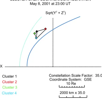
CLUSTER ORBIT LOCATION/CONFIGURATION May 8, 2001 at 23:00 UT
X
Sqrt(Y + Z )2 2
Constellation Scale Factor: 35.0 Coordinate System: GSE Cluster 1
Cluster 2 Cluster 3
Cluster 4 2000 km x 35.0
10 Re
Fig. 1. Locations of the Cluster spacecraft on 8 May 2001 at
23:00 UT and the relative positions of the spacecraft with respect to the nominal bow shock (light blue curve) and magnetopause (dark blue curve). Note that the scale of the spacecraft separations has been expanded 35 times in order to see the details of the separa-tions. Spacecraft 3 (green cross) is the reference spacecraft located at the true position of the Cluster quartet. The data presented in Fig. 2 are from Cluster 1 (black cross) and Cluster 3 (green cross).
over a preselected rate ranging from 0.1 to 27 s in increments of 0.1 s. The update rate for all of the data presented in this paper is 1 s. For further details on the Cluster WBD instru-ment, refer to Gurnett et al. (1997).
The magnetic field investigation (FGM) on Cluster pro-vides accurate, high time-resolution, intercalibrated mea-surements of the magnetic field vector along the Cluster or-bit (Balogh et al., 1997). Each Cluster spacecraft carries an identical instrument consisting of two triaxial fluxgate mag-netometers and an onboard data-processing unit. In order to minimize the magnetic background of the spacecraft, one of the magnetometer sensors is located at the end of a 5.2 m ra-dial boom, and the other is located at 1.5 m inbound from that location. Selection of one of these as the primary sensor is made by ground command. For further information on the Cluster FGM instrument, see Balogh et al. (1997).
3 Experimental observations
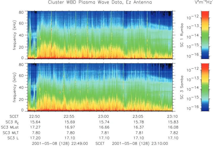
The data presented in this paper were obtained in the day-side magnetosheath at 15.6–15.8 RE. The Cluster spacecraft were outbound and about 1.2–1.4 REearthward of the nom-inal bow shock (see Fig. 1). They were located around +17◦ magnetic latitude and 7.8 Magnetic Local Time. WBD data from spacecraft 1 and 3 were obtained simultaneously during this period and are shown in the spectrograms of Fig. 2. The data were obtained on 8 May 2001 from 22:49 to 23:10 UT.
Fig. 2. Cluster WBD spectrograms from spacecraft 1 and 3 obtained on 8 May 2001 while in the dayside magnetosheath. These spectrograms
show a similar profile of broad-band features (onset, frequency extent, intensity, termination) on both spacecraft, yet the spacecraft are separated by about 750 km.
Data from spacecraft 1 are plotted in the top panel and from spacecraft 3 in the bottom panel (WBD was not telemeter-ing data from spacecraft 2 and 4 at this time). In Fig. 2, frequency is plotted on the vertical axis vs. time on the hori-zontal axis, with colour representing power spectral density. Orbit parameters for spacecraft 3 are provided in columnar format beneath the spectrograms. During this period of time, the electron plasma frequency was 30 kHz or greater and the electron cyclotron frequency was approximately 1 kHz (the basis for the values of these parameters will be briefly dis-cussed in Sect. 4). The interference line seen on both space-craft, but more strongly on spacecraft 3, at about 65 kHz, is associated with the spacecraft batteries. The spectrograms were created on the ground by applying a windowed Fast Fourier Transform (WFT) to the time series.
Most striking in Fig. 2 are the broad-band features ob-served on both spacecraft extending from around 1 kHz up to around 20–40 kHz. The overall profile of these broad-band features (onset, frequency extent, intensity, termination) is exceptionally similar on both spacecraft for this period of time. What makes this observation so unexpected is that the spacecraft are separated by approximately 750 km at this time.
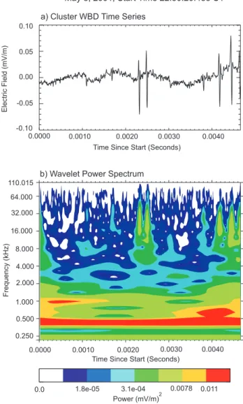
In order to understand the emission that is observed in Fig. 2, it is necessary to look at the waveforms that were used to create the spectrograms. A sample of the calibrated WBD time series from each of the spacecraft is plotted in Figs. 3a (spacecraft 1) and 4a (spacecraft 3). These plots, each cov-ering approximately 4.7 ms, provide the electric field magni-tude, in mV/m, on the vertical axis vs. the elapsed time since the start time shown at the top of the figure, in seconds, on the horizontal axis.
The prominent waveforms seen in Figs. 3a and 4a, e.g. Fig. 4a at 0.0014 s, are what are commonly referred to as bipolar pulses. These are waveform signatures in which a significant, isolated pulse over background is observed, con-sisting of a half sinusoid-like cycle, followed by a similar half cycle having opposite sign. Several of these bipolar pulses are observed in Figs. 3a and 4a on each spacecraft with typ-ical time durations of approximately 70 µs and peak-to-peak fields of 0.1–0.5 mV/m. With respect to the initial direction of the pulses (positive or negative), we see both directions with no clear preference on either spacecraft. Since WBD uses the two spheres from one antenna only in a dipole con-figuration rather than monopole, there is no conclusive way for us to determine whether the solitary potential structures
6 J. S. Pickett et al.: Solitary potential structures observed in the magnetosheath
a) Cluster WBD Time Series
0.0000 0.0010 0.0020 0.0030 0.0040 Time Since Start (Seconds)
-0.10 -0.05 0.00 0.05 0.10 Electric Field (mV/m)
CLUSTER 1 WAVELET ANALYSIS May 8, 2001, Start Time 22:50:20.488 UT
b) Wavelet Power Spectrum
0.0000 0.0010 0.0020 0.0030 0.0040 Time Since Start (Seconds)
0.250 0.500 1.000 2.000 4.000 8.000 16.000 32.000 64.000 110.015 Frequency (kHz) 0.0 1.8e-05 3.1e-04 0.0078 0.011 Power (mV/m)2
Fig. 3. (a) WBD time series data for a 4.7 ms time interval from
Cluster 1 during the time period shown in Fig. 2. Solitary bipolar pulses are observed along with a low-frequency sinusoidal wave-form. The pulses are what creates the broad bands in Fig. 2. (b) Shows the representation of these pulses in frequency and time us-ing a wavelet transform. In this representation, the solitary bipolar pulses are not broad banded.
are positive (implying electron phase space holes) or neg-ative (implying ion phase space holes). However, numer-ous research on this topic, both experimental and theoretical, would suggest that due to the shortness of the pulses, the soli-tary potential structures being observed by the Cluster WBD in the magnetosheath must be electron phase space holes. For example, using the criteria of Kojima et al. (1999a, 199b), we find that a typical duration of a pulse in the magnetosheath, 70 µs, multiplied by the plasma frequency, 30 kHz, gives a characteristic time scale of 2.1 for these solitary waves. This is comparable to the Geotail, Polar and FAST results (values between 1 and 10), implying that these structures are closely
a) Cluster WBD Time Series
0.0000 0.0010 0.0020 0.0030 0.0040 Time Since Start (Seconds)
-0.10 -0.05 0.00 0.05 0.10 0.15 Electric Field (mV/m)
CLUSTER 3 WAVELET ANALYSIS May 8, 2001, Start Time 22:50:19.532 UT
b) Wavelet Power Spectrum
0.0000 0.0010 0.0020 0.0030 0.0040 Time Since Start (Seconds)
0.250 0.500 1.000 2.000 4.000 8.000 16.000 32.000 64.000 110.015 Frequency (kHz) 0.0 2.2e-05 2.9e-04 0.0063 0.012 Power (mV/m)2
Fig. 4. (a) WBD time series data for a 4.7 ms time interval from
Cluster 3 during the time period shown in Fig. 2. Solitary bipolar pulses are observed along with a low-frequency sinusoidal wave-form. The pulses are what creates the broad bands in Fig. 2. (b) Shows the representation of these pulses in frequency and time us-ing a wavelet transform. In this representation, the solitary bipolar pulses are not broad banded.
related to electron dynamics, since the pulse widths are on the order of the electron plasma oscillation periods.
The bipolar pulses with time durations typically ranging from 25 to 100 µs are observed throughout the entire time interval plotted in Fig. 2, with the exception of where the dark blue background (approximately 10−16V2m−2Hz−1) is observed to extend down to frequencies below about 5 kHz, e.g. around 22:49:30, 22:50:10, and 23:03:00 UT. The bipo-lar pulses are represented in the spectrogram as the broad bands which extend from 1 kHz (the lower edge of the fil-ter) up to as great as 20–40 kHz, with power spectral den-sity decreasing as the frequency increases. The WFT used in
Fig. 2 is an inaccurate method for obtaining time-frequency localization, since it imposes a scale or “response interval”
T into the analysis. The inaccuracy arises from the alias-ing of high- and low-frequency components that do not fall within the frequency range of the window (Torrence and Compo, 1998). Thus, the bipolar pulses are more accurately represented in the frequency domain when a wavelet trans-form using a Morlet wavelet is applied to the times series, as shown in Figs. 3b and 4b, since the wavelet transform pro-vides a time-frequency localization that is scale independent. The Morlet wavelet consists of a plane wave modulated by a Gaussian and best approximates the pulses we are trying to analyze. With the wavelet transform we are better able to see what the pulse looks like in time and frequency. We no longer see the broad band, but rather see the peak power as-sociated with the characteristic frequency (time duration, or 1/f) of the pulse as it passes by the spacecraft.
Although the WFT tends to misrepresent the bipolar pulses as broad-band emissions, it does give us valuable insight into the longer term, larger picture of what is going on in this region of space (since the benefits of a wavelet transform would be lost over such a long time interval). For example, as pointed out earlier, the overall frequency-intensity profile is very similar between the two spacecraft. The onset of the bipolar pulses around 22:50:15 UT occurs almost simultane-ously on both spacecraft. Looking at the high-time resolution waveforms, we detect the onset to be approximately 0.9 s ear-lier on spacecraft 3 than on spacecraft 1. If we take this delay time as typical from one spacecraft to another and compare the respective time series from both spacecraft based on this delay, we find that there appears to be no correlation with respect to the individual pulses observed on both spacecraft. Referring to Figs. 3a and 4a, we see that the start time of the time series from spacecraft 3 is about 0.9 s earlier than that of spacecraft 1. While it is tempting for the eye to correlate the first two pulses on both spacecraft, as well as the latter group of four, the amplitudes and time between pulses vary too much from one spacecraft to another for us to conclude that the two spacecraft are viewing the same structures rep-resented by the pulses.
Finally, and most important, is that the frequency extent of the broad bands shown in Fig. 2 give an indication of the du-ration of the individual pulses. For example, the broad bands seen extending up to 40 kHz are indicative of pulses that oc-cur on time scales of 25 µs. Only the WBD instrument on Cluster is capable of resolving these fast pulses in the time domain due to a 1t of 4.5 µs between samples in this mode. Other instruments which detect broad bands in the frequency domain, but which do not provide the waveforms, provide in-conclusive evidence of these bipolar pulses. This is because broad bands similar to those observed in Fig. 2 can also be indicative of electrostatic turbulence when an FFT-type al-gorithm has been used to process the time series. Thus, the waveforms are absolutely essential in determining whether the broad bands represent bipolar pulses or some other sig-nature of the wave electric field.
Some of the other emissions observed in Fig. 2 are
oc-casional bursts of Langmuir waves at the plasma frequency, e.g. at 22:53:42 UT, as well as very weak escaping con-tinuum seen above the broad bands, and a very intense low-frequency emission below about 3 kHz. The contin-uum is obviously not related to the bipolar pulses, since it is propagating above the plasma frequency. Not so clear is the connection, if any, of the low-frequency emission. These low-frequency waves are obvious in the waveforms of Figs. 3a and 4a (the sinusoidal waveforms with a field of about 0.04 mV/m, peak-to-peak), and in the spectra of Figs. 3b and 4b around 500–1500 Hz. Since the filter rolls off steeply below 1000 Hz, we cannot trust the calibration of any emission seen below that frequency. However, the emission observed in Fig. 4b around 1000–1500 Hz can be trusted. We believe that these low-frequency waves are ion acoustic waves based on their falling in the range fπ ≤
f ≤ fpe. They are also quite similar to the low-frequency Doppler-shifted ion acoustic wave packets observed in the solar wind at the L1 point by the WIND spacecraft (Man-geney et al., 1999). We point out that the examples of these low-frequency sinusoidal waves shown in Figs. 3 and 4 are not typical of the intensities of these waves seen through-out Fig. 2. We specifically chose these examples in order to highlight the bipolar pulses.
4 Supporting data
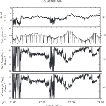
We have examined the DC magnetic field data from the FGM experiment on Cluster for the time period shown in Fig. 2. Panel (a) of Fig. 5 contains the magnitude of the magnetic field for spacecraft 1 (dashed line) and spacecraft 3 (solid line) for a time period that encompasses that of Fig. 2. Panel (b) contains the magnitude of the component of that magnetic field that lies within the spin plane of each space-craft for the same time period. Panels (c) and (d) provide the cone angle for spacecraft 1 and 3, respectively, calculated as the angle between the direction of the magnetic field as measured by FGM and the plasma flow, which we assume is along the X-axis in a GSE coordinate system. No particle data are available from Cluster for this period of time from which to determine the flow direction, since maneuvers had occurred only a few hours before and the particle instruments were put in a saving mode. From Fig. 5, we deduce that the rapid increase in the magnitude of the magnetic field start-ing at about 22:50:15 UT is associated almost entirely with the component of the field that is in the spin plane. Thus, it is clear that WBD detects the bipolar pulses during the time that the local magnetic field lies almost entirely within the spin plane of the spacecraft, which is the plane in which WBD senses. Further, the overall profile of the bipolar pulses, as represented by the broad bands in Fig. 2, very closely approx-imates the profile of the component of the magnetic field con-tained in the spin plane. The magnetic field data also show that spacecraft 3 observes the change to a spin-plane domi-nated direction first, which is consistent with the WBD data. Further, from panels 5(c) and 5(d), it appears as if there is
8 J. S. Pickett et al.: Solitary potential structures observed in the magnetosheath 21:00 22:00 23:00 24:00 21:00 22:00 23:00 24:00 0 20 40 Bspin_plane, nT 1(--) 3( ) U.T. 21:00 22:00 23:00 24:00 0 20 40 60 |B|, nT CLUSTER FGM _ May 8, 2001 1(--) _ 3( ) Cone Angle (Deg.) Cone Angle (Deg.) 30 50 70 90 30 50 70 90 Cluster 1 Cluster 3 (a) (b) (c) (d)
Fig. 5. (a) FGM total magnetic field data from Cluster 1 (dashed
line) and Cluster 3 (solid line). (b) The component of the mag-netic field that lies in the spin plane of the spacecraft for each of Cluster 1 and Cluster 3. (c) and (d) The cone angle, which is the angle between the direction of the magnetic field and the direction of the plasma flow (assumed to be along the GSE X direction), for Cluster 1 and Cluster 3, respectively.
a dependence on the cone angle, i.e. the broad-band features (solitary structures) decrease in intensity and frequency ex-tent (meaning that 1t of the bipolar pulses has increased) or go away, and the low-frequency sinusoidal waves decrease in intensity or go away the closer this angle gets to 90◦.
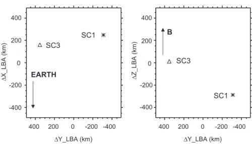
To see whether both spacecraft 1 and 3 lie along the same magnetic field line, we have transformed the position of the spacecraft into a local magnetic field-aligned coordinate sys-tem using the FGM data, as shown in Fig. 6. The 1z axis is parallel to the magnetic field. The 1y axis is in the B × R direction, where R is the radius vector from the Earth to the center of mass of the 4 Cluster spacecraft, and 1x completes the right-handed system. The positions of spacecraft 1 and 3 relative to the center of mass of the four spacecraft in the lo-cal magnetic field-aligned system are shown in Fig. 6. We find that the spacecraft do not lie along the same magnetic field line, but rather lie on different field lines separated by approximately 650 km.
In order to put some of the wave observations into per-spective, we note that the electron cyclotron frequency varies from about 840 to 1120 Hz during the time period of Fig. 2 based on FGM data. The electron plasma frequency is
≥30 kHz based on occasional bursts of Langmuir waves and on the lower frequency cutoff of the continuum that is ob-served during periods of low or absent bipolar pulses. The Kp index is 4 for the three-hour period of 21:00 to 24:00 UT on 8 May 2001. Finally, the solar wind pressure is around 1–
2 nPa, the solar wind speed is close to 500 km/s, the plasma beta is 0.6, and IMF Bzranges from −1 to −6 nT based on ACE data from the L1 point.
5 Discussion
The bipolar pulses that are seen throughout the time inter-val presented in Fig. 2 on 8 May 2001 are consistent with solitary potential structures, in this case electron phase space holes. They are similar in form to the structures observed in the magnetotail and magnetosheath by Geotail, in the auroral acceleration region by FAST, and in the high altitude mag-netosphere, cusp, and near-Earth plasma sheet by Polar, as discussed in the Introduction. Since WBD does not have the capability of configuring itself as an interferometer on any one spacecraft, we are unable to determine the velocity, and thus, the scale size of the structures. Even though the series of solitary pulses observed in Figs. 3 and 4 appear to be cor-related, the time delay between comparable pulses on each spacecraft are not consistent, and the spacecraft do not lie on the same magnetic field line as seen in Fig. 6. Thus, we con-clude that we are not detecting the same bipolar pulses on both spacecraft and we cannot use the two spacecraft as an interferometer to determine velocity and scale size.
With the use of the FGM data, we are able to determine that throughout most of the interval shown in Fig. 2, the mag-netic field is located primarily in the spin plane, as shown in Fig. 5. It is during these times that WBD detects the struc-tures. This is significant because WBD senses only in the spin plane. The structures are, therefore, confined to the plane containing the magnetic field direction.
We have also examined the cone angle, i.e. the angle be-tween the plasma flow direction and the magnetic field, by using FGM data and by assuming that the plasma flow is gen-erally along the −XGSEdirection. For the interval shown in
Fig. 2, we found that this angle is generally between 60 and 90◦. As this angle approaches 90◦, the broad bands associ-ated with the solitary structures decrease in frequency extent and intensity, and the low-frequency waves decrease in inten-sity. Any deviation of the plasma flow from the −X direction is expected to be small, but could result in small changes to the cone angle calculations shown in Fig. 5. It appears that the Cluster WBD data support, to some extent, the findings of Coroniti et al. (1994) that the occurrence of the plasma waves from several hundred Hz to 5 kHz observed by ISEE-3 in the distant magnetosheath are nearly absent when the cone angle is large. However, it is not clear from their data whether the broad-band waves are a combination of bipolar pulses and low-frequency sinusoidal waves, as in the case of Cluster, or just one of these, since waveform data were not available to them.
Based on the detection of the structures only when the magnetic field lies primarily in the spin plane, we conclude that the structures are propagating along the magnetic field. Since changes in the magnetic field in the dayside magne-tosheath are usually related to changes in the IMF, we
be-SC3
SC1
B
EARTH
CLUSTER RELATIVE POSITIONS MAY 8, 2001, 22:50:00 UT SC1 SC3 DZ_LBA (km) DX_LBA (km) DY_LBA (km) 400 200 0 -200 -400 400 200 0 -200 -400 400 200 0 -200 -400 DY_LBA (km) 400 200 0 -200 -400
Fig. 6. Relative positions of Cluster 1
and 3 with respect to the center of mass of the four Cluster satellites in a local magnetic field-aligned coordinate sys-tem, showing that the two spacecraft do not lie along the same magnetic field line, but lie on separate field lines that are separated by about 650 km.
lieve that the IMF is in part controlling the generation of the structures. This is borne out by our observation that the fre-quency extent and amplitude of the structures increases as the angle of the IMF to the plasma flow direction (cone an-gle) decreases significantly from 90◦. This dependence leads to the further conclusion that the bow shock is involved in some way in the generation of the structures, since it reacts to changing IMF and is known to be involved in the generation of electrostatic noise (solitons) that is convected downstream to form a turbulent region at the flanks of the Earth, outside the bow shock (Filbert and Kellogg, 1979).
Onsager et al. (1989) speculated that the broad-band, im-pulsive waves at frequencies greater than about 9 kHz that are polarized parallel to the magnetic field and observed in the magnetosheath downstream from the shock by AMPTE were electron beam mode waves. As in the case of Coroniti et al. (1994), Onsager et al. (1989) did not have the wave-forms available, but their criteria for these waves appear to fit very well the spectral representation of the bipolar pulses observed on Cluster in a similar region. Therefore, we be-lieve that these are one and the same. Onsager et al. (1989) proposed three mechanisms for the generation of the electron beam required in order to produce the waves in the electron beam mode: acceleration by the cross-shock electric field, acceleration by lower hybrid frequency waves, and a mag-netosheath “time of flight” mechanism similar to that in the Earth’s foreshock (Filbert and Kellogg, 1979). In light of the recent findings that the broad-band waves are, in fact, poten-tial structures, these mechanisms will need to be reexamined, but is beyond the scope of the present paper.
With regard to the low-frequency sinusoidal waves around 840–1120 Hz that are believed to be ion acoustic waves, it is possible that these waves are Doppler-shifted up in fre-quency. Since we do not have all of the necessary data at our disposal in order to determine this, we have used
the parameters from a magnetosheath example taken from AMPTE data on 27 December 1984 contained in Onsager et al. (1989). The upstream parameters for this example are very similar to those of ACE for the Cluster data presented here and the spectral features of the broad-band waves ob-served by AMPTE are very similar to those of Cluster. Us-ing the AMPTE parameters gives a maximum Doppler shift of 4 kHz. Since the ion plasma frequency is around 800 to 1000 Hz for the data shown in Fig. 2, we would expect Doppler-shifted ion acoustic waves no higher than 4 kHz. This is consistent with the low-frequency sinusoidal waves observed in Fig. 2, which are observed up to about 3 kHz. The solitary potential structures (bipolar pulses) are unlikely to be affected by a Doppler shift, because they are believed to be propagating at velocities on the order of a few thou-sand km/s, which is considerably higher than the magne-tosheath velocity of 200–400 km/s. The low-frequency sinu-soidal waves that are detected at the same time as the bipo-lar pulses may be important in understanding how the pulses are generated. One thing that is clear is that the detection of this lower frequency sinusoidal wave in the spin plane, which also contains the major component of the magnetic field, im-plies that this wave has a very measurable electric field com-ponent along the magnetic field and could thus, potentially provide a trapping mechanism for electrons.
The major conclusion to be derived from the Cluster WBD data obtained by two spacecraft in the dayside mag-netosheath on 8 May 2001 is that the generation region must be extremely large. The fact that onsets of the bipolar pulses are observed almost at the same time on two spacecraft lo-cated about 750 km apart, and that the duration of the pulses and intensities of the pulses are similar and change similarly over time points most strongly to this conclusion. Whether the solitary potential structures that are observed in the mag-netosheath are generated in the bow shock and propagate
10 J. S. Pickett et al.: Solitary potential structures observed in the magnetosheath to each individual spacecraft along different magnetic field
lines, or whether they are generated locally at each space-craft in response to processes occurring at the bow shock is not currently known. We note, however, that although the separation of the two spacecraft is 750 km, spacecraft 3 is only 153 km closer to the bow shock than spacecraft 1. This would mean that if the structures were generated at the bow shock, they would only be travelling at 170 km/s based on the delay of 0.9 s from spacecraft 3 to 1, which is inconsis-tent with all other measurements of the velocities of this type of structure. Thus, it might be reasonable to assume that the structures are generated locally at each spacecraft in response to processes occurring at the bow shock, with the messen-gers of those processes travelling to each spacecraft at about 200 km/s.
6 Summary
The Cluster WBD instrument has obtained digital wave-form measurements of the wave electric field sampled at 219.5 kHz in the dayside magnetosheath from two space-craft separated by about 750 km. The waveforms show the presence of solitary bipolar pulses with time durations on the order of 25–100 µs. These bipolar pulses are consistent with solitary waves observed in the magnetosheath and from other regions of space in which they are interpreted as soli-tary potential structures, and in this case, more specifically as electron phase space holes. There is no correlation between the individual structures from one spacecraft to another at these large distances. A spectrogram of these data covering a 21-minute time interval primarily shows broad-band features covering the range of 1 kHz (the lower limit of the bandpass) up to 40 kHz, which is the typical representation of a pulse when using a windowed Fourier Transform.
The profiles of these broad-band features (onset, frequency extent, intensity, termination) when viewed over the 21-min interval are strikingly similar on the two Cluster spacecraft. This profile is also similar to that of the amplitude of the component of the magnetic field that lies in the spin plane of the spacecraft, the only plane that is sampled by WBD. This implies that the solitary potential structures associated with these broad-band features are propagating along the mag-netic field, since they are not observed when the magmag-netic field lies primarily along the spin axis. The intensity and frequency extent of the broad-band features also appear to be dependent on the angle between the direction of the magnetic field and the direction of the plasma flow, with the intensity and frequency extent increasing as the angle decreases from 90◦. Finally, and most important, the good correlation be-tween the overall profile of the structures on one spacecraft and that on the other, when separated by 750 km, implies that the generation region, whether local, at, or near the bow shock, is large.
Cluster WBD should be in a better position to observe these solitary potential structures in the magnetosheath, as well as in all other regions of its orbit, during the time period
of 1 February through 30 May 2002. During this period, the interspacecraft separation distances will be on the order of 100–300 km. We hope to be able to positively identify iden-tical structures on more than one spacecraft, so that we can determine velocity and scale size. In addition, this will give us an opportunity to examine the all important issue of how the structures propagate, grow and decay. We also hope to be able to determine whether the structures coalesce early in their generation. With the aid of the potential control experi-ment, ASPOC, to shield photoelectrons from the spacecraft, we hope to be able to measure electrons to lower energies on the dayside than is possible without potential control. Elec-tron and ion data, together with the WBD and other wave data, and electric and magnetic field data from multi-Cluster spacecraft, should provide us with the first opportunity to de-termine experimentally the generation mechanism, propaga-tion, growth, and decay properties of these structures.
Acknowledgements. We acknowledge the support of NASA
God-dard Space Flight Center through Contract NAS5–30730 and Grant NAG5–9947. Portions of the work were performed at the Jet Propulsion Laboratory, California Inst. of Tech. under contract with NASA. We acknowledge the ACE spacecraft investigation team for the use of their browse magnetic field and ion data. We thank the following individuals who were crucial in obtaining and processing the data: R. Huff, J. Dowell, R. Brechwald and I. Christopher of the University of Iowa, C. Abramo and A. Horton at DSN, K. Yearby and I. Willis of Sheffield University and M. Hapgood of Ruther-ford Appleton Laboratory. We also acknowledge use of some very valuable analysis tools supplied by GSFC, namely, SSCWeb and CDAWeb.
References
Anderson, R. R., Harvey, C. C., Hoppe, M. M., Tsurutani, B. T., Eastman, T. E., et al.: Plasma waves near the magnetopause, J. Geophys. Res., 87, 2087–2107, 1982.
Balogh, A., Dunlop, M. W., Cowley, S. W. H., Southwood, D. J., Thomlinson, J. G., et al.: The Cluster Magnetic Field Investig-taion, Space Sci. Rev., 79, 65–92, 1997.
Coroniti, F. V., Greenstadt, E. W., Moses, S. L., Tsurutani, B. T., and Smith, E. J.: On the Absence of Plasma Wave Emissions and the Magnetic Field Orientation in the Distant Magnetosheath, Geo-phys. Res. Lett., 21, 2761–2764, 1994.
Ergun, R. E., Carlson, C. W., McFadden, J. P., Mozer, F. S., De-lory, G. T., et al.: FAST satellite observations of large amplitude solitary structures, Geophys. Res. Lett., 25, 2041–2044, 1998. Filbert, P. C. and Kellogg, P. J.: Electrostatic Noise at the Plasma
Frequency beyond the Earth’s Bow Shock, J. Geophys. Res. 84, 1369–1381, 1979.
Franz, J. A., Kintner, P. M., and Pickett, J. S.: POLAR observa-tions of coherent electric field structures, Geophys. Res. Lett., 25, 1277–1280, 1998.
Goldman, M. V., Oppenheim, M. M., and Newman, D. L. Nonlin-ear two-stream instabilities as an explanation for auroral bipolar wave structures, Geophys. Res. Lett., 13, 1821–1824, 1999. Gurnett, D. A., Frank, L. A., and Lepping, R. P.: Plasma waves in
the distant magnetotail, J. Geophys. Res., 81, 6059–6071, 1976. Gurnett, D. A., Huff, R. L., and Kirchner, D. L.: The Wide-Band Plasma Wave Investigation, Space Sci. Rev., 79, 195–208, 1997.
Kojima, H., Matsumoto, H., and Omura, Y.: Electrostatic solitary waves observed in the geomagnetic tail and other regions, Adv. Space Res., 23, 1689–1697, 1999a.
Kojima, H., Omura, Y., Matsumoto, H., Miyagut, K., and Mukai, T.: Characteristics of electrostatic solitary waves observed in the plasma sheet boundary: statistical analyses, Non. Proc. Geo-phys., 6, 179–186, 1999b.
Koskinen, H. E. J., Bostrom, R., and Holback, B.: Viking observa-tions of solitary waves and weak double layers on auroral field lines, Phys. of Space Plasmas, SPI conference proceedings and reprints series, 7, 147–156, 1987.
Mangeney, A., Salem, C., Lacombe, C., Bougeret, J.-L., Perche, C., et al.: WIND observations of coherent electrostatic waves in the solar wind, Ann. Geophysicae, 17, 307–320, 1999.
Matsumoto, H., Kojima, H., Miyatake, T., Omura, Y., Okada, M., et al.: Electrostatic solitary waves (ESW) in the magnetotail: BEN wave forms observed by GEOTAIL, Geophys. Res. Lett., 21, 2915–1918, 1994.
Muschietti, L., Ergun, R. E., Roth, I., and Carlson, C. W.: Phase-space electron holes along magnetic field lines, Geophys. Res. Lett., 26, 1093–1096, 1999.
Newman, D. L., Goldman, M. V., Ergun, R. E., and Mangeney, A.:
Formation of double layers and electron holes in a current-driven space plasma, Phys. Rev. Lett., 87, 255 001-1–255 001-4, 2001. Omura, Y., Kojima, H., Miki, N., and Matsumoto, H.:
Two-dimensional electrostatic solitary waves observed by Geotail in the magnetotail, Adv. Space Res., 24, 55–58, 1999.
Onsager, T. G., Holzworth, R. H., Koons, H. C., Bauer, O. H., Gur-nett, D. A., Anderson, R. R., Luhr, H., and Carlson, C. W.: High-Frequency Electrostatic Waves Near Earth’s Bow Shock, J. Geo-phys. Res., 94, 13 397–13 408, 1989.
Rodriguez, P.: Magnetosheath Electrostatic Turbulence, J. Geo-phys. Res., 84, 917–930, 1979.
Scarf, F. L., Frank, L. A., Ackerson, K. L., and Lepping, R. P.: Plasma wave turbulence at distance crossings of the plasma sheet boundaries and the neutral sheet, Geophys. Res. Lett., 1, 189– 192, 1974.
Singh, N.: Electron holes as a common feature of double-layer-drive plasma waves, Geophys. Res. Lett., 27, 927–930, 2000. Temerin, M., Cerny, K., Lotko, W., and Mozer, F. S.: Observations
of double layers and solitary waves in the auroral plasma, Phys. Rev. Lett., 48, 1175–1179, 1982.
Torrence, C. and Compo, G. P.: A practical guide to wavelet analy-sis, Bull. Amer. Meteor. Soc., 79, 61–79, 1998.