HAL Id: hal-03006568
https://hal.archives-ouvertes.fr/hal-03006568
Submitted on 19 Apr 2021HAL is a multi-disciplinary open access archive for the deposit and dissemination of sci-entific research documents, whether they are pub-lished or not. The documents may come from teaching and research institutions in France or abroad, or from public or private research centers.
L’archive ouverte pluridisciplinaire HAL, est destinée au dépôt et à la diffusion de documents scientifiques de niveau recherche, publiés ou non, émanant des établissements d’enseignement et de recherche français ou étrangers, des laboratoires publics ou privés.
Distributed under a Creative Commons Attribution| 4.0 International License
2A and EO1 data in Kneiss Archipelago Gulf of Gabes,
Tunisia
R. Katlane, Cécile Dupouy, B. El Kilani, J.-C. Berges
To cite this version:
R. Katlane, Cécile Dupouy, B. El Kilani, J.-C. Berges. Estimation of chlorophyll and turbidity using sentinel 2A and EO1 data in Kneiss Archipelago Gulf of Gabes, Tunisia. International Journal of Geosciences, Scientific Research 2020, 11, p. 708-728. �10.4236/ijg.2020.1110035�. �hal-03006568�
https://www.scirp.org/journal/ijg ISSN Online: 2156-8367
ISSN Print: 2156-8359
DOI: 10.4236/ijg.2020.1110035 Oct. 30, 2020 708 International Journal of Geosciences
Estimation of Chlorophyll and Turbidity Using
Sentinel 2A and EO1 Data in Kneiss Archipelago
Gulf of Gabes, Tunisia
Rim Katlane1, Cécile Dupouy2, Boubaker El Kilani3, Jean Claude Berges4
1GEOMAG (LR19ES07)/PRODIG (UMR 8586), University of Mannouba-Tunis Campus Universities Manouba, Tunisia 2IRD, Aix-Marseille U., U. Toulon, CNRS, M.I.O., France
3GEOMAG (LR19ES07), University of Mannouba, Tunis, Tunisia 4PRODIG, Sorbonne University Paris-Cité, Paris, France
Abstract
Multispectral and hyperspectral sensor data of the bio-optical parameters with a high spatial resolution are important for monitoring and mapping of the coastal ecosystems and estuarine areas, such as the Kneiss Islands in the Gulf of Gabes. Sentinel 2 S2A and Hyperion Earth observing-1 (EO1) imag-ing sensors reflectance data have been used for water quality determination and mapping of turbidity TU and chlorophyll Chl-a in shallow waters. First, we applied a tidal swing area mask based on uncorrelated pixel via 2D scatter plot between 665 nm and 865 nm to eliminate the overestimation of the con-centration of water quality parameters due to the effect of the bottom reflec-tion. The processing for mapping and validating Chl-a, Turbidity S2A, and EO1 were performed using a relation between reflectance bands and in situ measurements. Therefore, we were able to validate the performance of the case 2 regional coast colour processor (C2RCC) as well as our region-adapted empirical optical remote sensing algorithms. Turbidity was mapped based on the reflectance of 550 nm band for EO1 (R2 = 0.63) and 665 nm band for S2A
(R2 = 0.70). Chlorophyll was mapped based on (457/528 nm) reflectance ratio
(R2 = 0.57) for EO1 and (705/665 nm) reflectance ratio (R2 = 0.72) for the S2A.
Keywords
Hyperspectral, Kneiss Islands, Multispectral, Shallow Waters, Water Quality
1. Introduction
Satellite data are effectively used in the physical characterization of some
com-How to cite this paper: Katlane, R., Du-pouy, C., El Kilani, B. and Berges, J.C. (2020) Estimation of Chlorophyll and Tur-bidity Using Sentinel 2A and EO1 Data in Kneiss Archipelago Gulf of Gabes, Tunisia.
International Journal of Geosciences, 11, 708-728.
https://doi.org/10.4236/ijg.2020.1110035
Received: September 14, 2020 Accepted: October 27, 2020 Published: October 30, 2020 Copyright © 2020 by author(s) and Scientific Research Publishing Inc. This work is licensed under the Creative Commons Attribution International License (CC BY 4.0).
http://creativecommons.org/licenses/by/4.0/
DOI: 10.4236/ijg.2020.1110035 709 International Journal of Geosciences
plex ecosystems, such as the estuarine system of the Kneiss Islands in the Gulf of Gabes.
Multispectral and hyperspectral remote sensing of the bio-optical parameters can be important data for mapping, classification, and monitoring of the coastal ecosystems and estuarine areas [1]. Hyperspectral imaging and empirical rela-tionships between reflectances obtained by optical remote sensing algorithms have been used to assess water quality [2][3][4][5][6], allowing chlorophyll a (Chl-a) and turbidity TU mapping in shallow waters.
Several authors have analysed surface water by applying algorithms or em-pirical relationships between water constituent and reflectance [1][7][8] using ocean color sensors like SeaWiFS, MERIS, and MODIS. The semi-analytical, empirical bio-optical models, band ratio or chlorophyll quantification algo-rithms have been developed mainly according to the concentration range of in situ Chl-a and turbidity (case I or case II water) and also in terms of the specific wavelengths available in the multi or hyperspectral sensors (MODIS, SeaWiFS, EO1, MERIS, SENTINEL, etc.) [9]-[17]. The high spatial resolution and the ex-cellent Chl-a spectral quality bands of the Sentinel 2A (S2A) data provide clear and precise information on the optical properties of water. Various turbidity mapping algorithms have been developed for different regions using multi or hyperspectral satellite data. The assessment of suspended matter relies on field spectrometry data merged with the satellite data and is obtained from a combi-nation of channels at several wavelengths [18] or a single wavelength algorithm [19]. These applications are suitable for the coastal or estuarine areas at a coarse spatial resolution (250 m - 1000 m). Besides, Landsat or SPOT data have been used to retrieve case II water’s optical properties [16][20].
Inland, coastal and estuarian shallow water area is dependent on the dynamics of sediments originated by wave erosion, tidal currents, hydrological parameters, biological and chemical constituent of water. For that this region presents a complex optical proprieties of case 2 waters, they are influenced by turbidity TU, Total suspended sediments TSS, dissolved matter, organic matter, microorgan-ism, inorganic particulates matter from minerals [21].
Monitoring of water quality from remote sensing data depends on the spectral characteristic of water. So, to have the real optical properties of the water in shallow water, it is important to apply the atmospheric correction and to remove the effects of the bottom reflection.
Several atmospheric correction algorithms have been created and used for case 2 waters. ACOLITE developed to Landsat 8 OLI and S2A (MSI) in two steps: 1) A Rayleigh correction for scattering by air molecules, using a LookUp Table generated using 6SV. 2) An aerosol correction based on the assumption of black SWIR bands over water caused by the extremely high pure-water absorption, and an exponential spectrum for multiple scattering aerosol reflectance [22].
Case 2 Regional Coast Colour processor C2RCC is developed for optically complex Case 2 waters, which use a large database of simulated water leaving
ra-DOI: 10.4236/ijg.2020.1110035 710 International Journal of Geosciences
diance and TOA radiances. It is based on neural network technology and has been trained in extreme ranges of scattering and absorption properties [23].
Sen2cor available in the Sentinel 2 toolbox more adapted to extract L2 prod-ucts and classify image often used continental area [24], but also to give good results in inland and coastal waters [25].
Polynomial based algorithm applied to MERIS POLYMER was developed for MERIS data to remove the influence of sun glint and retrieve ocean color pa-rameters and spectrum of water leaving radiance, [26]. As regards the effect of reflection of the seabed, more correction has been applied [27][28] and this is to extract the reflectance of the water column and avoid the overestimation of the concentrations of the water quality parameters, especially the turbidity [29].
The objectives of this study are to assess the performances of both hyperspec-tral Hyperion data EO1 and Sentinel 2A data to retrieve Chl-a and TU validated by in situ observations of these two parameters in estuarine Kneiss archipelago.
2. Materials and Methods
2.1. Study Area
The Kneiss Islands lie in Skhira bay in the Gulf of Gabes in the southeastern coast of Tunisia at Khaouala village. This archipelago is located about 3.5 Km off the continent with an area of about 5850 ha. Figure 1 shows the geographic lo-cation of the study area with the digital seabed model established from the dig-itization of the bathymetric data. The entire archipelago is a part of the shallow water that has emerged above the waterline. It belongs to a shallow extended platform cut into by tidal channels that become visible at low tide like Oued Ed-dam [30][31]. The Kneiss archipelago is made up of four islets: Dziret el Bassila, Dziret El Hjar, Dziret El Laboua, and Dziret El Gharbia. The highest point is only 7 m above the sea-level, and the altitude is usually less than 2 m. The hy-drodynamics of this area are influenced by semi-diurnal tides with a maximum amplitude of 2 m [31]. The flow direction is south-west with a speed of 0.1 ms−1
and the main direction of the ebb is northeast with a speed of 0.08 ms−1[32][33]
[34]. This area is characterized by the presence of submerged tidal channels. Coastal currents have a principal direction of NNE-SSO with a speed of 2 ms−1.
The swelling is reduced by shallow water and bottom vegetation [35]. All the is-lets have a backbone of calcareous sandstone, and Bassila is occupied by sebkhas chotts, especially maritime marshland [36]. The collective name of Kneiss Is-lands (plural of Knissa, meaning church in Arabic) originates from the presence of a Christian religious building whose foundation dates back to late antiquity. Indeed, the geo-archaeological studies [37] locate the monastery of Saint Ful-gence of Ruspe at the beginning of the VIth century on the island of El Laboua, which is central to this group of islets. The small islets continued to be united until the historical period [33][38]. The Kneiss archipelago is the outlet part of a huge watershed (Leben). The vast indentation bordered by large Salicornia swamps corresponds to an old estuary [30]. It is an alluvial cone of a paleo Oued
DOI: 10.4236/ijg.2020.1110035 711 International Journal of Geosciences Figure 1. Geographic location, morphology under sea and photographs with their position in the map.
that threw itself into the sea and is remodeled by the littoral drift (according to the configuration of the coast and the direction of the prevailing winds). Sedi-ments accumulate in this area due to the existence of the high depths of the Gulf of Gabes [30] [31] [39]. The archipelago region of Kneiss has been listed as RAMSAR site in 2007, Important Bird Area (IBA) in 2003, and Specially Pro-tected Area of Mediterranean Importance (SPAMI) in 2001.
2.2. Satellite Data
The Sentinel 2 is a wide-swath, high-resolution, multi-spectral imaging mission. Sentinel 2 multispectral imagery (MSI) data, characterized by a high spatial resolution (20 m, 10 m), 13 spectral bands, and a 12 bits radiometric resolution, appear as an appropriate tool to map and retrieve information in shallow water regions [40][41][42]. Its optical instrument samples in 13 spectral bands: four bands at 10 m spatial resolution (490 nm (B2), 560 nm (B3), 665 nm (B4), 842 nm (B8)), six bands at 20 m spatial resolution (705 nm (B5), 740 nm (B6), 783 nm (B7), 865 nm (B8a), 1610 nm (B11), 2190 nm (B12)) and three bands at 60 m spatial resolution (443 nm (B1), 945 nm (B9) and 1375 nm (B10). The Level-2A product provides Bottom of Atmosphere (BOA) reflectance images derived from
DOI: 10.4236/ijg.2020.1110035 712 International Journal of Geosciences
the associated Level-1C products. Therefore, each Level-2A product is also composed of 100 km2 tiles in cartographic geometry (UTM/WGS84 projection).
The Earth Observing 1 (EO1) satellite has three imaging sensors: the multis-pectral Advanced Land imager (ALI), the hypersmultis-pectral Hyperion sensor, and the Atmospheric Corrector (AC). ALI is a new, more compact, and slightly en-hanced version of the legacy TM. The short-lived AC was a moderate resolution hyperspectral sensor. Hyperion is a hyperspectral imager capable of resolving 220 spectral bands (from 0.4 to 2.5 micron) with a 30 m ground resolution. The instrument images a 7.5 km by 100 km surface area. Since the launch of EO1 in late 2000, Hyperion is the only source of space-borne hyperspectral imaging data at a fine resolution and is used for mapping water quality in estuarine and coastal regions [43].
2.2.1. Hyperion Data
EO1/Hyperion satellite imagery of January 22, 2009 (only image available for the study area) was downloaded from NASA Website (https://earthexplorer.usgs.gov). Among the 242 bands of EO1, only 39 bands (457 µm b11 to 874 µm b52) were retained. All other bands were dropped because they either do not contain a data record or they are of poor spectral quality due to the presence of streaks. Figure 2 shows all the radiance values along a transect. It can be noticed that, while more than half of Hyperion spectral bands provide vital information on the ground, only a limited set of these bands is usable for the sea. This feature is re-lated to the high absorption in the near-infrared domain. The Hyperion sensor lacks accuracy, and the signal-to-noise ratio is high.
2.2.2. Sentinel 2A Data
In this study, we processed and analyzed a Sentinel 2A (S2 MSI level 1C) image acquired on May 21, 2017. The data were downloaded from the Sentinel Scien-tific Data Hub (https://scihub.copernicus.eu/). Sentinel application platform
Figure 2. Hyperion radial transect taken from an image of 22 January. The transect path is marked by a white line on the composite color image (up). The corresponding radiance values (W/m2∙str∙µm−1) are displayed for all Hyperion channels (bottom).
DOI: 10.4236/ijg.2020.1110035 713 International Journal of Geosciences
(SNAP) version 6.0 on Windows (64 bits) was downloaded
(https://step.esa.int/main/download/snap-download/). It is a typical architecture for all Sentinel Toolboxes and is being jointly developed by Brockmann Consult, Array Systems Computing, and C-S.
2.2.3. In-Situ Datasets
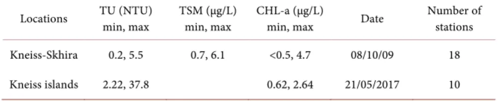
Estuarine Kneiss Islands areas falling under sub-arid climate are challenging en-vironments for remote sensing assessments due to various land Sebkhas, soil, tidal area, shallow waters, seagrasses, slikke, schore to name a few. Water sam-ples were collected on October 8, 2009, May 21, 2017 between 10 a.m. and 12 p.m. from the sites; turbidity TU (NTU), chlorophyll Chl-a (µg/L), and total suspended matter (TSM) (µg/L). A summary is given in Table 1. For each sta-tion, a 10-L water sample was collected and transported to the laboratory for measurement. Turbidity was obtained with a nephelometric method, and the Chl a was measured by the spectrophotometric method. All measurements were realized in the GREEN LAB laboratory (Tunisia). Full details of the method can be found in REVAMP protocols [44].
2.3. Methodology
Preprocessing, processing, and validation of the in-situ data were carried out on the EO1 and S2A data. Figure 3 shows a detailed flowchart of the adopted methodology. Pretreatment was carried out to correct the effects of the atmos-phere. In fact, the spectral resolution of Hyperion bands makes it necessary to eliminate the disturbances caused by atmospheric effects (i.e., water vapor, aerosols). The corrections were based on the 6s software [45] [46] which has a radiative transfer model in the visible and near-infrared spectrum with a resolu-tion of 5 nm. In order to speed up the calcularesolu-tions, the second-order spherical albedo term was discarded. Thus, the atmospheric correction was reduced to a linear transformation based on absorption and a backscatter term. These coeffi-cients were considered as constants on a few square kilometre’s scenes.
The corrections depend on three atmospheric parameters: the ozone content, the water vapor, and the optical thickness at 550 nm. Only the first parameter was extracted from the climatology provided by 6s. The water vapor content was provided by the NOAA/NCEP-DOE (https://psl.noaa.gov/) reanalysis. The op-tical thickness was inferred from the Hyperion measurements at the sea of Gabes and by reversal of the 6s model. The 6SV 2.1 version was downloaded from
http://6s.ltdri.org site.
Table 1. Summary of in-situ measurement.
Locations TU (NTU) min, max TSM (µg/L) min, max CHL-a (µg/L) min, max Date Number of stations Kneiss-Skhira 0.2, 5.5 0.7, 6.1 <0.5, 4.7 08/10/09 18 Kneiss islands 2.22, 37.8 0.62, 2.64 21/05/2017 10
DOI: 10.4236/ijg.2020.1110035 714 International Journal of Geosciences
Data Processing of EO1 and S2A Images
Based on the concept that the wavelengths are the vehicles of the information we have try to visualize all the bands and eliminates the one which presents a bad radiometric recording especially for the EO1 data or we have to keep 39 bands of the 242 available. In the second step, we applied the pretreatments and the masks; continent and shallow water to minimize the effect of the bottom reflec-tion in certain areas. Finally, the adopted approach to TU and CHL-a product validation is by “match-up” validation, comparing the data value for all wave-lengths pixel with an in situ measurement from a location within that pixel and acquired almost simultaneously. In order to make all scatter plot possible and extract a better regression between them, processing and interpretation ap-proach are illustrated in Figure 3.
3. Results
3.1. Hyperion EO1 Data
A false RGB (711 nm, 620 nm, and 528 nm) Color composition and continental mask of the Hyperion data cube is shown in Figure 4.
Four samples of different water color and depth were chosen on the image for extracting the spectral profile. Samples were taken and materialized by decreas-ing order of depth. Sampldecreas-ing 1 was located in the deepest part of the study area at tidal channels (depth of 50 cm), and sample 4 was located in shallow water (depth of 30 cm). The spectral responses of these different depths clearly show that a shallow waters mask coinciding with areas of swaying tide must be applied at the time of the satellite overpass.
DOI: 10.4236/ijg.2020.1110035 715 International Journal of Geosciences Figure 4. (a) RGB EO1 (b40:711 nm/b30:620 nm/b20:528 nm) with sampling points positions on the Hyperion image in yellow, and (b) reflectance spectra of the four sampling points.
3.1.1. Estimation of Chl-a Using Hyperion EO1 Data
In order to estimate Chl-a from EO1, we adopted the ratio between blue to green bands. This ratio is based on the in situ measurements that were made in the Gulf of Gabes [8][47][48][49] and Kneiss Islands (Table 1) and from the spec-tral signatures extracted via the satellite EO1. Figure 5 shows the best scatter plot between the generating blue to green ratio and the measured Chl-a contents (R2 = 0.578). The resulting distribution of Chl-a as calculated from this
regres-sion model using EO1 reflectance (Figure 5(b)) is different from the distribu-tion of the water color as shown in the RGB composidistribu-tion except for the shallow water region (less than 50 cm of depth) which are red-flagged in the map.
Therefore, we accepted the blue to green ratio to extract Chl-a concentration. Rrs is the remote sensing reflectance defined by:
0 0 Rrs Lw Ed + + = where 0 w L+ and Ed0
+ are respectively the water-leaving radiance and the
down-ward irradiance just above the sea surface. The equation is given as: Rrs457 Rr Chl-a 0. s528 005 = (1)
DOI: 10.4236/ijg.2020.1110035 716 International Journal of Geosciences Figure 5. (a) Spatial distribution of the Chl-a EO1 (b11:457 nm/b18:528 nm), (b) Correlation between the ratio (457 nm/528 nm) was calculated from the EO1 data and chlorophyll a measured from water samples.
3.1.2. Estimation of TU Using Hyperion EO1 Data
The turbidity estimation algorithms via satellite data have often been carried out according to the types of coastal or oceanic water and to the range of turbidity [50] [51] [52]. The best linear regression is R2 = 0.6382 (Figure 6) was
estab-lished between the reflectance at 550 nm wavelength of the available EO1 bands and the in situ turbidity data. The spatial distribution of the TU (Figure 6) data, deduced via the 550 nm wavelength, maps the sediment transport via the tidal channels and the direction of the currents in the study area. A slight overestima-tion of NTU concentraoverestima-tion in the shallow water region (less than 50 cm of water depth, visible on Figure 6(a) in red) can be noticed. Thereby an empirical rela-tion to map turbidity in the Kneiss Islands via EO1 data is given as:
(
)
TU=0.218 Rrs550 +11.248 (2)
3.2. Sentinel 2 Data
For a detailed mapping of Kneiss Archipelago, we used S2A sentinel data at 10 m and 20 m spatial resolution. These data were registered on the same day as that of the in situ samplings (May 21, 2017). The preprocessing was carried out by the SNAP software. We’ve tested The L2 C2RCC SNAP toolbox product, par-ticularly, Rhow 400 - 1200 nm; (atmospherically corrected angular dependent water leaving reflectance Rhow = Rrsπ diffuse attenuation coefficients m−1),
conc_tsm (total suspended matter dry concentration gm−3) and conc_chl
DOI: 10.4236/ijg.2020.1110035 717 International Journal of Geosciences Figure 6. (a) Spatial distribution of the TU EO1 with continental mask, (b) correlation between the Rrs 550 nm and TU (NTU) measured from water samples.
In addition, we have the possibility to add additional background information such as salinity, elevation, ozone, temperature, and air pressure [53]. Figure 7(a) proves the locations of the measuring stations. The quality of Sentinel spatial and radiometric data was clearly visible as it showed the morphology of the es-tuarine areas of the Kneiss Islands. The remote sensing reflectance Rrs derived from S2A using C2RCC for the in situ measurement positions are displayed in Figure 7(b).
3.2.1. Shallow and Tidal Area Mask
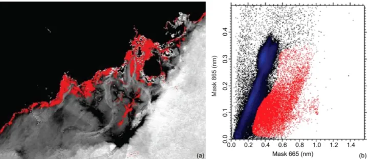
Kneiss islands are a tidal area and several regions have very shallow water for that we apply a relationship between 665 nm and 865 nm that is limited to tur-bidity with reflectance increasing in TU up to ~20 NTU for Rrs (645) and up to ~1000 NTU for Rrs (859) [19]. To better understand the relationship between these two wavelengths for our area, we established a 2D scatter plot between 665 nm and 865 nm (Figure 8(b)). These two wavelengths were highly correlated except for certain pixels. To delineate the area with high turbidity and to extract all uncorrelated pixel water (Figure 8(a)), identification was carried out to locate those pixels. Their positions coincided with the shallow water region, which was a tidal swing area (deepness less than 50 cm). The same regions showed an over-estimation for the concentration of Turbidity due to the effect of bottom reflec-tion. Therefore, we have created a mask based on these non-correlated pixels in order to eliminate the areas influenced by the reflection of the seabed (Figure 8).
DOI: 10.4236/ijg.2020.1110035 718 International Journal of Geosciences
3.2.2. Estimation of Chl-a Using Sentinel 2A Data
A visualization of all the bands and S2A C2RCC product was carried out, also we tried to test and seek the best linear relationships and regressions between the wavelengths and the in situ measurements of Chl-a. The correspondence be-tween Chl-a and water leaving reflectance of Rrs 490, 560, 665 and 705 is plotted in Figure 9.
Figure 7. (a) Sentinel True color composition (4:664 nm/3:560 nm/2:496 nm) at 10 m resolution pin icon is in situ measuring positions at the time of the passage of the satellite (b) Remote sensing reflectance Rrs derived from S2A using C2RCC processor plotted in the 450 - 750 nm range for all sampling stations.
DOI: 10.4236/ijg.2020.1110035 719 International Journal of Geosciences Figure 8. (a) classification of tidal swing area, which shallow water pixels and (b) 2D scatter plot 665 nm, 865 nm.
Figure 9. Cross relationships of in situ Chl-a to Remote sensing reflectance C2RCC490 nm, 560 nm, 665 nm, 705 nm (a), (b), (c), (d), ratio bleu to green (e) and NIR to red band (f).
DOI: 10.4236/ijg.2020.1110035 720 International Journal of Geosciences
The strongest correlation was detected between Chl-a/665 nm and Chl-a/705 nm with respective R2 = 0.67 and 0.68. A ratio of S2A 490 nm to 560 nm shows a
moderate correlation with in situ Chl-a and presents a coefficient of determina-tion (R2 = 0.32). However the best regression R2 = 0.72 correspond to ratio S2A
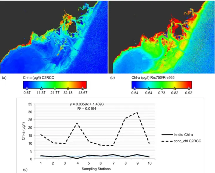
705 nm/665 nm. Therefore, NIR/Red ratio product C2RCC was selected to map Chl-a in the submerged zone of the estuarine system. by following equation (Figure 10(b)).
[
]
(
)
Chl-a= Rrs705 Rrs665 −1.103 0.1072 (3) Figure 10(a) shows the spatial distribution of Chl-a (conc_chl) C2RCC, High Chl-concentrations coincided in the shallow water area associated with seagrass with values that exceed 45 µg/l. The result of this product shows an overestima-tion of the concentraoverestima-tions Chl-a, particularly in shallow water, compared to the output map of the algorithm applied (Equation (3)) in concentrations closer to the Chl- a in situ measurement (Figure 10(b)).
Figure 10. (a) Spatial distribution of the Chl-a (conc_chl) C2RCC, (b) Chl-a (NIR/Red) ratio (Equation (3)) and (c) Correlation between conc_chl C2RCC, and data and chlorophyll a measured from water samples in situ Chl-a.
DOI: 10.4236/ijg.2020.1110035 721 International Journal of Geosciences
A relationship between in situ data Chl-a and Conc_chl C2RCC product as a function of the measurement station (Figure 10(c)) shows us the over-estimation of chlorophyll concentrations throughout the region of the Kneiss islands and the unreliability of the Chl-a algorithm C2RCC for these types of coastal area.
3.2.3. Estimation of TU Using Sentinel 2A Data
Linear regression coefficients were computed to search for a better channel for estimating in situ TU data Figures 11(a)-(f). The water-leaving radiance reflec-tance for the 665 nm band showed the best regression coefficient with the in situ TU data with an R2 value of 0.70. Similar results were reported [7] [8] [19]
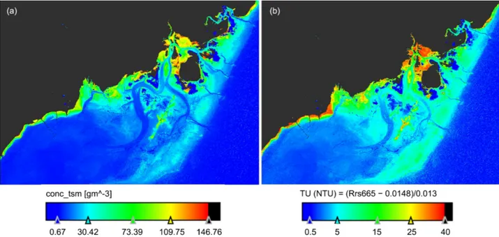
showing a good agreement between field and modeled TU for the analyzed sites. The product conc_TSM C2RCC also shows a good relationship with the Turbid-ity TU data measured from water sample with an R2 value of 0.62 (Figure 11(g)
and Figure 12(a)).
(
)
TU= Rrs665 0.014 0.013− (4) despite the overestimation of values of TU. The following empirical relation (Equation (4)) was deduced for the quantification of turbidity in the Kneiss Isl-ands from the Sentinel 2A data (Figure 12(b)) shows us close to that measured values at sea.
4. Discussion and Conclusions
Kneiss Islands is a very complex study environment due to morphological, hy-drodynamic, and biological particularities. Mainly because of the influence of semi-diurnal type tides with amplitudes reaching up to 2 m, we used two types of high-resolution sensors (30 m, 20 m, 10 m) for studying optical properties (Chl-a) and water quality (TU). In the absence of reflectance data at sea in Tuni-sia, we have developed an indirect method of extracting and validating Chl-a and TU satellite data. We used the reflectance or reflectance ratios at different wave-lengths and compared a reduced set of in situ data for Chl-a and TU in µg/L, and NTU is obtained concurrently to the images (18 in 2009 and 10 in 2017). The best linear regressions for the calculation and mapping of Chl-a and TU from satellite data are summarized in Table 2 and Table 3. For a measured chloro-phyll with a range of 0.5 - 4.7 µg/L, Chl-a EO1 offset is 0 while it is 1 for Sentinel 2. For a measured turbidity range of 0 - 38 NTU, offset is 11.48 for TU EO1 and 1 for TU S2A. Large offsets in these linear regressions indicate the influence of bottom reflectance.
Several oceanographic studies, biogeochemical, fisheries features [54], am-phipods [55], faunal analysis [56] were carried out in the Gulf of Gabes and Kneiss islands. The results are temporary and not continuous over time, which is why the extraction and generation of an algorithm for the continuous quantifi-cation of water quality data is a necessity in these types of environment. Data and relationships extracted from Sentinel S2A can effectively help us quantify seawater quality. According to our work, the Sentinel 2 radiometric data with a
DOI: 10.4236/ijg.2020.1110035 722 International Journal of Geosciences Figure 11. Cross relationships of in situ TU to Remote sensing reflectance C2RCC 443 nm, 490 nm, 560 nm, 665 nm, 705 nm, 740 nm (a), (b), (c), (d), (e), (f),correlation between conc-TSM C2RCC product and TU measured from water sample (g).
DOI: 10.4236/ijg.2020.1110035 723 International Journal of Geosciences Figure 12. (a) Spatial distribution of the total suspended matter (conc_tsm) C2RCC, (b) TU(NTU) (Equation (4)).
Table 2. Satellite CHL-a Validation based on in situ data.
Sensor λ (nm) Equation CHL-a (µg/L) Regression Coefficient (R2) Spatial resolution EO1 457 - 528 Rrs457 Rr Chl-a 0. s528 005 = 0.57 30 m Sentinel 2 705 - 665 Chl-a=
(
[Rrs705 Rrs665]−1.103 0.1072)
0.72 20 m Table 3. Satellite TU Validation based on in situ data.Sensor λ (nm) Equation TU (NTU) Coefficient (RRegression 2)
Spatial resolution EO1 550 TU = 0.218 (Rrs550) + 11.248 0.63 30 m Sentinel 2 665 TU = (Rrs665 − 0.014)/0.013 0.70 20 m
spatial resolution of 10 m and 20 m gave us the best results for the study area for a slice of water greater than 50 cm with coefficients of determination greater than 0.68 for both TU and Chl-a. Indeed, the reflection of the seabed was identi-fied by very high values of chlorophyll concentration and turbidity. The Chl-a and TU predicted in these areas using EO1 and S2A data clearly delimit the lo-calities where we might have doubtful results. Moreover, we developed a region of interest via 2D scatter plot between 665 nm and 865 nm bands to identify and mask the position of pixels of tidal swing area before processing to eliminate the effect of background reflections at the moment of the satellite passage.
Despite the fineness of the spectral bands of EO1 (we could use only 39 bands among the available 220 bands), the reflectance has a very low radiometric
qual-DOI: 10.4236/ijg.2020.1110035 724 International Journal of Geosciences
ity, especially in aquatic environments. This can explain the lower coefficients of determination for the prediction of TU and Chl-a using the EO1 (R2 = 0.57 -
0.63). Table 2 and Table 3 show that wavelengths of the best reflectance or ref-lectance ratios differ between Hyperion EO1 and Sentinel 2A. Nevertheless, the ones used for Chl-a (457 nm/528 nm for EO1 and 705 nm/665 nm for Sentinel 2) and for TU (550 nm for EO1 and 665 nm for Sentinel 2) are remarkably simi-lar to those used in other reported studies.
Acknowledgements
This study was funded by GEOMAG Laboratory University of Manouba in col-laboration with Applied Hydrosciences Unit at the Higher Institute of Sciences and Techniques of Water of Gabès ISSTEG and PRODIG lab as part of the project on the ecosystems of the Kneiss islands and Leben basin. We thank GreenLab for their professionalism, and Sentinel2 Scientific data Hub and NASA GSFS team distribution
Funding
This work has received financial support from the LabEx DynamiTe (ANR-11-LABX-0046), as part of the “Investissements d’Avenir” program.
Conflicts of Interest
The authors declare no conflicts of interest regarding the publication of this pa-per.
References
[1] Tassan, S. (1994) Local Algorithms Using SeaWiFS Data for the Retrieval of Phy-toplankton, Pigments, Suspended Sediment, and Yellow Substance in Coastal Wa-ters. Applied Optics, 33, 2369-2378. https://doi.org/10.1364/AO.33.002369
[2] Doxaran, D., Froidefond, J.-M., Lavender, S. and Castaing, P. (2002) Spectral Sig-nature of Highly Turbid Waters. Application with SPOT Data to Quantify Sus-pended Particulate Matter. Remote Sensing of Environment, 81, 149-161.
https://doi.org/10.1016/S0034-4257(01)00341-8
[3] Lee, Z., Casey, B., Arnone, R., Weidemann, A., Parsons, R., Montes, M.J., Gao, B.C., Goode, W., Davis, C.O. and Dye, J. (2007) Water and Bottom Properties of a Coast-al Environment Derived from Hyperion Data Measured from the EO-1 Spacecraft Platform. Journal of Applied Remote Sensing, 1, 011502.
https://doi.org/10.1117/1.2822610
[4] Brando, V.E. and Phinn, S.R. (2007) Coastal Aquatic Remote Sensing Applications for Environmental Monitoring and Management. Journal of Applied Remote Sens-ing, 1, 011599. https://doi.org/10.1117/1.2835115
[5] Nechad, B., Ruddick, K.G. and Neukermans, G. (2009) Calibration and Validation of a Generic Multisensor Algorithm for Mapping of Turbidity in Coastal Waters.
Proceedings of SPIE “Remote Sensing of the Ocean, Sea Ice, and Large Water Re-gions”, Vol. 7473, Berlin, 31 August 2009, 74730H.
DOI: 10.4236/ijg.2020.1110035 725 International Journal of Geosciences [6] Traganos, D., Cerra, D. and Reinartz, P. (2017) Cubesat-Derived Detection of Sea-grasses Using Planet Imagery Following Unmixing-Based Denoising: Is Small the Next Big? International Archives of the Photogrammetry, Remote Sensing & Spatial Information Sciences, 42, 283-287.
https://doi.org/10.5194/isprs-archives-XLII-1-W1-283-2017
[7] Nechad, B., Ruddick, K.G. and Park, Y. (2010) Calibration and Validation of a Ge-neric Multisensor Algorithm for Mapping of Total Suspended Matter in Turbid Waters. Remote Sensing of Environment, 114, 854-866.
https://doi.org/10.1016/j.rse.2009.11.022
[8] Katlane, R., Nechad, B., Ruddick, K. and Zargouni, F. (2011) Optical Remote Sens-ing of Turbidity and Total Suspended Matter in the Gulf of Gabes. Arabian Journal of Geosciences, 6, 1527-1535. https://doi.org/10.1007/s12517-011-0438-9
[9] Vermote, E.F., Tanré, D., Deuzé, J.L., Herman, M. and Morcrette, J.-J. (1997) Second Simulation of the Satellite Signal in the Solar Spectrum, 6S: An Overview,
IEEE Transactions on Geoscience and Remote Sensing, 35, 675-686. https://doi.org/10.1109/36.581987
[10] Gordon, H.R., Brown, O.B., Evans, R.H., Brown, J.W., Smith, R.C., Baker, K.S. and Clark, D.K. (1998) A Semi-Analytic Radiance Model of Ocean Color. Journal of Geophysical Research: Atmospheres, 93, 10909-10924.
https://doi.org/10.1029/JD093iD09p10909
[11] O’Reilly, J.E. (2000) Ocean Color Chlorophyll-a Algorithm for SeaWiFS, OC2, and OC4: SeaWiFS Postlaunch Technical Report Series. In: Hooker, S.B. and Firestone, R., Eds., Volume 11, SeaWiFS Postlaunch Calibration and Validation Analyses Ver-sion 4, Part 3, NASA Goddard Space Flight Center, Greenbelt, 9-23.
[12] Gohin, F., Druon, J.N. and Lampert, L. (2002) A Five Channel Chlorophyll Algo-rithm Applied to SeaWifs Data Processed by SeaDas in Coastal Waters. Interna-tional Journal of Remote Sensing, 23, 1639-1661.
https://doi.org/10.1080/01431160110071879
[13] Maritorena, S., Siegel, D.A. and Peterson, A.R. (2002) Optimization of a Semi Ana-lytical Ocean Color Model for Global-Scale Applications. Applied Optics, 41, 2705-2714. https://doi.org/10.1364/AO.41.002705
[14] Han, L. and Jordan, K.J. (2005) Estimating and Mapping Chlorophyll-a Concentra-tion in Pensacola Bay, Florida Using Landsat ETM+ Data. International Journal of Remote Sensing, 26, 5245-5254. https://doi.org/10.1080/01431160500219182 [15] Griffin, M.K., Su May, H., Burke, H.K., Orloff, S.M. and Upham, C.A. (2005)
Ex-amples of EO-1 Hyperion Data Analysis. Lincoln Laboratory Journal, 15, No. 2. [16] Doxaran, D., Castaing, P. and Lavender, S.J. (2006) Monitoring the Maximum
Tur-bidity Zone and Detecting Finescale TurTur-bidity Features in the Gironde Estuary Us-ing High Spatial Resolution Satellite Sensor (SPOT HRV, Landsat ETM+) Data. In-ternational Journal of Remote Sensing, 27, 2303-2321.
https://doi.org/10.1080/01431160500396865
[17] Babin, M., Stramski, D., Ferrari, G.M., Claustre, H., Bricaud, A. and Obolenski, G. (2003) Variations in the Light Absorption Coefficients of Phytoplankton, Non-Algal Particles, and Dissolved Organic Matter in Coastal Waters around Europe. Journal of Geophysical Research: Oceans, 108, No. C7.
https://doi.org/10.1029/2001JC000882
[18] Zhu, W., Tian, Y.Q., Yu, Q. and Becker, B.L. (2013) Using Hyperion Imagery to Monitor the Spatial and Temporal Distribution of Colored Dissolved Organic Mat-ter in Estuarine and Coastal Regions. Remote Sensing of Environment, 134,
DOI: 10.4236/ijg.2020.1110035 726 International Journal of Geosciences 342-354. https://doi.org/10.1016/j.rse.2013.03.009
[19] Dogliotti, A.I., Ruddick, K., Nechad, B., Doxaran, D. and Knaeps, E. (2015) A Single Algorithm to Retrieve Turbidity from Remotely-Sensed Data in All Coastal and Es-tuarine Waters. Remote Sensing of Environment, 156, 157-168.
https://doi.org/10.1016/j.rse.2014.09.020
[20] Hedley, J.D., Roelfsema, C.M., Phinn, S.R. and Mumby P.J. (2012) Environmental and Sensor Limitations in Optical Remote Sensing of Coral Reefs: Implications for Monitoring and Sensor Design. Remote Sensing, 4, 271-302.
https://doi.org/10.3390/rs4010271
[21] Fischer, A.M., Pang, D., Kidd, I.M. and Moreno-Madriñán, M.J. (2017) Spa-tio-Temporal Variability in a Turbid and Dynamic Tidal Estuarine Environment (Tasmania, Australia): An Assessment of MODIS Band 1 Reflectance. ISPRS Inter-national Journal of Geo-Information, 6, 320.
https://doi.org/10.3390/ijgi6110320
[22] Vanhellemont, Q. and Ruddick, K. (2016) ACOLITE for Sentinel-2: Aquatic Appli-cations of MSI Imagery. Proceedings of the 2016 ESA Living Planet Symposium, Prague, 9-13 May 2016, ESA Special Publication SP-740.
[23] Ansper, A. and Alikas, K. (2019) Retrieval of Chlorophyll a from Sentinel-2 MSI Data for the European Union Water Framework Directive Reporting Purposes.
Remote Sensing, 11, 64. https://doi.org/10.3390/rs11010064
[24] Uwe, M.W., Jerome, L., Rudolf, R., Ferran, G. and Marc, N. (2013) Sentinel-2 Level 2a Prototype Processor: Architecture, Algorithms and First Results. Proceedings of the ESA Living Planet Symposium, ESA SP-722, 3-10.
[25] Toming, K., Kutser, T., Laas, A., Sepp, M., Paavel, B. and Nõges, T. (2016) First Ex-periences in Mapping Lake Water Quality Parameters with Sentinel-2 MSI Imagery.
Remote Sensing, 8, 640. https://doi.org/10.3390/rs8080640
[26] Steinmetz, F., Deschamps, P.-Y. and Ramon, D. (2011) Atmospheric Correction in Presence of Sun Glint: Application to MERIS. Optics Express, 19, 9783-9800. https://doi.org/10.1364/OE.19.009783
[27] Mobley, C.D., Sundman, L., Zhang, H. and Voss, K.J. (2000) Light and Water. Ef-fects of Optically Shallow Bottoms on Water-Leaving Radiances, Ocean Optics XV, Monte Carlo.
[28] Zaneveld, J.R.V. and Boss, E. (2003) The Influence of Bottom Morphology on Ref-lectance: Theory and Two-Dimensional Geometry Model. Limnology and Oceano-graphy, 48, part 2. https://doi.org/10.4319/lo.2003.48.1_part_2.0374
[29] Jaquet, J.M., Tassan, S., Barale, V. and Sarbaji, M. (1999) Bathymetric and Bottom Effects on CZCS Chlorophyll-Like Pigment Estimation: Data from the Kerkennah Shelf (Tunisia). International Journal of Remote Sensing, 20, 1343-1362.
https://doi.org/10.1080/014311699212777
[30] Shimi, M. (1980) Etude sédimentologique de la région de Kneiss (Golfe de Gabès, Tunisie). Thèse de Spécialité, Université Paris Sud, Paris.
[31] Kneiss Islands (1993) Forestry Commission at the Ministry of Agriculture. Law No. 88-20.
[32] HP (Hydrotecnica Portuguesa) (1995) Etude générale pour la protection du littoral Tunisien. Rapport.
[33] Oueslati, A., Paskoff, R., Slim, H. and Trousset, P. (1992) Les îles Kneiss et le monastère de Fulgence de Ruspe. Antiquités Africaines, 28, 223-247.
DOI: 10.4236/ijg.2020.1110035 727 International Journal of Geosciences [34] Bali, M. and Gueddari, M. (2011) Les chenaux de marée autour des îles de Kneiss,
Tunisie: Sédimentologie et évolution. Hydrological Sciences Journal, 56, 498-506. https://doi.org/10.1080/02626667.2011.563240
[35] Guillaumont, B. (1992) Etude des masses d’eaux du Golfe de Gabès par télédétection. Rapport final sur la pollution marine dans le Golfe de Gabès. Rapport interne, Centre National de Télédétection, ANPE.
[36] Gueddari, M. and Oueslati, A. (2002) Le site de Kneiss, Tunisie: geomorphologie et aptitudes à l’aménagement. In: Scapini, F., Ed., Recherche de Base pour une Gestion Durable des Ecosystèmes Sensibles Côtiers de la Méditerranée, Istituto Agronomico per l’Oltremare, Italie, 63-71.
[37] Trousset, P. (2008) Kneiss. In: Chaker, S., Kirtēsii-Lutte, Aix-en-Provence, Edisud, 28-29, 4251-4254. http://encyclopedieberbere.revues.org/99
https://doi.org/10.4000/encyclopedieberbere.99
[38] Oueslati, A. (1993) Les côtes de la Tunisie: Géomorphologie et environnement et aptitudes à l’aménagement. Faculté des Sciences Humaines et Sociales de Tunisie, Tunis.
[39] Ghribi, R., Sghari, A. and Bouaziz, S. (2006) Le bassin de l’oued Ouadrane (Tunisie méridionale): Evolution géomorphologique et néotectonique. Notes du Service Géologique de Tunisie, 74, 77-97.
[40] Suhet ESA Standard Document (2013) Issue 1 Rev 2 Sentinel2 User Hand Book. [41] Pahlevan, N., Sarkar, S., Franz, B.A., Balasubramanian, S.V. and He, J. (2017)
Sen-tinel-2 Multispectral Instrument (MSI) Data Processing for Aquatic Science Appli-cations: Demonstrations and Validations. Remote Sensing of Environment, 201, 47-56. https://doi.org/10.1016/j.rse.2017.08.033
[42] Toming, K., Arst, H., Paavel, B., Laas, A. and Nõges, T. (2009) Spatial and Temporal Variations in Coloured Dissolved Organic Matter in Large and Shallow Estonian Waterbodies. Boreal Environment Research, 14, 959-970.
[43] Su May, H., Hsiao-Hua, K., Burke Seth Orloff, M. and Griffin, K. (2003) Examples of EO-1 Data Analysis. Proceedings of SPIE, Algorithms and Technologies for Mul-tispectral, Hyperspectral, and Ultraspectral Imagery IX, Orlando, 23 September 2003, Vol. 5093.
[44] Tilstone, G. and Moore, G., Eds. (2002) REVAMP Regional Validation of MERIS Chlorophyll Products in North Sea Coastal Waters: Protocols Document.
[45] Griffin, M.K., Su May, H., Burke, H.K., Orloff, S.M. and Upham, C.A. (2005) Ex-amples of EO-1 Hyperion Data Analysis. Lincoln Laboratory Journal, 15, No. 2. [46] Gao, B.C., Montes, M.J., Ahmad, Z. and Davis, C.O. (2000) Atmospheric Correction
Algorithm for Hyperspectral Remote Sensing of Ocean Color from Space. Applied Optics, 39, 887-896. https://doi.org/10.1364/AO.39.000887
[47] Dupouy, C., Neveux, J., Ouillon, S., Frouin, R., Murakami, H., Hochard, S. and Dirberg, G. (2010) Inherent Optical Properties and Satellite Retrieval of Chlorophyll Concentration in the Lagoon and Open Ocean Waters of New Caledonia. Marine Pollution Bulletin, 61, 503-518. https://doi.org/10.1016/j.marpolbul.2010.06.039 [48] Katlane, R., Dupouy, C. and Zargouni, F. (2012) Chlorophyll and Turbidity
Con-centrations Deduced from MODIS as an Index of Water Quality of the Gulf of Gabes in 2009. Revue Télédétection, 11, 263-271.
[49] Blondeau-Patissier, D., Gower, J.F., Dekker, A.G., Phinn, S.R. and Brando, V.E. (2014) Review of Ocean Color Remote Sensing Methods and Statistical Techniques for the Detection, Mapping and Analysis of Phytoplankton Blooms in Coastal and
DOI: 10.4236/ijg.2020.1110035 728 International Journal of Geosciences Open Oceans. Progress in Oceanography, 123, 123-144.
https://doi.org/10.1016/j.pocean.2013.12.008
[50] Dorji, P. and Fearns, P. (2016) Quantitative Comparison of Total Suspended Sedi-ment Algorithms: A Case Study of the Last Decade for MODIS and Landsat-Based Sensors. Remote Sensing, 8, 810. https://doi.org/10.3390/rs8100810
[51] Brando, V.E. and Dekker, A.G. (2003) Satellite Hyperspectral Remote Sensing for Estimating Estuarine and Coastal Water Quality. IEEE Transactions on Geoscience and Remote Sensing, 41, 1378-1387. https://doi.org/10.1109/TGRS.2003.812907 [52] Sakuno, Y., Yajima, H., Yoshioka, Y., Sugahara, S., Mohamed, A.M., Abd Elbasit
Elh, A. and Chirima, J.G. (2018) Evaluation of Unified Algorithms for Remote Sensing of Chlorophyll-a and Turbidity in Lake Shinji and Lake Nakaumi of Japan and the Vaal Dam Reservoir, of South Africa under Eutrophic and Ultra-Turbid Conditions. Water, 10, 618. https://doi.org/10.3390/w10050618
[53] Soomets, T., Uudeberg, K., Jakovels, D., Brauns, A., Zagars, M. and Kutser, T. (2020) Validation and Comparison of Water Quality Products in Baltic Lakes Using Sentinel-2 MSI and Sentinel-3 OLCI Data. Sensors, 20, 742.
https://doi.org/10.3390/s20030742
[54] Béjaoui, B., Ben Ismail, S., Othmani, A., Ben Abdallah-Ben Hadj Hamida, O., Che-valier, C., Feki-Sahnoun, W., Harzallah, A., Ben Hadj Hamida, N., Bouaziz, R., Da-hech, S., Diaz, F., Tounsi, K., Sammari, C., Pagano, M. and Bel Hassen, M. (2019) Synthesis Review of the Gulf of Gabes (Eastern Mediterranean Sea, Tunisia): Mor-phological, Climatic, Physical Oceanographic, Biogeochemical and Fisheries Fea-tures. Estuarine, Coastal and Shelf Science, 219, 395-408.
https://doi.org/10.1016/j.ecss.2019.01.006
[55] Fersi, A., Dauvin, J.C., Pezy, J.P. and Neifar, L. (2018) Amphipods from Tidal Channels of the Gulf of Gabès (Central Mediterranean Sea). Mediterranean Marine Science, 19, 430-443. https://doi.org/10.12681/mms.15913
[56] Mosbahi, N., Boudaya, L., Neifar, L. and Dauvin, J.-C. (2020) Do Intertidal Zostera noltei Meadows Represent a Favourable Habitat for Amphipods? The Case of the Kneiss Islands (Gulf of Gabès: Central Mediterranean Sea). Marine Ecology, 41, e12589. https://doi.org/10.1111/maec.12589