HAL Id: hal-02336285
https://hal.archives-ouvertes.fr/hal-02336285
Submitted on 28 Oct 2019HAL is a multi-disciplinary open access archive for the deposit and dissemination of sci-entific research documents, whether they are pub-lished or not. The documents may come from teaching and research institutions in France or abroad, or from public or private research centers.
L’archive ouverte pluridisciplinaire HAL, est destinée au dépôt et à la diffusion de documents scientifiques de niveau recherche, publiés ou non, émanant des établissements d’enseignement et de recherche français ou étrangers, des laboratoires publics ou privés.
Merging velocity measurements and modeling to
improve understanding of tidal stream resource in
Alderney Race.
Maxime Thiébaut, Alexei Sentchev, Pascal Bailly Du Bois
To cite this version:
Maxime Thiébaut, Alexei Sentchev, Pascal Bailly Du Bois. Merging velocity measurements and modeling to improve understanding of tidal stream resource in Alderney Race.. Energy, Elsevier, 2019, 178, pp.460-470. �10.1016/j.energy.2019.04.171�. �hal-02336285�
Merging velocity measurements and modeling to improve understanding of tidal stream resource in Alderney Race
Maxime Thiébaut1,2, Alexei Sentchev*1 and Pascal Bailly du Bois3
(1) Univ. Littoral Côte d’Opale, Univ. Lille, CNRS, UMR 8187, LOG, Laboratoire d’Océanologie et de Géosciences, Wimereux, France
(2) France Énergies Marines, Technopôle Brest-Iroise, Batîment Cap Océan, 525 Avenue de Rochon, Plouzané, France
(3) IRSN/DEI/SECRE/LRC, Institut de Radioprotection et de Sûreté Nucléaire, Direction de l Environnement et de l Intervention, Laboratoire de Radioécologie de Cherbourg Octeville,
France
(*) Corresponding author: [email protected] Phone : +33 3 21 99 64 17 Fax : + 33 3 21 99 64 01
Abstract
Tidal circulation and tidal stream resource in Aldemey Race (Raz Blanchard) were assessed by using a towed acoustic Doppler current profiler (ADCP) system and tidal modeling. Optimal Interpolation (OI) was applied to process the underway velocity measurements recorded at neap tide flood and ebb flow. The interpolation technique allows reconstructing space-time evolution of the velocity field within the domain during surveying periods. The method employs velocity covariances derived from numerical simulations by a 2D hydrodynamic model MARS. Model covariances are utilized by the OI algorithm to obtain the most likely evolution of the velocity field under the constraints provided by the ADCP observations and their error statistics. The resulting velocity fields were used for assessing the tidal stream resource at site. The largest overall difference between the kinetic power density derived from simulated and interpolated velocity fields was found for ebb tide. Model simulations constrained by velocity measurements demonstrated a significant (up to 30%) decrease of power available in the flow. A significant change in spatial pattern of power density distribution was also identified. It is demonstrated that by merging high resolution velocity measurements at tidal energy site with modeling the tidal stream potential estimation becomes more accurate.
Keywords: ADCP measurements; Alderney Race; Optimal Interpolation; Tidal model; Tidal stream resource.
1. Introduction
Tidal energy conversion by in-stream turbines installed at nearshore macro-tidal sites is an attractive method of electric power production with zero carbon emission. For high efficiency and commercial viability of projects, the tidal energy convertors (TEC) require large current velocities, typically spring tide velocities in excess of 2.5 m/s (Lewis et al., 2015). Regions of such high-tidal current speeds are sparse, and are typically the result of topographic flow amplification. A fast moving tide passing through a bathymetry constriction can result in a tidal race (extremely strong current). Very large current speeds (up to 5 m/s) have been encountered in certain specific locations along the UK and French coasts. The Channel Isles region located west of the Cotentin Peninsula in Normandy, France, is one of these areas. Several sites of medium to high potential were identified there (Coles et al., 2017), with the highest potential found in Alderney Race (Bahaj and Myers, 2004; Myers and Bahaj, 2005; Coles et al., 2017, Guillou et al., 2018). Using Telemac 2D model of the English Channel, with an enhanced spatial and temporal resolution, Coles et al., (2017) obtained more reliable quantification of the tidal stream resource in comparison with previous regional scale studies. The authors estimated that the maximum power that can be extracted in Alderney Race is 5.1 GW which is 35% more than a previous estimate for the Pentland Firth, UK (Draper et al., 2014), and only 10% less than the maximum power that can be extracted in the Minas Passage (Bay of Fundy), Canada (Walters et al., 2013). Compared to sites considered to have the world’s largest tidal stream resource, e.g., Minas Passage and Pentland Firth, the theoretical potential in Alderney Race appears also very large and economic issues of tidal energy conversion are sought to be very important.
In order to optimize TEC performance, an accurate assessment of the available tidal energy resource at high spatial and temporal resolution is required. Although a relatively good assessment of the local hydrodynamics and tidal stream resource in Alderney Race, provided by numerous numerical studies, is reliable (e.g. Bahaj and Myers, 2004; Bailly du Bois et al., 2012; Thiébot et al., 2015; Coles et al., 2017; Guillou et al., 2018), high quality tidal stream measurements in this area are scarce. This is due to extreme difficulties of in situ data acquisition. However, direct measurements are essential in highly energetic tidal environment such as Alderney Race to address the commercial viability of tidal energy conversion projects.
Over the last decade, standardized methods of field data acquisition for resource characterization at tidal energy sites have been proposed (e.g., Legrand, 2009; Venugopal et al., 2011). Current measurements by acoustic Doppler current profilers (ADCPs) are routinely used to directly characterize the tidal flow. A bottom-mounted ADCP is often deployed for measuring temporal variations, while a vessel-mounted ADCP can measure spatial variations. However, deployment and recovery of ADCPs at tidal energy sites with extreme current and wave climate is difficult. In this case, underway velocity
measurements offer a more practical alternative to fixed point observations. Although the vessel-mounted ADCPs are in use now for more than twenty-five years (e.g., Simpson et al., 1990; Geyer and Signell, 1990; Vennell, 1994; Goddijn-Murphy et al., 2013; Sentchev and Yaremchuk, 2016), their efficiency for tidal energy resource assessment was demonstrated only recently.
Experimental works mentioned above employed repeated circuits in which the vessel follows the same tracks several times during a complete tidal cycle. Thus, velocity profiles are recorded with sufficient frequency to resolve spatial irregularities of the flow field. However, due to wide gaps along the vessel tracks, measurements are required to be interpolated. Since underway ADCP measurements contain information on both spatial and temporal variations of tidal currents, these variations need to be separated from each other. For this purpose, a number of techniques have been tested to date. Geyer and Signell (1990), Simpson et al. (1990), Vennell (1994) separated spatial and temporal components of the flow by spatially binned ADCP velocity measurements from each track. The time series of velocities for each bin were analyzed using conventional tidal analysis techniques to yield harmonics coefficient of the principal tidal constituents (e.g., M2, S2, N2) for the bins. However, such a technique generates spatial noise in the calculation of harmonic coefficients due to independent tidal analysis in adjacent bins.
Vennell (2006) used a biharmonic spline tidal analysis technique, for space-time interpolation of velocity data recorded by ADCP in a narrow (600-m wide) tidal channel. This study revealed the high sensitivity of the method to the amount of data and its spatial distribution. Vennell and Beatson (2009), developed a 2D divergence-free spatial interpolator that ensures mass conservation and provides more realistic estimates of the depth-averaged velocities. MacMahan et al. (2012) applied a similar technique for interpolating noisy data from an ADCP mounted on an underwater vehicle. Using vessel-mounted ADCP surveys, Goddijn-Murphy et al. (2013), Polagye and Thomson (2013) documented fine scale velocity variations caused by tidal flow interaction with land and islands. However, the rapid change of the tidal flow during surveying period tends to induce errors in the velocity map interpretation. Goddijn- Murphy et al. (2013) showed that if a tidal model provides a reasonable estimate of flow field, an output of the model could be utilized to project the transect data to a fixed (central) time of the survey. Using a 2D model POLPRED (Proudman Oceanographic Laboratory Model), they performed a reasonably accurate synchronization of the velocity data to the mid-survey time. However, a relatively coarse resolution of the model did not allow assessing smaller-scale features of the tidal flow, such as eddies, cross currents, and jets because temporal resolution of the model (10 min) appeared to be close to the limit required for resolving rapid evolution of these features. More recently, Sentchev and Yaremchuk (2016) used the Optimal Interpolation (OI) technique for reconstructing space-time evolution of the velocity field derived from towed ADCP surveys in the Boulogne harbor (English Channel). Their approach, which combines underway velocity measurements and modeling, provides a considerable improvement in
reconstructing the tidal dynamics compared to what the model can do alone and offers a real opportunity for short-term monitoring of coastal currents.
This study aims to provide a methodology for estimating the tidal stream potential at tidal energy site in the most accurate way by merging underway current velocity measurements with model outputs. In this work, considered as an extension of the previous study by Sentchev and Yaremchuk (2016), we further developed and applied the OI technique to interpolate underway velocity measurements performed with a towed (not vessel-mounted) ADCP in Alderney Race. Velocity profiles, recorded continuously along transects during sufficiently long periods of the tidal cycle (up to 5 hours), allowed detailed characterization of space-time variability of the flow and comparison with a 2D circulation model output. Observed current velocities were then synchronized in time using the statistics from the model MARS (Model for Applications on Regional Scale) configured for high-resolution simulations in the surveyed area. The resulting velocity fields were used for assessing the tidal stream resource at site during neap tide.
2. Data and methods 2.1 Study site
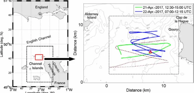
Velocity measurements presented here were performed in the eastern (French) sector of Alderney Race located to the west of the Cotentin Peninsula in Normandy, France (Fig. 1). The surveyed area is approximately 10 x 7 km square with water depth less than 50 m throughout the domain. The sea surface height (SSH) in Goury, a small harbor close to the surveying area (see Fig. 1 for location) exhibits a wide range of tidal variations (2.5-7m) depending on the tidal stage. According to modeling results, tidal variations of SSH and currents are predominantly semi-diurnal and globally symmetric. On average, current velocities are higher during ebb tide than during flood tide (Fig. 2). Peak flood and ebb tidal velocities occur at high and low water respectively with slack water at mid-tide. The tidal current dynamics is thus referred to as progressive wave system. Tidal wave propagates northward during flood flow which lasts for 6 hours and then changes a direction to southward for the next 6 hours.
Current velocities vary considerably throughout the Race. At mean tide, the maximum tidal current speed, up to 3.5 m/s, is observed at the eastern side of Alderney Race (Bahaj and Myers, 2004). Such strength of the current is due to the local acceleration of the tidal flow between Alderney Island and Cap de la Hague (Fig. 1). Spring tidal flow is extremely powerful. According to modeling, the highest velocities (more than 5 m/s) are found again in the eastern sector of Alderney Race, in a large area extending up to 5 km off the French coast (e.g. Thiébot et al., 2015; Coles et al., 2017).
2.2 Underway velocity measurements
High-resolution velocity measurements were performed in Aldemey Race using an experimental platform, carrying a broadband ADCP (600 kHz Teledyne RDI WorkHorse Sentinel) and towed by the R/V “Thalia”. The deep-towed depressor platform (Dynalest) is 2.4-m long and 1.6-m wide and was developed at the National Institute for Radiological Protection and Nuclear Safety (IRSN). It is composed, in the rear part, of an adjustable tail plane (with two vertical stabilization wings) and a main wing in the front part, connected together by two girders (Fig. 3). The wing assures the maximum stability of the platform for a wide range of operational speeds (1-5 m/s) without generating tilts. A risk of cavitation could appear at speeds above 7 m/s. The Dynalest was first designed to obtain a maximum vertical strength for deployment of in-depth sampling systems (more than 65 m). The maximum operating depth can be changed by modifying the wing surface-area (chord and width dimensions). The use of Dynalest during surveys reported here targeted to maintain the ADCP in the most stable conditions, under the water surface and below the influence of surface waves. More details about the Dynalest can be found in Bailly du Bois et al. (2014).
During the surveys, the towed ADCP was located roughly 8.5 m below the water surface with the third beam aligned along the platform’s centerline. The bin size was set to 1 m. The velocity profiles were recorded from 10 m depth to the sea bottom. The ADCP was set to operate at the pinging rate of 1 Hz. Each ping for velocity was composed of three sub-pings averaged within 1-s interval, providing velocity error of 0.04 m/s. Single-ping bottom tracking was enabled to correct for boat’s movement, and the recorded velocities formed a current vector in the fixed frame relative to the bottom. The vessel’s speed was typically 2-3 m/s for the majority of the tracks. The ADCP data were merged with navigation data provided by onboard GPS system also operating at 1 Hz.
Underway velocity measurements were performed during neap tide, under very weak wind (mean speed 2 m/s, max speed 5 m/s) and low waves (Hs < 0.4 m). Neap tide conditions were specifically targeted as the fieldworks were devoted principally to the deployment of three bottom-mounted ADCPs and drifting buoys in the study area. The availability of the R/V “Thalia”, between different steps of the sea trials, allowed to carry out a total of four towed ADCP surveys during different stages of the tidal cycle (Fig. 2). The results of the two longest surveys, S3 and S4, separated by two tidal cycles are presented in this paper. Survey 3 was performed on April 21, 2017 at 12:30-15:00 UTC, before reaching high water (HW) in Goury: from HW-2.5 hours to HW. Survey S4 was performed the next day, on April 22, at 07:00-12:15 UTC, during the ebb flow and lasted slightly more than 5 hours: from low water (LW) - 3 hours to LW+2.25 hours. Shorter surveys (S1 and S2) provided complementary data which were used for comparison with the model output and misfit estimation. Current velocities recorded by ADCP were corrected for boat motion and averaged within 1 minute intervals. GPS coordinates were also sub-sampled
every minute, so that the distance between the thinned along-track data points varied within 120-180 m, depending on the towing speed. Velocities were then vertically averaged for comparison with the model output. Survey tracks and measurement locations are shown in Fig. 1 (right panel).
The deployment of one of three 600 kHz bottom-mounted RDI ADCP in the surveying area allowed to supplement underway velocity measurements by tidal current observations at a fixed point (red triangle in Fig. 1). Velocities were recorded from April 21 to June 03, 2017 every 5 min at 1 m vertical resolution starting from 2 m above the bottom. The mean depth was 45 m and velocity values in the surface 7-8 m thick layer, were removed from analysis because of signal contamination by surface waves.
2.3 Optimal interpolation: basic formulation
Optimal Interpolation (OI) is a commonly used and powerful method of objective analysis of observations. OI provides estimation of the spatial distribution of a physical quantity at a given time through a linear combination of the available data. This technique, pioneered by Gandin (1963) was widely adopted in geosciences (Bretherton et al. 1976; Thiébaux and Pedder 1987; Wunsch, 1996; Sentchev and Yaremchuk 2016).
The OI technique can be easily extended to include time dimension by using the space-time correlation fonctions. In this approach, the optimal correction to the evolution of a background vector field um(x,t) defined on a regular (model) grid is represented by a linear combination of the weighted differences between the background trajectory and the observed velocities. The weights at are chosen so as to minimize the mean square difference between observations u,* and the background field values um, interpolated into the space-time locations of the observations by the linear operator H,, projecting gridded velocity values onto the i-th observation point from the apexes of the enveloping grid cell:
Ju = <[Um + ^ fo (H;Um - u*)]2) ^ min(a;) (1) i
Here, angular brackets denote the statistical (ensemble) average, and summation is made over all (distributed in space and time) velocity values measured during the survey period. Given the space-time covariance matrices of the model B = < um(x,t) um(x’,t’) > and observations R- = < u/u/ >, and assuming that observation errors are not correlated with the model (background) errors, the OI interpolation formula takes the form:
Uqi = Um + ^ BH^ (HjBH^ + Ry)
W
m - U*) (2)In most applications, the observation error covariance is assumed to be diagonal. In the considered case, the diagonal values of R are equal to the variances o2 of the along track velocity samples taken at
1-minute intervals and typically ranged from 0.08 to 0.10 m/s with higher value observed from higher towing speed. The OI takes explicit account of the expected spatial structure of both model and observational errors to produce the velocity field with the least error variance. In order to apply the equation (2) for interpolating the velocities recorded by the towed ADCP, um (x,t) and B are specified using the output statistics from the regional model MARS-2D configured for high resolution simulations in the surveyed area.
2.4 Hydrodynamic model and model covariances
In the present study, the estimation of the background dynamics was based on simulations by 2D version of the hydrodynamic model MARS (Lazure and Dumas, 2008), in its specific application to the La Hague Cape area (Bailly du Bois et al., 2012) (Fig. 1). The model solves the shallow water equations, applicable for cases where the horizontal length scale is much larger than the vertical length scale, implying that vertical velocities are negligible and the pressure is hydrostatic. MARS-2D employs a nesting grid approach. Simulations are performed starting from a broad region covering the entire North- West European continental shelf (with 5-km grid) down to a small domain covering a few tens of km with high resolution (110-m), referred hereafter to as local model configuration. Black dashed rectangle in Fig. 1 shows the local model coverage. The high resolution bathymetry (~100 m spacing) was provided by the Oceanographic Division of the French Navy (Service Hydrographique et Océanographique de la Marine, SHOM) for most of the domain covered by the local model. The local model employs a time-varying grid technique in the vicinity of the shoreline thus taking into account the wetting-drying phenomenon (Plus et al., 2008).
Tidal forcing was introduced in the large scale model by prescribing at the open boundaries the sea surface height as follows: a combination of 14 tidal constituents derived from FES-2012 (Finite Element Solution) has been used. FES-2012 is a data assimilation product of Aviso (2012), commonly used in regional and global tidal models (e.g. Coles et al., 2017). At the local model open boundaries, the boundary conditions included sea surface elevation and velocities, both extracted from lower resolution model. Wind stress, freshwater and heat fluxes at the sea surface were not considered. Given very low wind and waves observed during the survey period, the corresponding forcing was not introduced in the model.
A bottom-friction parameterization was used with a variable in space-time drag coefficient, Cd, proportional to the bed roughness z0 (Lazure and Dumas, 2008), set to be 0.015 m, and inversely proportional to the water depth. The resulting Cd values were found consistent with estimates used in previous studies of 2D tidal dynamics (e.g. Karsten et al., 2008). The horizontal eddy viscosity coefficient, Kh, was calculated using Smagorinsky formula with the Smagorinsky constant Cs = 0.15. Evolution of
transient tidal eddies was correctly reproduced by the model and verified by remotely sensed observations of surface currents by HF radar.
The local tidal model was validated against current velocity measurements at more than ten different geographic locations (most of them are rather highly energetic sites), sea surface height at three locations around the north-western part of the Cotentin Peninsula, drifting buoys and radioactive tracer trajectories. Full details on the local circulation model validation and applications are given in Bailly du Bois et al., (2012). For example, in two locations closest to the surveyed area (Vauville and Flamanville), the model validation revealed the relative error ~4%. The bathymetry in both locations is smooth, the current speed is much lower than in Alderney Race which explains a very good agreement between the model and measurements there.
The model spin-up runs were conducted starting from zero velocity fields. After the initial ramp up over two tidal cycles, the model was run for a 15-day period, on April 16-30, 2017. An average calculation time step of 14 seconds and model output time step of 1 minute were implemented. A total of 6 days of the model run were used for analysis of the neap tide flow encountered during four ADCP surveys.
In order to acquire statistics on tidal current variability, the model velocity time series were reprocessed and twelve ensembles were generated. Each ensemble member contained either 2.5-hour or 5- hour long time series, sampled at 1 minute resolution in each grid point, corresponding respectively to the tidal stages of survey 3 (flood flow) and survey 4 (ebb flow). The respective background model trajectories um(x,t) were obtained by averaging over the twelve ensembles, either 2.5-hours long (for S3) or 5-hours long (for S4), i.e., ensemble members are separated by exactly one tidal period (Fig. 2, lower panel). Then, the space-time background covariance matrix B was computed using the same twelve ensemble members, when the modeled tide was exactly in sync with the one observed during the corresponding survey, shown by dark gray shading in Fig. 2, lower panel. The computation of B was performed twice, once for each particular survey. The interpolation grid adopted for both surveys contained n = 56x47 grid points with 220 m spacing.
3 Results
3.1 Tidal dynamics in Alderney Race from ADCP measurements
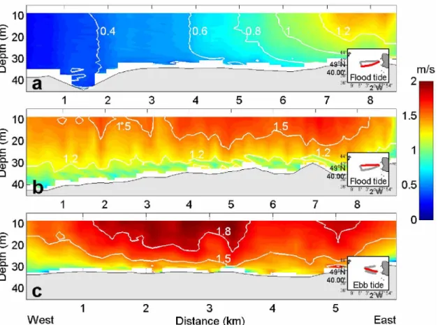
Underway velocity measurements allow assessing space-time variation of the tidal current. Velocity distribution on cross-sections during the towed ADCP surveys on flood and ebb tide are shown in Fig. 4. Tidal stream evolution on flood tide after the current reversal of LW is clearly seen on the southern cross- section, as the vessel was moving towards the shore (Fig. 4a). The velocity distribution with depth is nearly homogeneous for low current speed (<0.5 m/s). The velocity shear appears visible for higher speed
(~0.8 m/s) and becomes significant in tidal flow with speed > 1 m/s. The velocity shear increases as the current speed increases and the bottom boundary layer thickness attains 10-15 m (in a mean water depth of 30 m), roughly 50 minutes after the current reversal (to the right of 7 km tick mark in Fig. 4a).
The second cross-section shows the velocity distribution during the phase of fully developed flood flow (Fig. 4b). The largest velocities (~1.6-1.7 m/s) are found in the eastern part of the track, approximately 2 km offshore (along-track distance ~7 km), and the area occupied by high velocity tidal stream (u > 1.5 m/s) extends until 5-6 km offshore.
The towed ADCP survey reveals specific features of the tidal dynamics such as a more distant location of the tidal jet and its relatively stronger magnitude on ebb rather than on flood tide. During the ebb flow, the area of high-speed current is found at larger distance from the shore (Fig. 4c). The current velocity attains 2 m/s in a broad zone extending over 2 km.
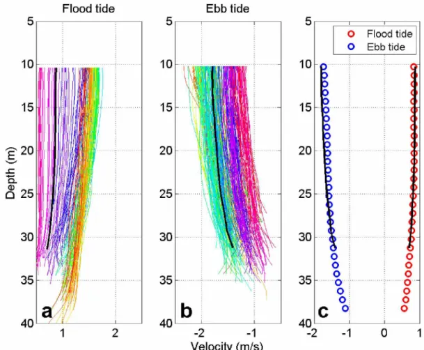
To further assess the velocity variation with depth, individual velocity profiles for flood and ebb flow were 1-minute averaged and smoothed by a low-pass filter (Fig. 5). Only profiles with depth averaged velocity exceeding 0.5 m/s were used in analysis. The colour transition from yellow to green accounts for tidal flow evolution. The largest velocity shear is found in the bottom 5-10 m thick layer for larger velocity values (> 1 m/s). For the time period of strongest current, an imbalance between flood and ebb flow can be inferred. A part of the difference in current speed is due to the neap to mean tide evolution that occurred during the day separating both surveys.
Underway ADCP observations were then compared to independent data - velocity measurements by a bottom-mounted ADCP. A fraction of the current record was selected when the towed ADCP was nearby the location of the bottom-mounted ADCP: the shortest distance was 10 m and the largest was ~450 m, on either side of the ADCP location. Velocity averaging was performed over 10-min interval for both instruments. Resulting velocity profiles are shown in Fig. 5c. A slightly better consistency was found for flood flow. We quantified the difference between each pair of profiles by calculating the mean relative error. The respective values of error are 6% and 15% for the flood and ebb tide velocities. This result is very encouraging as it shows the capability of a towed ADCP system to generate velocity profiles from underway measurements with relatively high accuracy levels. Ten minutes intervals seem to be appropriate for velocity averaging. However, it should be mentioned that the fraction of the cross-section covered by the towed ADCP measurements during a 10-min time interval has a length of ~1 km. Thus, similar comparison made in areas with large horizontal velocity gradients might provide worthwhile results.
In order to assess the model skill, the velocities recorded by towed ADCP along the track were vertically averaged and compared to the velocities derived from the model output. For all surveys, underway ADCP measurements started just after the current reversal. Therefore, velocities recorded during the first 30-60 minutes were very low and were not used in comparison. Only vertically averaged velocities recorded from 13:00 to 15:00 on flood tide (survey S3) and from 08:15 to 12:15 on ebb tide (survey S4) were compared with the model output at the mid-time of the respective periods. Vector maps of modeled velocities corresponding to that mid-time on flood and ebb tide are shown in Fig. 6. The first comparison is performed with the observed velocities varying in time and space. Visual inspection reveals a good agreement for the direction of the velocity vectors. During flood tide, the maximum discrepancy of the order of 0.1 m/s is found in the western part of the cross-section. Thus, the model velocity field on flood flow shows a general consistency with the observations for survey S3. On the contrary, during ebb tide survey (S4) which lasted four hours, significant differences in current speed are observed at different locations.
In order to take into account the tidal flow evolution during this survey period, the model-data misfit was estimated by performing space-time interpolation of model velocities into measurement points. The resulting discrepancy varied between 0.05 and 0.5 m/s (Fig. 7), with the maximum value achieved on ebb tide in the central part of the surveyed area where the strongest currents occur. In general, the model overestimates the velocity magnitude by 20% during ebb tide whereas, during flood tide, the discrepancy is two times lower (11%). Similar discrepancy is obtained for another flood tide survey, S1. Finally, a very close discrepancy level is obtained when comparing the average level of the kinetic energy within the study area (Tab. 1).
In order to evaluate how the velocity missing in the surface 10 m layer, after depth averaging, might account for the current speed over-estimation by the model, the profiles shown in Fig. 5c were extrapolated in the surface layer by using the power law (Lewis et al., 2017). The difference between the mean values of the extrapolated and initial velocities was found to vary from 0.01 to 0.04 m/s (1% to 2.5%) which is much smaller than model-data discrepancy (11% and 20%).
3.3 Space-time interpolation of underway velocity measurements
The ultimate goal of underway velocity measurements is to assess spatial variability of the velocity field in the area. However, the observed currents are affected by temporal evolution of the tide over the survey period. To account for this, the data has to be interpolated in both space and time. The resulting fields generated by OI, are a set of velocity snapshots generated on a regular space-time grid covering the entire period of observations. Fig. 8 shows an example of the interpolated velocity pattern at mid-times of the survey S3 and S4 (HW-1.30 hours and LW- 0.4 hours). The respective observations were projected to
the mid-time (also to all other time intervals) by the OI method using space-time corrélations of velocities provided by the model run for neap tide conditions.
The absolute difference in velocity magnitude e = |uOI - um| was estimated to quantify the overall agreement between the interpolated (uOI) and modeled (um) velocity fields at mid-time of each survey. The best agreement is obtained on flood tide where e is lower than 0.1 m/s in the majority of the domain with the exception of the northern part where e is ~ 0.5 m/s (Fig. 8, upper panel). Such a high difference might arise from large uncertainties in model bathymetry in this shallow region. The more significant effect of the OI is revealed during the second survey, on ebb tide, where e varies from 0.3 to 0.5 m/s revealing a large overestimation of current velocities by the model, especially in the central part of the domain (Fig. 8, lower panel).
The interpolating skill of the OI method was then assessed by performing a space-time interpolation of the model velocity onto measurement points. The optimally interpolated and modeled velocities were then compared (Fig. 7), and the overall quality of interpolation was quantified by estimating the mean relative difference with the data:
e =
1/2
(3)
Fig. 7a shows that during flood tide, observed, modeled and interpolated velocity curves fit well. The only exception occurs around the 50th minute after the beginning of the survey, when the observed velocities suddenly decreased. We attribute these disturbances in current measurements to the change of the towing direction at that particular time. The overall difference between observations and the model results is low, e = 0.11. After performing optimal interpolation, the difference decreases to 0.09 (Tab. 1). Thus, the model appears to be very effective in reconstructing the flood flow evolution.
Analysis of ebb flow velocities reveals higher levels of discrepancy. The largest misfit (up to 0.5 m/s) is found at three consecutive cross-sections (central times 8:15, 9:15, 9:45 in Fig. 7b). It matches a geographic location approximately in the centre of the study area (cf. Fig. 8 lower panel). The overall relative error during ebb tide is on the order of 0.2 (Tab. 1). Interpolation of velocity measurements provides a significant improvement of ebb flow field representation with a reduction of e down to 0.09 (i.e., by more than 50%).
The mean relative difference in current direction was also assessed and found to range between 5-7 degrees. This reveals a good capability of the model to simulate the current direction for the whole tidal cycle. OI does not provide any noticeable improvement in estimating the current direction.
In order to further assess the quality of interpolation and its ability to reproduce the time évolution of the flow field, the modeled and interpolated velocity time series were compared with velocities recorded by the bottom-mounted ADCP deployed within the survey area prior to underway velocity measurements. Fig. 9a shows that between the two surveying periods, the depth-averaged velocity gradually increases. The comparison demonstrates that during flood flow a good match between modeled and observed velocities is reached (Fig. 9b). The overall relative error em is within a range of 9% before OI of current measurements. The model tends to slightly overestimate the current speed at the beginning of the flood flow and underestimate the speed during the peak flow. The optimal interpolation reduces the difference to 5% (Table 1).
During the ebb flow, the absolute difference in current speed in the location of the bottom-mounted ADCP attains 0.5 m/s at peak flow (Fig. 9c). The relative error em for the whole ebb tide period is 18%. After performing the optimal interpolation, the overall agreement appears much better and the discrepancy eOI drops to 8% (Tab. 1). This result demonstrates the ability and efficiency of OI technique in reconstructing tidal motions in highly energetic coastal areas.
3.5 Power density distribution
The kinetic power density is commonly used for tidal stream energy quantification. It is defined as P = 0.5pu3, where p is the seawater density and u the current speed. The spatial distribution of the kinetic power density < P >, averaged over the selected period of flood (April 21, 13:00-15:00) and ebb flow (April 22, 08:15-12:15), was assessed by using modeled and optimally interpolated underway velocity measurements (brackets mean time averaging). The results are summarized in Fig. 10.
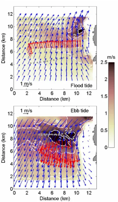
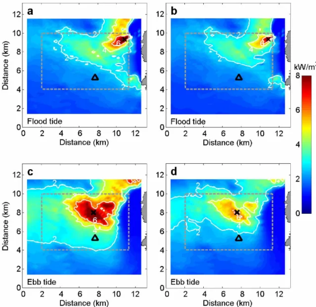
During flood flow, spatial distribution of the kinetic power density and location of the maximum of < P > appears similar for both modeled and optimally interpolated velocity fields. The largest power density is found approximately 2 km off the French coast in both cases (black crosses in Fig. 10a,b). During ebb flow, the strongest tidal stream migrated further offshore and the maximum power density is found at a distance of 5 km off the French coast. What is most important is the absolute difference in maximum power estimation revealed after interpolation. At both stages of the tidal cycle the maximum power density significantly decreases: from 11.5 to 8.5 kW/m2 for flood tide and from ~10 to 7 kW/m2 for ebb tide (26% and 33% respectively). The maximum value of power available in the flow is found larger at flood tide, but the overall level of power density and its spatial distribution, as shown in Fig. 10, appears larger at ebb tide (Fig. 10b,d). An explanation for this is not trivial. Alderney Race is a tidal channel with a complex bathymetry. Although ebb and flood phases have approximately equal duration, at flood tide, the strongest current is confined to the shore, South-North oriented, and aligned with it. At ebb tide, the tidal flow driven by topographic features propagates from the Northeast to the Southeast in a broader
stream, at a larger distance from the shore. This results in a different location of the maximum flow velocities and also in a different shape of power distribution, in particular, a broadening of large power density zone on the ebb tide.
To further quantify an overall change in tidal power resource as a result of optimal interpolation of underway velocity measurements, the power density was spatially averaged over the area covered by the measurements (gray dashed rectangles in Fig. 10) and in time: during two- and four-hour long periods of flood and ebb flow, when current velocities were larger than 1 m/s. The resulting estimates of power density P (the overbar stands for space-time averaging) were found significantly smaller after OI, compared to power density derived from model simulations. The respective values of power (POI) on ebb and flood tide became 1.7 and 2 kW/m2, showing smaller difference between tidal stages and a significant reduction (15% and 31%) compared to model derived values (Pm), estimated as 2 and 2.9 kW/m2 (Tab. 2).
The power density P was then estimated in one particular location where the velocity data was provided by independent measurements performed with bottom-mounted ADCP. The observed velocities were vertically and time averaged within flood and ebb tide periods corresponding to towed ADCP surveys. The results, presented in Tab. 2, show that all three power estimates are very similar on flood tide. Larger discrepancy is found on ebb tide, with the kinetic power density overestimated by the model by ~60%. Optimally interpolated velocities and independent point measurements provide very close estimates of the power density, POI and Pobs, with discrepancy less than 10% found on flood tide (Tab. 2).
4. Discussion
Tidal stream power is a promising solution for generating electricity from a highly predictable resource. An essential step towards market deployment of TEC arrays in highly energetic tidal channels, and in Alderney Race in particular, is an accurate assessment of spatial and temporal variability of tidal stream resource. Although numerous studies provided realistic assessment of the local hydrodynamics (e.g. Bahaj and Myers, 2004; Bailly du Bois et al., 2012; Thiébot et al., 2015; Coles et al., 2017; Guillou et al., 2018), none of them focused on identification of the key features of tidal dynamics at fine spatial scale, such as tidal current jet location, velocity shear, transient eddy dynamics, etc. Since Alderney Race is assumed to have the largest tidal stream potential in France, evaluating these metrics is essential to properly quantify the energy resource of the area. This is a key step in progressing towards commercial applications of energy conversion by the tidal stream turbines.
The studies mentioned above employed depth-averaged (2D) models. This is the most convenient, most practical, and less expensive approach for conducting tidal resource assessment during a long period. However, large spatial variations of velocity in fast-flowing environment, such as that of tidal energy sites,
are not easy to simulate with sufficient degree of details. Since the power output generated by a TEC is related to the cube of the current velocity, proper site screening is critical to the success of an installation. The main difficulty is to estimate the effect of micrositing, or the analysis of turbine placement, on the scale of two-four turbines’ size, (i.e. a hundred of meters). It is thus recommended to combine high- resolution modeling of the prospective site with accurate multipoint velocity measurements. However, in the case of large site dimension (e.g. ~10 x 10 km) and strong spatial variability of the tidal stream caused by topography variations, multipoint measurements might not correctly capture this variability.
In this sense, underway ADCP observations provide significant advantages over point measurements. The efficiency of underway velocity measurements for monitoring the tidal flow through the tidal channels was demonstrated in a number of recent studies (Gooch et al. 2009; Fairley et al., 2013; Evans et al., 2015). The transect time is a well-known limitation of vessel-based surveying compared to bottom-mounted current meters. To avoid distortion of the results caused by temporal variation of the tidal flow during the survey, very short (20-30 min) transects are repeatedly performed, usually around the peak tidal flow (e.g., Evans et al., 2015). This time limitation prevents continuous studies of larger domains which require surveying times comparable with the characteristic time scale of the velocity field (T ~ 2-4 hours).
This work presents a case study of two towed ADCP surveys performed over neap tide conditions in the French sector of Alderney Race. Low flow conditions were specially chosen for bottom-mounted ADCPs deployment and other fieldworks on site. Our study addresses the issue of comprehensive analysis of the velocity data to determine the space-time variations in the kinetic energy resource. The quality of assessment and the acquired results are improved by merging the data with the model output. The conventional approach of underway velocity profiling at tidal energy sites (e.g., Gooch et al., 2009; Fairley et al., 2013) was extended by using the optimal interpolation technique in both space and time to retrieve the entire evolution of tidal currents from the survey data. The technique, proposed by Sentchev and Yaremchuk (2016), employs tight space-time correlations in the tidal flow field that were accurately simulated by the high resolution model MARS-2D (Bailly du Bois et al., 2012). The use of space-time model covariances for synchronization of underway ADCP measurements is the major difference of the present technique compared to that employed by Goddijn-Murphy et al. (2013) for velocity interpolation in Pentland Firth. The OI method corrects the modeled output post-simulation but not the model control variables, such as boundary conditions, friction coefficient, bathymetry, etc. However, the ability of the method to adjust the model trajectory and the method’s simplicity largely compensate this limitation.
High resolution modeling used in our study was found to be very efficient in predicting the flow direction during both flood and ebb tide. However, comparison between model runs and observations demonstrated that, on average, the model overestimates the current speed by 11% during flood tide and by
20% during ebb tide. The latter discrepancy is quite large. How could the model results be improved? It is expected that the use of a finer grid (< 100 m) with corresponding bathymetry data could make the modeled velocities closer to the observations. However, such bathymetry data are not currently available. The use of spatially varying bed roughness could be another way to improve the modeled velocities. Many test simulations were performed using information on spatial variation in sediment size and, consequently, bed roughness. They did not show any improvement. To the best of our knowledge, no convincing results have been obtained in the English Channel to date. The homogeneous bed roughness (0.015 m) was found to provide the best result at local and regional scale. This value has been selected by comparing the model results with observed current velocities in many locations within the Channel Isles region (see Bailly du Bois et al., 2012 for more details). Another source of discrepancy is a limited capacity of the model to reproduce the non-linear effects of tidal wave propagation over highly irregular seabed. Even if the model is sought to be extensively validated, large model-data misfit was found in the north-eastern part of the domain where strong bathymetry gradients are found.
The OI technique proposed in this study is a valuable way to bypass the actual limits of numerical modeling. After performing OI, the level of velocity overestimation by the model drops down to 9% for both tidal phases. In contrast to pure model simulations, peak flow velocity was found larger on ebb tide. A migration of tidal current jet offshore was confirmed and the spatial extension of largest velocity area was assessed. This important feature of local tidal dynamics was demonstrated by towed ADCP velocity measurements for the first time. The capability of OI to identify significant inaccuracies in model simulations and to correct velocity fields in the error-prone regions is a notable advantage of the technique implemented in our study.
To further assess the efficiency of the OI method to correct the model results, we have performed comparisons with independent velocity measurements by bottom-mounted ADCP. It was demonstrated that the discrepancy between the static ADCP measurements (not used in OI) and optimally interpolated velocities decreased by a factor of two, compared to model prediction, for both flooding and ebbing tide stages. The model-data relative error drops down to 5% (on flood tide) and becomes comparable to the model validation error in two locations closest to the study area (c.f., section 2.4). The discrepancy appears slightly larger on ebb tide (8%) highlighting some difficulties of the model to simulate currents over highly irregular bathymetry. However, OI also shows some limitations. Its main weakness is that a significant improvement of modeling results can only be achieved for periods when observations are available. Outside the observation window, the model recovers its initial trajectory. A way to keep the model on a correct trajectory would be to provide the model with continuous measurements. In this sense, the static point ADCP measurements, currently used to assess the accuracy of interpolation, can extend the observation data set, even if the spatial impact of static point velocity measurements will be limited. High
Frequency (HF) radar measurements of surface currents represent another valuable source of data (c.f., Thiébaut and Sentchev, 2016, 2017).
Estimation of kinetic power density P was the subject of particular attention. The spatial distribution of power density, averaged over the selected periods of flood and ebb flow, < P >, was assessed by using modeled and optimally interpolated underway velocity measurements. Maximum values of < P > were found to be 11 kW/m2 and 10 kW/m2 on flood and ebb tide respectively. Spatial averaging of < P >, on the contrary, revealed larger values on ebb flow (~3 kW/m2) and the existence of large zones (on ebb and flood tide) with power density exceeding 4 kW/m2. The latter estimate, representative of neap tide conditions, is lower than the average values of P documented in other studies of Alderney Race.
To give an example, the highest value of 13.5 kW/m2 was found in the French sector of Alderney Race from the output of Telemac 2D model (Coles et al., 2017), while in the most recent modeling study, Guillou et al. (2018) evaluated the mean power density as 12.5 kW/m2, in the same sector. Large difference in power estimates, for neap tide conditions (in the present study) and averaged over longer period, highlights the need of experimental validation of modeling results for different tidal stages.
The kinetic power density derived from observations and model output (point by point comparison along the vessel circuit) showed that the velocity overestimation by the model leads to an overestimation of P by 16% and 65% on flood and ebb tide respectively. A spectacular reduction of these misfits (to 10% and 16% respectively) has been obtained by using OI technique. Space and time averaged power density estimates decreased by 15% and 31% respectively.
5. Conclusion
Underway ADCP measurements coupled with the 2D hydrodynamic model MARS post-simulation were used to assess the tidal circulation and tidal stream resource in Alderney Race - a highly energetic area where reliable, good quality measurements of tidal flow are scarce. Optimal interpolation was applied to process the velocity measurements from transect surveys at neap tide flood and ebb flow. The presented synthesis of the observed velocities with the model output provided a significant improvement in processing underway tidal velocity surveying both in terms of the reduction of model-data misfit and better consistency with independent (static point) velocity observations. As a consequence, a significant improvement in representation of the temporal and spatial variability of the tidal circulation was achieved. Constraining the model simulations by velocity measurements for evaluation of the kinetic power density demonstrated a noticeable reduction of the energy resource especially during ebbing tide, compared to pure model estimates.
We have fully met EMEC’s recommendations to carry out transect surveys by towed ADCP in order to assess the spatial variation in the velocity field over the site. The OI technique applied to the
surveyed data allowed us to go further in improving the quality of local resource assessment. We believe that merging high resolution velocity measurements and modeling makes the tidal stream potential estimation more accurate by reducing the uncertainties concerning the available resource at a tidal energy site. Thus, we strongly recommend standardizing the OI method for resource assessment at other sites.
Moreover, the remote sensing technique of velocity measurements (e.g., continuous data acquisition by land based HF radars) provides a new opportunity to improve the quality of local resource assessment by merging the massively incoming velocity data with the model outputs. The time scale of analysis can thus be significantly extended providing an annual estimate of the available resource. This is an interesting subject for future research.
Even if OI has demonstrated its ability to significantly improve the assessment of the temporal and spatial variability of the flow field, the use of depth-averaged velocities may lead to inaccurate estimation of the energy resource. A good overall agreement between (a) the 2D-model simulations constrained by velocity measurements and vertically averaged velocities observed by the bottom-mounted ADCP, and (b) velocity profiles obtained from both underway ADCP measurements and bottom-mounted ADCP, offers an interesting possibility of reconstructing the entire 3D evolution of the velocity field within the tidal cycle. For this purpose, the use of 3D version of the model is required.
By extending the interpolation algorithm to the MARS 3D model output, one could capture the variability of the velocity throughout the entire water column. The knowledge of the vertical variations of velocity is of first importance for tidal energy developers as large vertical gradients can generate turbulent fluctuations of velocity across a rotating tidal energy converter, causing unsteady load, and leading to a significant decrease of its lifespan. These negative effects could be increased by the combination of currents and significant waves. The 3D extension of the interpolation algorithm would require, however, consistent representation of the boundary layer physics and frictional effects by the model as well as the availability of an improved high-resolution bathymetry.
Acknowledgments
This work benefitted from the funding support from France Energies Marines and the French Government, operated by the National Research Agency under the Investments for the Future program: Reference ANR-10-IEED-0006-07. The study represents a contribution to the project HYD2M of the above program. We would like to acknowledge our colleague Max Yaremchuk from NRL for his help and valuable comments on the manuscript. We also acknowledge the skill of the scientific team, in particular, the head of the team, Louis Marié (Ifremer), the head of the research project, Anne-Claire Bennis (UNICAEN), the skipper and the crew of the R/V Thalia.
References
Assessment of tidal energy resource, Marine Renewable Energy Guides, EMEC, (http://www.emec. org. uk/standards), 2013.
Aviso-FES2012 was produced by Noveltis, Legos and CLS Space Oceanography Division and distributed by Aviso, with support from Cnes (http://www.aviso. altimetry.fr), 2012.
Bahaj, A. S., & Myers, L. (2004). Analytical estimates of the energy yield potential from the Alderney Race (Channel Islands) using marine current energy converters. Renewable Energy, 29, 1931-1945. Bailly du Bois, P. B., Dumas, F., Solier, L., & Voiseux, C. (2012). In-situ database toolbox for short-term
dispersion model validation in macro-tidal seas, application for 2D-model. Continental Shelf Research, 36, 63-82.
Bailly du Bois, P. B., Pouderoux, B., & Dumas, F. (2014). System for high-frequency simultaneous water sampling at several depths during sailing. Ocean Engineering, 91, 281-289.
Bretherton, F. P., Davis, R. E., &Fandry, C. B. (1976). A technique for objective analysis and design of oceanographic experiments applied to MODE-73. Deep Sea Research, 23, No. 7, pp. 559-582.
Bryden, I. G., & Couch, S. J. (2006). ME1—marine energy extraction: tidal resource analysis. Renewable Energy, 31(2), 133-139.
Coles, D. S., Blunden, L. S., &Bahaj, A. S. (2017).Assessment of the energy extraction potential at tidal sites around the Channel Islands. Energy, 124, 171-186.
Draper, S., Adcock, T. A., Borthwick, A. G., & Houlsby, G. T. (2014). Estimate of the tidal stream power resource of the Pentland Firth. Renewable Energy, 63, 650-657.
Evans, P., Mason-Jones, A., Wilson, C. A. M. E., Wooldridge, C., O'Doherty, T., & O'Doherty, D. (2015). Constraints on extractable power from energetic tidal straits. Renewable Energy, 81, 707-722.
Fairley, I., Evans, P., Wooldridge, C., Willis, M., & Masters, I. (2013). Evaluation of tidal stream resource in a potential array area via direct measurements. Renewable Energy, 57, 70-78.
Gandin, L. (1963). Objective analysis of meteorological fields, Gidro-meteorologichoskoeIsdatel'stvo, Leningrad, translated from Russian, Israel Program for Scientific Translation, Jerusalem. QJR Meteorol. Soc, 92, 447.
Geyer, W. R., & Signell, R. (1990). Measurements of tidal flow around a headland with a shipboard acoustic Doppler current profiler. Journal of Geophysical Research: Oceans, 95(C3), 3189-3197. Goddijn-Murphy, L., Woolf, D. K., & Easton, M. C. (2013).Current patterns in the Inner Sound (Pentland
Firth) from underway ADCP dataJournal of Atmospheric and Oceanic Technology, 30(1), 96-111. Gooch, S., Thomson, J., Polagye, B., & Meggitt, D. (2009). Site characterization for tidal power. In
OCEANS 2009, MTS/IEEE Biloxi-Marine Technology for Our Future: Global and Local Challenges (pp. 1-10). IEEE.
Guillou, N., Neill, S. P., & Robins, P. E. (2018). Characterising the tidal stream power resource around France using a high-resolution harmonic database. Renewable Energy, 123, 706-718.
Karsten, R. H., McMillan, J. M., Lickley, M. J., & Haynes, R. D. (2008). Assessment of tidal current energy in the Minas Passage, Bay of Fundy. Proceedings of the Institution of Mechanical Engineers, Part A: Journal of Power and Energy, 222(5), 493-507.
Lazure, P., & Dumas, F. (2008). An external-internal mode coupling for a 3D hydrodynamical model for applications at regional scale (MARS). Advances in water resources, 31(2), 233-250.
Legrand, C. (2009). Assessment of tidal energy resource: Marine renewable energy guides. European Marine Energy Centre.
Lewis, M., Neill, S. P., Robins, P. E., & Hashemi, M. R. (2015). Resource assessment for future générations of tidal-stream energy arrays. Energy, 83, 403-415.
Lewis, M., Neill, S. P., Robins, P., Hashemi, M. R., & Ward, S. (2017). Characteristics of the velocity profile at tidal-stream energy sites. Renewable Energy, 114, 258-272.
MacMahan, J., Vennell, R., Beatson, R., Brown, J., & Reniers, A. (2012). Divergence-free spatial velocity flow field interpolator for improving measurements from ADCP-equipped small unmanned underwater vehicles. Journal of Atmospheric and Oceanic Technology, 29(3), 478-484.
Myers, L., & Bahaj, A. S. (2005). Simulated electrical power potential harnessed by marine current turbine arrays in the Alderney Race. Renewable energy, 30(11), 1713-1731.
Plus M., Dumas F., Stanisière J.-Y., Maurer D., (2009). Hydrodynamic characterization of the Arcachon Bay, using model-derived descriptors. Continental Shelf Research, 29, 1008-1013.
Polagye, B., & Thomson, J. (2013). Tidal energy resource characterization: methodology and field study in Admiralty Inlet, Puget Sound, WA (USA). Proceedings of the Institution of Mechanical Engineers, Part A: Journal of Power and Energy, 227(3), 352-367.
Sentchev, A., &Yaremchuk, M. (2016).Monitoring tidal currents with a towed ADCP system. Ocean Dynamics, 66(1), 119-132.
Simpson, J. H., Mitchelson-Jacob, E. G., & Hill, A. E. (1990). Flow structure in a channel from an acoustic Doppler current profiler. Continental Shelf Research, 10(6), 589-603.
Thiébaut, M., & Sentchev, A. (2016). Tidal stream resource assessment in the Dover Strait (eastern English Channel). International Journal of Marine Energy, 16, 262-278.
Thiébaut, M., & Sentchev, A. (2017). Asymmetry of tidal currents off the W. Brittany coast and assessment of tidal energy resource around the Ushant Island. Renewable energy, 105, 735-747. Thiébaux, H., & Pedder, M. (1987).Spatial objective analysis with applications in atmospheric science.
London: Academics Press.
Thiébot, J., du Bois, P. B., & Guillou, S. (2015). Numerical modeling of the effect of tidal stream turbines on the hydrodynamics and the sediment transport-Application to the Alderney Race (Raz Blanchard), France. Renewable Energy, 75, 356-365.
Vennell, R. (1994). Acoustic Doppler current profiler measurements of tidal phase and amplitude in Cook Strait, New Zealand.Continental Shelf Research, 14(4), 353-364.
Vennell, R. (2006). ADCP measurements of momentum balance and dynamic topography in a constricted tidal channel.Journal of Physical Oceanography, 36(2), 177-188.
Vennell, R., & Beatson, R. (2009). A divergence-free spatial interpolator for large sparse velocity data sets. Journal of Geophysical Research: Oceans, 114(C10).
Venugopal, V., Davey, T., Smith, H., Smith, G., Holmes, B., Barrett, S., ...& Lawrence, J. (2011). EquiMar.Deliverable D2. 2. Wave and tidal resource characterisation.
Walters, R. A., Tarbotton, M. R., & Hiles, C. E. (2013). Estimation of tidal power potential. Renewable Energy, 51, 255-262.
Tables
Table. 1. Number of the observation points (N), the mean kinetic energy per unit volume diagnosed from two ADCP surveys (KEobs), from the respective model runs (KEm), the misfit between the observed and modeled (em), and observed and optimally interpolated current speed (eOI) in observation points. The misfit in two right columns is estimated by comparing the depth-averaged velocity provided by the bottom-mounted ADCP with model velocity (em,) and optimally interpolated velocity (eOI).
Towed ADCP
Bottom-mounted ADCP
Survey N KEobs
(J/m3) (J/m3)KEm em eOI em eOI Apr. 21, 12:30-15:00 UTC Flood tide 240 780 800 0.11 0.09 0.09 0.05 Apr. 22, 07:00-12:15 UTC Ebb tide 320 1050 1400 0.2 0.09 0.18 0.08
Table. 2. Max(< P >): maximum value of the kinetic power density (in kW/m2) time averaged over the surveyed period on flood and ebb tide. P: power density time averaged and space averaged over the area covered by underway velocity measurements. P: time averaged kinetic power density derived from the bottom-mounted ADCP observations (Pobs), from the model (Pm), and after performing OI of velocities (POI) in a grid point closest to ADCP location.
Kinetic power density
Survey Max(<Pm>) Max(<POI>) Pm Po\ Pm Poi Pobs
Apr. 21, 13:00-15:00 UTC Flood tide 11.5 8.5 2 1.7 0.9 0.8 0.8 Apr. 22, 08:15-12:15 UTC Ebb tide 10.3 6.9 2.9 2 1.9 1.3 1.2
Figure captions
Fig. 1. Left panel: Map of the central part of the English Channel and location of Aldemey Race (red rectangle). Black dashed rectangle shows the domain used for high-re solution modeling. Right panel: Study area (gray dashed rectangle) located between the west coast of Cotentin (France) and Alderney Island (U.K.) with bathymetry (m) given in gray, and four towed ADCP surveys in April 2017. Surveys on April 21 12:30-15:00 UTC (green) and on April 22 07:00-12:15 UTC (blue) are used for detailed analysis. Brown dot and dashed lines show the tracks of two other surveys reported in this work: on April 20 12:10-14:10 UTC and on April 21 09:00-11:00 UTC. Red triangle denotes the location of the bottom-mounted ADCP.
Fig. 2. Upper panel: Time series of the model-derived SSH in Goury harbour (black) and velocity magnitude (blue) in a point located in the middle of the domain. Light and dark gray shading shows the periods of four towed ADCP surveys referred to as S1-S4.
Lower panel: Time series of the model-derived velocity in the same middle point of the domain. Red dashed lines match the neap tide period used for estimation of model covariances. Dark gray shading shows two surveyed periods used for the detailed analysis (S3: on April 21 12:30-15:00 UTC and S4 on April 22 07:00-12:15 UTC). Light gray shading shows model ensemble members of the survey S3.
Fig. 3. The experimental platform Dynalest carrying a 600 kHz RDI ADCP and towed by the R/V Thalia in Alderney Race.
Fig. 4. Current speed (1-min averaged) along the cross-sections on flood tide (a,b) and ebb tide (c). The cross-section location is given in red in the insert.
Fig. 5. Current velocity profiles (1-minute averaged) derived from towed ADCP measurements during flood tide (a) and ebb tide (b) surveys. Only profiles with the vertically averaged velocity magnitude exceeding 0.5 m/s are shown. Color scale accounts for current velocity evolution from 0.5 m/s (brown) to maximum values (light green). 10-min averaged profiles corresponding to the period when the towed ADCP was nearby the bottom-mounted ADCP are given in black for flood and ebb tide surveys respectively. (c) Velocity profiles derived from the bottom-mounted ADCP (circles) and towed ADCP (black lines) for exactly the same 10-minute intervals and nearby locations. The location of the bottom- mounted ADCP is given in Fig. 1.
Fig. 6. Vertically averaged underway velocities (red vectors) obtained during the survey on April 21, 13:00-15:00 (upper panel) and on April 22, 08:15 to 12:15 (lower panel). Modeled velocity vectors (blue) and velocity magnitude (background shading) were taken at mid-time of each selected period: at HW- 1.30h (upper panel) and LW-0.4h (lower panel). Gray dots represent the measurement points with velocity less than 1 m/s.
Fig. 7. Tidal current velocities from the model (black), towed ADCP measurements (gray), and after Optimal Interpolation (red), projected onto measurement points, for the flood (a) and ebb tide (b). Observed velocities were depth-averaged.
Fig. 8. Optimally interpolated velocity field obtained at mid-time of the first (upper panel) and second (lower panel) survey: HW-1.30h and LW-0.4h respectively. Background shading shows the difference e between the modeled velocities and observed velocities interpolated at mid-time of each survey period. Gray points represent the location of the 1-min averaged towed ADCP measurements.
Fig. 9. Time series of depth-averaged velocity magnitude derived from the bottom-mounted (B-M) ADCP measurements (gray line and gray dots), model simulations (black), and underway velocity measurements optimally interpolated into a grid point closest to the ADCP location (red). Black dashed lines in the upper panel (a) show the periods of underway ADCP measurements presented in (b) and (c).
Fig. 10. Mean kinetic power density < P > derived from the model (a,c) and optimally interpolated velocities (b,d), averaged over flood and ebb tide periods: 21 Apr. 13:00-15:00 UTC (a,b) and Apr. 22, 08:15-12:15 UTC (c,d). Black crosses show the location of the maximum power density. Black triangle denotes the location of the bottom-mounted ADCP. Gray dashed rectangle shows the area covered by underway velocity measurements and used for spatial averaging of power estimates.
Figures Alderney Island France 20 2°W 40 Longitude (deg. W) 51 N England 21-Apr.-2017,12:30-15:00 UT C 22-Apr.-2017, 07:00-12:15 UT C rit**' 50 N Channe ■ Islands 1°W Distance (km)
Fig. 1. Left panel: Map of the central part of the English Channel and location of Aldemey Race (red rectangle). Black dashed rectangle shows the domain used for high-resolution modeling.
Right panel: Study area (gray dashed rectangle) located between the west coast of Cotentin (France) and Alderney Island (U.K.) with bathymetry (m) given in gray, and four towed ADCP surveys in April 2017. Surveys on April 21 12:30-15:00 UTC (green) and on April 22 07:00-12:15 UTC (blue) are used for detailed analysis. Brown dot and dashed lines show the tracks of two other surveys reported in this work: on April 20 12:10-14:10 UTC and on April 21 09:00-11:00 UTC. Red triangle denotes the location of the bottom-mounted ADCP.
Fig. 2. Upper panel: Time series of the model-derived SSH in Goury harbour (black) and velocity magnitude (blue) in a point located in the middle of the domain. Light and dark gray shading shows the periods of four towed ADCP surveys referred to as S1-S4.
Lower panel: Time series of the model-derived velocity in the same middle point of the domain. Red dashed lines match the neap tide period used for estimation of model covariances. Dark gray shading shows two surveyed periods used for the detailed analysis (S3: on April 21 12:30-15:00 UTC and S4 on April 22 07:00-12:15 UTC). Light gray shading shows model ensemble members of the survey S3.
Fig. 3. The experimental platform Dynalest carrying a 600 kHz RDI ADCP and towed by the R/V Thalia in Alderney Race.
Fig. 4. Current speed (1-min averaged) along the cross-sections on flood tide (a,b) and ebb tide (c). The cross-section location is given in red in the insert.
Fig. 5. Current velocity profiles (1-minute averaged) derived from towed ADCP measurements during flood tide (a) and ebb tide (b) surveys. Only profiles with the vertically averaged velocity magnitude exceeding 0.5 m/s are shown. Colour scale accounts for current velocity evolution from 0.5 m/s (brown) to maximum values (light green). 10-min averaged profiles corresponding to the period when the towed ADCP was nearby the bottom-mounted ADCP are given in black for flood and ebb tide surveys respectively. (c) Velocity profiles derived from the bottom-mounted ADCP (circles) and towed ADCP (black lines) for exactly the same 10-minute intervals and nearby locations. The location of the bottom- mounted ADCP is given in Fig. 1.
Fig. 6. Vertically averaged underway velocities (red vectors) obtained during the survey on April 21, 13:00-15:00 (upper panel) and on April 22, 08:15 to 12:15 (lower panel). Modeled velocity vectors (blue) and velocity magnitude (background shading) were taken at mid-time of each selected period: at HW- 1.30h (upper panel) and LW-0.4h (lower panel). Gray dots represent the measurement points with velocity less than 1 m/s.
Fig. 7. Tidal current velocities from the model (black), towed ADCP measurements (gray), and after Optimal Interpolation (red), projected onto measurement points, for the flood (a) and ebb tide (b). Observed velocities were depth-averaged.
Fig. 8. Optimally interpolated velocity field obtained at mid-time of the first (upper panel) and second (lower panel) survey: HW-1.30h and LW-0.4h respectively. Background shading shows the difference e between the modeled velocities and observed velocities interpolated at mid-time of each survey period. Gray points represent the location of the 1-min averaged towed ADCP measurements.
22/04 23/04 24/04 Day/Month, 2017 B-M ADCP — Model — Ol 1.5 0.5-Flood tide 12:30 13:30 14:30
Hours (UTC) on April 21,2017
B-M ADCP Model
Ebb tide
07 00 08:00 09:00 10:00 11:00 12:00
Hours (UTC) on April 22, 2017
Fig. 9. Time series of depth-averaged velocity magnitude derived from the bottom-mounted (B-M) ADCP measurements (gray line and gray dots), model simulations (black), and underway velocity measurements optimally interpolated into a grid point closest to the ADCP location (red). Black dashed lines in the upper panel (a) show the periods of underway ADCP measurements presented in (b) and (c).
Flood tide Distance (km) Ebb tide Distance (km) kW/m Flood tide Distance km Ebb tide Distance (km)
Fig. 10. Mean kinetic power density < P > derived from the model (a,c) and optimally interpolated velocities (b,d), averaged over flood and ebb tide periods: 21 Apr. 13:00-15:00 UTC (a,b) and Apr. 22, 08:15-12:15 UTC (c,d). Black crosses show the location of the maximum power density. Black triangle denotes the location of the bottom-mounted ADCP. Gray dashed rectangle shows the area covered by underway velocity measurements and used for spatial averaging of power estimates.