Continuous time algorithms for a variant of the dynamic traffic assignment problem

CONTINUOUS TIME ALGORITHMS

FOR A VARIANT OF THE

DYNAMIC TRAFFIC ASSIGNMENT PROBLEM

by

Jennifer M. Farver

B.S. Civil Engineering

University of California, Berkeley, 1998

Submitted to the Department of Civil and Environmental Engineering

in Partial Fulfillment of the Requirements for the Degree of

Master of Science in Transportation

at the

Massachusetts Institute of Technology

June 2001

@ 2001 Massachusetts Institute of Technology

All rights reserved

Signature of Author... ...

Department of Civil and Envi'o nmental Engineering

June 1, 2001

Certified

by.-Ismail Chabini

Assistant rofessor of Civil and Environmental Engineering

Thesis Supervisor

Accepted by -...

A

Oral Buyukozturk

Chairman,

MASSACHUSETTS INSTITUTE OF TECHNOLOGY

JUN

0 4 2001

on Graduate Studies

CONTINUOUS TIME ALGORITHMS FOR A VARIANT OF THE

DYNAMIC TRAFFIC ASSIGNMENT PROBLEM by

Jennifer M. Farver

Submitted to the Department of Civil and Environmental Engineering on June 1, 2001 in Partial Fulfillment of the Requirements for the Degree of

Master of Science in Transportation

ABSTRACT

The Dynamic Traffic Assignment (DTA) Problem is relevant to many transportation contexts, including planning and Intelligent Transportation Systems. Existing models have yielded approximate solutions to this problem using discrete-time methods. We present and implement several algorithms that enable exact continuous-time solution. The first of these algorithms is a practical continuous-time algorithm for a variant of the Dynamic Network Loading Problem (DNLP) in which input parameters take on a particular functional form. Specifically, path entrance flow rate functions are assumed to be stepwise and arc performance functions are assumed to be affine. These assumptions ensure that the resulting arc flow rate functions will be stepwise and enable computation of an exact solution. The second algorithm is an adaptation of the Bellman-Ford shortest paths algorithm to continuous-time, dynamic networks. We present algorithms for both the one-to-all and all-to-one variants of the dynamic shortest path problem. Both the DNLP and Dynamic Shortest Paths algorithms are implemented and tested on a sample

network.

Finally, we present a DTA solution algorithm which uses the DNLP and DSP algorithms to find a continuous-time solution. The DTA algorithm is also implemented and tested

on a sample network, thus a continuous-time DTA solution is found. Thesis Supervisor: Ismail Chabini

ACKNOWLEDGEMENTS

The author would like to thank Ismail Chabini for his guidance, insights and the patience he consistently showed throughout the preparation of this thesis. She would also like to thank her parents, Tom and Phyllis Farverffor their love and support and Ronak Bhatt for providing constant encouragement.

Contents

CHAPTER 1: INTRODUCTION... 11

1.1 T H E D T A P ROBLEM ... 12

1.2 MOTIVATION FOR A CONTINUOUS TIME DYNAMIC TRAFFIC ASSIGNMENT M O D E L ... 14

1.3 O BJECTIVES AND CONTRIBUTIONS... 15

1.4 B A C K G RO UN D ... 15

1.4.1 The D TA P roblem ... ... 16

1.4.2 The Dynamic Network Loading Problem ... 16

1.4.3 The Dynamic Shortest Paths Problem ... 17

1.5 T H ESIS O U TLIN E ... 18

CHAPTER 2: FORMULATION OF A CONTINUOUS-TIME DYNAMIC NETWORK LOADING MODEL ... 21

2.1 D ISCUSSION OF A SSUM PTIONS ... 21

2.2 N OTATION AND D EFINITIONS... 23

2.3 FORMULATION OF THE DYNAMIC NETWORK LOADING PROBLEM... 25

2.4 ANALYSIS OF THE DYNAMIC NETWORK LOADING PROBLEM ... 29

2.4.1 Properties of Inverse Functions... 30

2.4.2 Existence and Uniqueness of a Solution to the DNLP. Analysis of One Arc ... 3 2 2.4.3 Existence and Uniqueness of a Solution to the DNLP for General Networks ... 3 9 2.4.4 Solution Properties of the DNLP for a Class of Input Functions... 43 2.5 CONSTRUCTION OF A CONTINUOUS-TIME DYNAMIC NETWORK-LOADING

A LG O R IT H M ... 4 8

2.5.1 A DNLP Algorithm for a Single Arc ... 49

2.5.2 A DNLP Algorithmfor a Network ... 53

2.6 ALGORITHM IMPLEMENTATION... 57

2.6.1 Input Data Files and Representation of Paths... 58

2.6.2 Use of Vectors to Store Functions ... 59

2.6 3 Methodsfor Piecewise Functions ... 60

2.6.4 Storage and Computation of Functions ... 60

2.6 5 Other Notes on the Implementation ... 62

2.7 A LGORITHM T ESTING... 63

2.7.1 D N L P R esults... . 66

2.8 C ON CLU SIO N S ... 69

CHAPTER 3: CONTINUOUS TIME DYNAMIC TRAFFIC ASSIGNMENT ... 71

3.1 CONTINUOUS-TIME DYNAMIC SHORTEST PATHS . ... 73

3.1.1 Notation, Definitions and Assumptions...75

3.1.2 The One-to-All Minimum Travel Time Paths Problem: Formulation and Solution A lg orithm ... . . 76

3.1.3 The All-to-One Minimum Travel Time Pauhs Problem: Formulation and Solution A lg orithm ... . . 8 0 3.1.4 Implementation of a Dynamic Shortest Paths A lgorithm ... 83

3.2 A DTA SOLUTION ALGORITHM .. ... 86

3.2.1 The D TA A lgorithm ... 8 7 3.2.2 Some DTA Numerical Results... 88

3.3 C ON CLU SION S... 96

CHAPTER 4: CONCLUSIONS AND FURTHER DIRECTIONS OF RESEARCH ... 97

REFERENCES... 101

APPENDIX A -SAMPLE INPUT AND OUTPUT DATA FILES ... 103

N ETW O RK D A TA F ILE ... 103

A R C E x IT T IM E F ILE ... ... 105

APPENDIX B -METHODS FOR PIECEWISE FUNCTIONS... 107

INTEGRAL OF A STEPW ISE FUNCTION ... 107

VALUE OF THE INVERSE OF STRICTLY INCREASING PIECEWISE LINEAR FUNCTIONS.... 108

SUM OF Tw o STEPW ISE FUNCTIONS ... 109

M INIMUM OF Two PIECEWISE LINEAR FUNCTIONS ... 110

COMPOSITION OF INCREASING PIECEWISE LINEAR FUNCTIONS ... 112

APPENDIX C -SELECTION OF ARC PERFORMANCE FUNCTIONS...115

APPENDIX D -DNLP RESULTS... 119

CHAPTER

1

INTRODUCTION

The goal of Intelligent Transportation Systems (ITS) is to use technology to better exploit the physical capacity of existing transportation infrastructure. In particular, many of the technologies employed in ITS serve to collect, process, disseminate, and exploit information about the state of the transportation system. Information technology in ITS has many applications including commercial vehicle operations and non-predictive traveler information, however it is the ability to predict the future state of the transportation network that may provide the most significant advances in transportation efficiency. Predictive transportation models have applications for the transportation planner, the transportation service provider and the system user, providing tools for forecasting as well as for real-time route guidance.

Dynamic Traffic Assignment (DTA) models are predictive tools that, given O-D demands and network characteristics, determine demand on individual network components and the resulting cost of trips within the network. When coupled with demand models, DTA models provide predictive information that can answer various questions such as: "How congested will a given arc be in the future?" and "How long will

my commute be today? Should I take the usual route or an alternate route?" DTA models have many applications, but are particularly important in Advanced Traffic Management Systems in which they can be used to optimize the network via signals, changeable message signs, and other traffic control devices. In such applications, the goal is often to implement systems of real-time monitoring and control, which require DTA models and efficient solution algorithms. In this thesis we explore the properties and promise of a continuous-time DTA model and explore its advantages over discrete-time formulations.

1.1

The DTA Problem

Consider a network composed of arcs and nodes. A path is a set of successive arcs used to travel from some origin node to some destination node in our network. Each path or arc experiences some amount of flow as vehicles travel through the network from many origin nodes to many destination nodes. The DTA problem is to find time-dependent arc travel times, path travel times and arc flows, given a network with time-dependent origin-destination travel demands, a model of the relationship between arc flows and arc travel times and some assumptions regarding user route choice.

The DTA problem can be formulated by either simulation or analytical methods. While simulation has been used extensively to date to obtain DTA solutions, analytical models present several distinct advantages. Firstly, they require only one "run" to obtain a solution and there is no variability in the solution obtained. Secondly, analytical models can be constructed such that they possess theoretical attributes that permit the development of efficient solution algorithms. For these reasons, in this thesis we present an analytical formulation of the DTA problem.

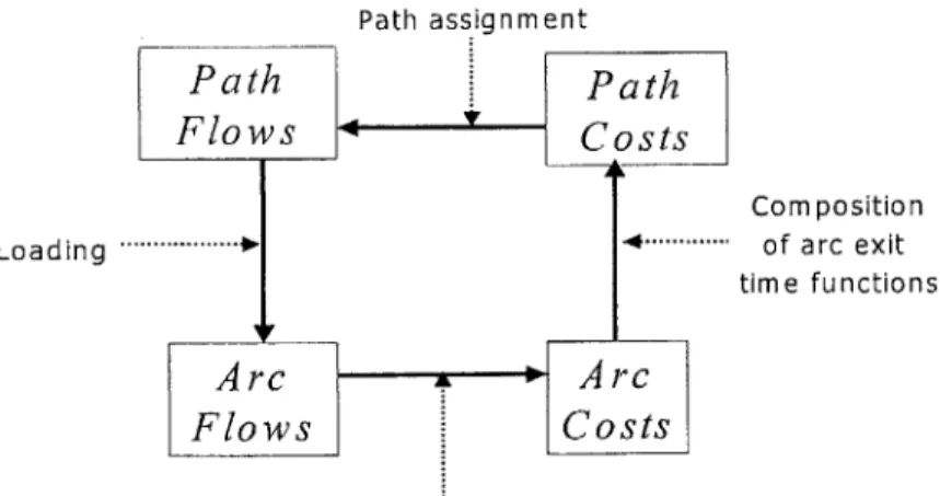
Figure 1 shows a simple DTA framework. Given a set of time-dependent path flows on a network, we calculate flows on the component arcs. From these arc flows, we can determine the total flow on a given arc at any time in the analysis period. Travel time on

an arc is dependent on these total flows, as described by arc performance functions. By composing the exit time functions of arcs along a path, we can then calculate the time-dependent travel time on each path. We then use a shortest path algorithm to determine minimum time paths between each O-D pair and assign O-D demands to these paths to obtain a set of path flows. These flows are then averaged with those of previous iterations. DTA algorithms seek to find a set of path flows such that traversing the DTA loop no longer yields a significant change in the values of the variables.

The DTA problem is composed of several sub-problems for which specialized algorithms are developed. To calculate path costs from arc costs, we use a dynamic variant of a standard shortest path algorithm. Calculating arc travel times from path flow rates is a sub-problem referred to as the Dynamic Network Loading Problem (DNLP) for which DNLP algorithms are developed. In this thesis we present a continuous-time DNLP model and a corresponding continuous-time Dynamic Shortest Paths (DSP) solution algorithm. For each, we first present the theoretical background of the problem before presenting the algorithm itself. We then present a DTA algorithm which uses the above

algorithms as subroutines to find a continuous-time DTA solution.

Path assignment

Path Path

Flows * Costs

Composition Loading ...'" 0. ... ' of arc exit

time functions

Arc A Arc

Flows Costs

Arc Performance

Figure 1: Components of a DTA Model

1.2

Motivation for a Continuous Time Dynamic Traffic

Assignment Model

Previous, discrete-time DTA models approximate the behavior of a network, much as numerical integration methods approximate the properties of a function. Time is discretized in small intervals and we make approximations at each interval. Like numerical integration methods, the efficiency of discrete-time models can be improved by decreasing the width of the interval; this is desired particularly in regions of sharp change. From a computational standpoint, the compromise made by increasing accuracy is one of efficiency since a greater number of iterations results in a greater run time. More sophisticated approaches may attempt to balance efficiency and accuracy by performing more computations in regions of rapid change and fewer in less dynamic regions. The success of these approaches however, is limited by the amount of a priori knowledge about the network's dynamics.

Continuous-time methods may have two primary advantages over their discrete-time analogs. First, given functional forms that allow us to obtain exact integrals on a computer, continuous-time algorithms may yield exact solutions. Instead of approximating network behavior over an interval by calculating parameters at many intermediate points, a continuous-time algorithm can describe network behavior in functional form. Thus, values of network parameters may be known exactly for all times contained in the interval of interest.

While the continuous-time approach yields algorithms with the advantage of being the most accurate available, it also provides a tool for benchmarking approximate algorithms. Various algorithms can then be compared not only based on run time, but on their error as compared to an exact, continuous-time solution.

A second advantage of continuous-time algorithms is that they are efficient in the sense that they may perform exactly the number of computations required to obtain a solution.

Values of network variables need only be determined at certain time instants; doing so allows us to completely specify the their values at all times in the analysis period. Thus, network behavior is completely and exactly specified by performing the minimum number of computations and a continuous-time model may prove more successful at responding to a network's dynamics than a discrete-time model. This may have implications for the algorithm's efficiency as well as for its data storage requirements, particularly for networks in which certain time intervals or arcs are much more dynamic

than others.

1.3 Objectives and Contributions

The objectives of this thesis are to:

. develop an exact, continuous time algorithm for the Dynamic Network Loading Problem, assuming stepwise path flow rate functions, affine arc performance functions and a deterministic, user-optimum users' behavior model;

. illustrate the concepts of the continuous-time Dynamic Shortest Paths problem and provide a simple algorithm for its solution;

. present a Dynamic Traffic Assignment algorithm that uses the above DNLP and DSP algorithms as subroutines to obtain an exact, continuous-time DTA solution; and

. implement these algorithms and test them on a small network in order to verify their correctness and illustrate properties of their solutions.

1.4

Background

In the following section we provide a brief summary of the developments in the literature that are pertinent to our problem. This includes work on discrete-time variants of the component algorithms as well as any existing continuous-time methods.

1.4.1 The DTA Problem

Existing work on the DTA problem is based on the DTA framework shown in Figure 1. Algorithms are developed for the Dynamic Network Loading Problem and the Dynamic Shortest Paths problem and a users' behavior model is adopted to reflect how flow is allocated among paths, once path travel times are known. In a simple users' behavior model, all users may choose the path of minimum travel time from their origin to their destination, while a more complex model may take into account the user's perceptions of travel time and route choice preferences. Inputs to the problem are O-D flow rates and the arc performance functions that model arc travel time as a function of the total flow on an arc.

Existing DTA algorithms have discretized time, calculating network variables for each time interval in the analysis period. Thus, discrete-time Dynamic Network Loading and Dynamic Shortest Paths algorithms exist in the literature. For the continuous-time problem, continuous-time Dynamic Shortest Paths algorithms have been developed, however no practical continuous-time Dynamic Network Lading algorithms exist, to date. In order to generate a continuous-time DTA solution, it is necessary to develop a continuous-time Dynamic Network Loading algorithm and ensure that DTA loop can be traversed using continuous-time variables. The reader is referred to Chabini and He (2000) and Chabini and Kachani (1999) for an overview of analytical DTA models.

1.4.2 The Dynamic Network Loading Problem

The Dynamic Network Loading Problem is to determine arc travel times, given a network with are performance functions and time-dependent path flows. Previous work on the Dynamic Network Loading problem has focused both on its mathematical solution properties and on the development of solution algorithms.

In Chabini and Kachani (1999), various properties of the DNLP were established for the class of problems in which arc performance functions are continuously differentiable and path flow rates are Lebesgue Integrable. The results are generalized for models that are linear or non-linear. The proven properties are:

1. the strong FIFO property is verified (the FIFO property will be discussed in Chapter 2),

2. the exit flow rate function is Lebesgue Integrable, nonnegative and bounded from above, and

3. the DNLP possesses a solution and this solution is unique.

The reader is referred to Chabini and Kachani (1999) for details of the proofs including the bounds on various function values.

Existing algorithms for the Dynamic Network Loading problem are of two types: those that iterate over network components and those that move chronologically. The first type, called I-Load, operate in a fixed-point manner, searching for a solution that verifies the constraints, using the Method of Successive Averages as a solution approach. The

second, C-Load, move forward in time, calculating arc parameters as flow is propagated

through the network. Discretized time intervals are used in these computation-s. Computational results of these two algorithms have been found to be similar (Chabini and He 2000), however because neither convergence nor uniqueness of solution for I-Load can be proven, C-I-Load has been recommended as the preferable network-loading algorithm.

1.4.3 The Dynamic Shortest Paths Problem

The Dynamic Shortest Paths problem is to determine the time-dependent shortest paths in a network, given its time-dependent arc travel times. Like the static shortest paths problem, the dynamic problem has several variants including one-to-all nodes and all-to-one node. Furthermore, in this dynamic problem we may define the problem in terms of

either the departure times of flows, or in terms of their arrival times. The Dynamic Shortest Path problem can also be posed for FIFO or non-FIFO networks, however the networks that verify the FIFO property are of interest in this thesis.

Existing algorithms for the discrete-time Dynamic Shortest Paths problem include dynamic extensions of well-known static shortest paths algorithms including the label-correcting algorithm and the Bellman-Ford algorithm. Additional algorithms, such as Algorithm DOT (Chabini 1997, 1998) have been developed specifically for the dynamic problem. Testing of these algorithms has shown that Algorithm DOT is faster. The Bellman-Ford algorithm also performed well as compared to label-correcting.

For the continuous-time variant of the dynamic shortest paths problem, the label-correcting algorithm and Algorithm DOT have been implemented. In this thesis, we consider a continuous-time adaptation of the Bellman-Ford algorithm. The reader is referred to Dean (1999) for a more exhaustive treatment of the dynamic shortest paths problem, with particular attention given to the continuous-time variant.

1.5 Thesis Outline

The goal of this thesis is to formulate and implement a continuous-time DTA solution algorithm. To do so, we will also formulate and implement continuous-time DNLP and DSP algorithms. All of these developments will rely on networks whose parameters take on functional forms which permit exact continuous-time solutions. Arc performance functions are assumed to be affine; O-D flow rate functions are assumed to be stepwise and all users are assumed to travel along shortest paths.

Chapter 2 concerns the Dynamic Network Loading Problem. We present a variant of the problem in which arc performance functions are affine and path flow rate functions are stepwise. We discuss the advantages of this variant. Furthermore, we present theoretical properties of the problem including proofs of existence and uniqueness of a solution as

well as a proof that the resulting arc travel time functions are piecewise linear. Given these properties, we then present an algorithm for solving the DNLP in continuous time. Chapter 2 concludes with a discussion of the implementation and testing of the DNLP algorithn.

In Chapter 3 we illustrate how the DNLP algorithm can be used to obtain a continuous time solution to the DTA problem. We first discuss the continuous time Dynamic Shortest Paths problem, and formulate its optimality conditions for the one-to-all and all-to-one minimum travel time problems. We then present continuous time DSP algorithms and discuss the implementation of the one-to-all algorithm. Finally we present a DTA afgorithm which uses the above algorithms to find a continuous time DTA solution. This algorithm is also implemented and some numerical results are given.

In Chapter 4 we discuss the strengths and weaknesses of the algorithms developed in Chapters 2 and 3 and present some directions for further research.

CHAPTER

2

FORMULATION OF A CONTINUOUS-TIME DYNAMIC

NETWORK LOADING MODEL

In Chapter 1 we stated that the Dynamic Network Loading Problem is to determine arc travel times given a network with time-dependent path flows and a model of the relationship between flow and travel time on an arc. This statement of the problem is quite general and any of several models could be used to generate a solution. Having recognized the limitations of discrete-time models, we now seek to develop a model of the DNLP that can be solved in continuous time. To do so, we first make some simplifying assumptions and discuss their validity. We then present a mathematical formulation of the model which defines network parameters and expresses their relationships to one another. We derive various theoretical properties of the model which enable the development of an exact, continuous-time DNLP algorithm. These properties include existence and uniqueness of a solution, as well as functional properties of the unknown variables. Finally, we develop a continuous-time DNLP algorithm and discuss

its implementation and testing on a sample network.

2.1 Discussion of Assumptions

In order to develop an exact, continuous-time DNLP algorithm, we make two major simplifying assumptions. First, we assume path flow rate functions to be stepwise. Second, we assume the relationship between an arc's total flow and its travel time (called an arc performance function) to be affine.

Before constructing an algorithm, we consider the strengths and weaknesses of these simplifying assumptions. We first consider the assumption that path flow rate functions are stepwise functions. When selecting inputs to our model, it is likely that we would wish to work from some real world data set to determine origin-destination demands. Recognizing that:it is likely that such a data set would be represented as a set of discrete data points, it is advantageous to work with the continuous-time function that naturally follows from discretized data - a stepwise function. Furthermore, it should be recognized that stepwise functions have the additional benefit of easily approximating the shape of any function. Thus, we consider the assumption that path entrance flow rate functions are stepwise to be both realistic and flexible.

With regard to the assumption that arc performance functions are affine, we consider the degree to which the arc performance model represents the real world. Consider the travel time on an arc. In the real world, we know that if the flow on the arc is small enough, a vehicle may traverse the arc without experiencing congestion-related delay. In this case, the vehicle experiences the arc's free flow travel time, . Suppose, however that a

vehicle enters a congested arc. We may wish to model the congestion as a queue that the vehicle must join before exiting the arc. The vehicle's travel time r , is then equal to 1-., plus the time spent in queue. For a queue with a deterministic service rate C and X,

enqueued vehicles, we may express this as:

I = Xq IC +r #.

We note that this is equation is an affine function, but that it depends on X,,,, not on the

total flow on the arc, X. In our model, we wish the arc's travel time to be an affine function of X:

If we assume 02 = r, then we note that any amount of flow X, no matter how small, results in a travel time greater than . This is a weakness of the model, because in real world networks, positive flow rates can indeed experience free flow travel conditions. Furthermore, the assumption that congestion can be adequately represented by a single linear term is overly simplistic. Nevertheless, an affine function is perhaps the most simple way to model the relationship between flow and travel time and possesses theoretical properties which enable an "elegant" solution to the DNLP. In Section 2.4 we will show that by using the linear model above, combined with stepwise path flow rate functions results we can ensure that other network variables maintain functional forms that enable continuous.time solution. It is this latter advantage of the linear model that provides the most compelling argument for its use.

Another advantage of this model is its adaptability to future extensions. We recognize that a natural extension of this model is to use piecewise linear arc performance functions to more accurately model the relationship between flow and travel time. This topic is left to further research.

2.2

Notation and Definitions

In order to represent a physical traffic network in a mathematical model we construct a conceptual network, G = (N, A) in which N is the set of nodes and A is the set of arcs.

The network consists of a set of paths P, each of which has an origin r and a destination s. We denote by K, the set of paths connecting r and s. We also denote by K, the set

of paths passing through arc a. For some arc a on path p, we denote by 5 the previous arc on p and by i the next arc on p .

Below we present a list of variables used throughout this chapter. Some of the variables express flow rates on each path - we call these path variables; similarly arc variables express flows, flow rates and travel times on each arc. Additionally, we use arc-path

variables to express flows and flow rates on a given arc and path. Finally, we present time variables, which specify the time interval of interest.

Path Variables

ft I(t) departure flow rate on path p for O-D pair (r,s) at time t;

Arc Variables

U', (t) cumulative flow that has entered arc a during interval [0, t];

V, (t) : cumulative flow that has exited arc a during interval [0,t]

X'1 (t) total flow on arc a at time i;

D, (X, (t)): travel time function of arc a, where X,, (t) is amount of flow on arc a;

A, minimum value of D, (X,,(t)) over all times t in the interval [0,t]. If

D,(.) is strictly increasing, then A, equals the free flow travel time,

Di(0);

A : min(k,);

S, (t) : exit time of flow entering arc a at time t. s,, (t) = t + D

Arc-Path Flow Variables

(a, p) an arc-path pair;

(r, s) the origin-destination pair of path p;

u', (t) entrance flow rate at time t for arc a and path p;

v', (t) exit flow rate at time t for arc a and path p;

U:;;A (t) cumulative entrance flow at time t for arc a and path p;

Va' (t) cumulative exit flow at time t for arc a and path p;

X', (t): total flow on arc a due to path p at time t. The total number of vehicles on

an arc at time t is then X,(t)= X, (t);

p7EK,.

Time Variables

t index for continuous time;

[0, T] O-D traffic demand period; and

[0, T.I: analysis period. T is the lease instant, greater than T after which no flow remains in the network.

FIFO Property

To conclude this section, we present a definition of the First In First Out (FIFO) property which will be referred to in subsequent sections. In this thesis, we consider an arc to verify the FIFO property if:

s (t,)< sl(t2) _Vti < t?

In the literature this is referred to as the strict FIFO property (Chabini and Kachani (1999)). Other definitions of the FIFO property exist, the weakest of which is:

s,(t,) s s(t 2) Vt : t2 v, 1 t2 *

Alternately, one may refer to the strong FIFO property in which, for t, <t2, the

difference between s, (t,) and s, (t,) is at least some positive multiple of the difference

between t, and t, . The reader is referred to Chabini and Kachani (1999) for the details of these properties.

2.3

Formulation of the Dynamic Network Loading Problem

In the following section we state important relationships between the network variables that were presented in Section 2.2. These equations are the formulation of the dynamic

network loading model and describe arc dynamics, flow conservation, flow propagation, arc performance and initial/terminal conditions. Each of these equations is an accurate and general representation of how flows move through a transportation network; these equations are common to many dynamic network loading models. In a later section we will choose functions to approximate the relationship between flow and travel time on an arc. By choosing functional forms which ensure various solution properties, we can develop exact, continuous-time solution algorithms.

Arc Dynamics

The arc dynamics equations describe the alniount of flow on a given arc as a function of time. They state that the total flow on an arc depends on the arc's entrance and exit flow rates and that the difference between the arc's entrance and exit flow rates is equal to the rate of change of the total flow.

dX"(11 _{" (=U} ) V_{(t) - v" (t) V(r, s), Vp E K,, Va. (1)}

dt u

Flow Conservation

Flow conservation equations ensure that along a given path, no flow is lost or gained from one arc to the next on a given path--that is, for two successive arcs along a path, the amount of flow on the path exiting the first arc is equal to the amount of flow entering the second arc at any time t. For the first arc on any path, the entrance flow is equal to the known entrance flow of the path. These conditions are expressed mathematically as:

u[, (t)=

f,"()

for the first arc on any path and as:

up (t) = v" () V(r, s), Vp e K, (3 ) for all other arcs in which arc 5 follows arc a on path p.

Initial and Terminal Conditions

We impose initial conditions such that the network must be empty at time t = 0. They are:

U'(0)= 0, V(,'(0)= 0, X'(0) 0, V(r,s),Vp e K,,,, e p . (4)

The above initial conditions are assumed for ease of computation without loss of generality; any set of feasible initial conditions could be used. We likewise denote by

t = T, the time at which the network will again be empty.

U', (T, ) = V,'*"(T. , X,' (T. ) 0 , T. > 0 V(r, s), Vp c- K,,,a E= P

(5)

Equations (5) are the terminal conditions.

Arc Performance

Arc performance functions relate an arc's travel time to its total flow. Given our discussion of the advantages of a linear arc performance model, we use the equation:

D", (X,, ()) = 0,X( )+, V a e A ((61)

where O, and 0,,2 are the parameters of the arc performance function of arc a.

Flow Propagation

The following equations relate an arc's outflow to its inflow; they express flow conservation between an arc's origin and destination. In the literature, these equations are referred to as "flow propagation" equations. Though we feel that this terminology does not properly express the meaning of these equations, we retain it for consistency. At some time t, we know that all flows exiting the arc at time t must have entered the arc by time z such that z + D(, (z) t . If we denote by o a time at which an entering flow can exit the arc by time t, we can state that the cumulative exit flow on arc a for some path p with origin r and destination s is equal to the integral over all such times o. Mathematically, we have:

V(r, s), Vp e K,,, Va e p.

This flow propagation equation makes no assumptions about the overtaking behavior of vehicles on the arc. If we assume that the arc operates on a first-in first-out (FIFO) basis, we can state that flows exiting the arc at time t must have entered the arc at time s-' (t).

Furthermore, we know that the cumulative exit flow at time t is equal to the integral of the entrance flow over the interval [0,s-'(t)] (given the initial conditions). The flow propagation equation if FIFO is verified becomes:

xi,-' (i)

VJ/7j'(1) = ju2 "(co)dco) V(rs),Vp EK.,, _{Va e p .} (7)

SuU'

(t)

Summary of the Formulation

We now review the formulation of the model in terms of its known and unknown variables. By initial conditions, U, (0), V,'j7(0), and X' (0) are known values for all arcs, and paths. Ji (t) is also a known variable for all paths and times contained in the

analysis period. We also know the value of T. The unknown variables are:

a

To

0 U,,(t), V,(t), _{Xf,(t), D,(t), u,(t) and v,(t) Va, Vt e [O, T]}

The above summary lists the known and unknown variables of the dynamic network loading model. In Section 2.4 we rigorously prove that, given stepwise path flow rate functions and affine arc performance functions, a solution to this dynamic network loading models exists and this solution is unique.

tyu"'(co)dc 11/7;(t)=

2.4 Analysis of the Dynamic Network Loading Problem

The primary focus of the following section is to illustrate that, for a specific class of input functions, solution properties for the DNLP can be established which enable its solution in continuous time. More specifically, by assuming path flow rate functions to be stepwise and arc performance functions to be affine, we will prove that the other network variables take on piecewise forms. Arc and path flow rate functions are proven to be stepwise; cumulative arc and path flow functions and total flow functions are shown to be piecewise linear. Arc exit time functions are also proveh to be piecewise linear. In the algorithm, this knowledge of the functional forms will be exploited by calculating problem variables at function "breakpoints". Theorem I presents the functional forms of

the network variables that result from our choice of input functions.

In order to construct an algorithm to solve the DNLP as described in Section 2.3, we must first establish several mathematical properties of equations (1)-(7). In the following sections, we provide proofs of several lemmas regarding continuous, differentiable functions. These lemmas will assist us in proving the existence and uniqueness of.a solution to the DNLP, for single arc and later for a general network. Following the proof of existence of a solution, we prove that for the case of stepwise path flow rate functions and affine arc performance functions, the DNLP possesses a unique solution whose network variables take on a particular functional form. This knowledge leads to an "elegant" construction of a continuous-time dynamic network loading algorithm. Finally, we prove two theorems that assist us in specifying the length of time interval over which to iterate in our algorithm and establish a bound on the number of computations required to solve the DNLP. These theorems ensure that our DNLP algorithm will terminate after a finite number of iterations and provide a basis for discussion of the algorithm's theoretical run-time.

2.4.1 Properties of Inverse Functions

The following two lemmas establish properties of inverse functions. In constructing our algorithm in later sections, we will use s-'(t), the inverse of the function s,(t), thus the

following properties will prove useful. The proofs of Lemmas 1 and 2 are borrowed from Chabini and Kachani (1999), with some slight modifications for clarity.

Lemma 1 (Chabini and Kachani, 1999): Let g(-) be a continuously differentiable function on [0, T]. Iffor every x e [0, T] g'(x)# 0 , then g(.) is invertible on [0, T], its

inverse function g (-) is continuously differentiable on

[min(g(O),g(T)),max(g(O),g(T))] and, g' '(x) =

g (g (x))

Proof of Lemma 1 (Chabini and Kachani, 1999):

Since g(-) is a continuously differentiable function, g'(.) is continuous. Furthermore,

since for every x e [0, T], g'(x) # 0, we know that g'(.) has a constant sign. Hence, g(.) is either strictly increasing or strictly decreasing. Since every strictly monotonic

function is invertible, it follows that g(-) is invertible. Let g-'(.) denote the inverse

function of g(.). According to the definition of an inverse function, we have: g(g~'(x)) = x. If we differentiate both sides of this equation, we obtain:

-' '(x)g'(g '(x)) = 1. Rearranging terms, we have: gf''(x)= _ . According to

g' (g' (x))

the conditions of the lemma, g'(x) # 0 on [0, T], therefore g-''(x) is defined on

[g(0), g(T)] if g(-) is strictly increasing, or on [g(T), g(0)] if g(-) is strictly decreasing.

Equivalently, we can say that g-'(.) is continuously differentiable on

[min(g(0), g(T)), max(g(0), g(T))].

Lemma 2 (Chabini and Kachani, 1999): Let

f(-)

the interval [a, f -'(x)].

Proof of Lemma 2 (Chabini and Kachani, 1999):

Since

f(-)

f(.)

[f(a), f(b)].

We first prove that W. c [a,f-'(x)]. By assumption, for a given w e WA,, we have:

jf(w) x. Since w e [a, b] and

f(-)

f(a) f(w) x. Since

f

f~'(f(a))

f-'(f(w))

f'(x).

a 5 w <

f'

We now show that [a, h (x)] c W. For a given -w) e [a,

f~'(x)],

f'

Since

f(.)

f(ff

f(w)

Furthermore, since x c [f(a), f(b)] and f'(.) is increasing, it results that

f -(x) - [a, b]. Since w e [a,

f-'(x)],

[a, -~'(x)] c W, .

Since W. c [a, -'(x)] and [af~'(x)] c W,, we have proved that W, = [a, -~ (x)]. 0

2.4.2 Existence and Uniqueness of a Solution to the DNLP: Analysis of

One Arc

In order to prove the existence and uniqueness of a solution to the DNLP for a general network, we first prove the existence and uniqueness of a solution for a single arc. In addition to assisting us in understanding the proof for a general network, the results that we establish for the single arc will be used in the analysis of a general network.

This proof relies on several specific network properties, 'namely that arc performance functions are affine and entrance flow rate functions are stepwise. Proofs of similar results for a more general class of functions can be found in Chabini and Kachani (1999). For the model studied in this chapter the proof below is less complicated. At the'heart of the pioof is the fact that the solution verifies the FIFO property.

Theorem 1 For a single arc, if the pair (D, (-), f,,(.)) verifies the

following

(ii) the departure flow rate function f, (-) is stepwise, nonnegative and bounded from

above by some positive constant M then the following properties hold for the DNLP.

(i) the strong FIFO properly is verified; and

(ii) the DNLP possesses a solution and this solution is unique.

Proof of Theorem 1:

We present an induction proof of Theorem 1, which relies on establishing the existence and uniqueness of a solution, as well as the FIFO property for successive time intervals. The induction is over the indices of the time intervals, denoted by i. We define our time intervals such that for some interval [t, ,t1 ), ti,1 is the first time instant at which a flow

entering the arc at time t, may exit the arc. The sequences of instants t, is defined by

The following is the induction hypothesis for some time interval [t, , -).

Induction Hypothesis

For the interval [t,, t, ), the following properties hold:

(i) s,, (t) is piecewise linear and continuous over [t, ,tj ) and s', (t) > y, + a,,u, (t) where 0 < y, I ;

(ii) _{V,, (t) is piecewise differentiable over [t,,ti ) ;}

1

(iii) For every t e [ti,, ti), v,(t) and a,,

(iv) the DNLP has a solution on [0, t,1) and this solution is unique.

Before beginning the induction we establish several properties that hold for all times / in

the analysis period. Since we consider a single arc, we know u,(-)

f,(-).

U, (t) = fu(co)do.

Since u, (t) is unique and the integral operator is unique, we know U,() to be unique. Furthermore, because u, (-) is nonnegative, U, (-) is non-decreasing.

First Base Case: Time interval

_[0,t

)

dX₁

_,

dt

and by integration, we have

for U, (0)= 0, V, (0)= 0 and X,, (0)= 0. Additionally since no flow can exit before I,

V, (t) = 0, so X,, (t) = U,, (t) and

X,(t) = Ju(co)dwv.

Thus, like U,, () X, (-) is continuous and unique on [0, i,). We now consider s, (t) which is defined by:

s,(t) =t + D,(X,(t)).

Since X, (-) is continuous and unique and D,, (-) is affine, D,, (X, (t)) is continuous and

unique, and therefore s,, (t) is continuous and unique. We can also establish that b-ecause

t is strictly increasing, and X, (t) is non-decreasing, D, (X, (t)) is non-decreasing

and s, (t) is strictly increasing. Thus, on the interval

[0,

[0,

In later parts of this proof we will use the properties of s,, (t) to find an upper bound on the exit flow rate function. In particular, we wish to bound the slope of s, (t). We observe that:

s', (t)=I+D' X(t)) 'X =1+u t)'(X,,(1)).

di

Since D, (.) is affine, D', (-) is known to have a constant value, which we will denote by a,. Additionally, we replace the value ] with the variable yo to yield:

s' (t) =I + aju, (t).

We now construct a second base case. This base case differs from the first because we now examine an interval with positive exit flow. After constructing this second, "more general" base case, we complete the proof with an induction step. We again construct an interval such that vehicles entering at the beginning of the interval will not exit the arc before the end of the interval.

Second Base Case: Time interval [t,, t2

)-In the first base case, we proved that si, (t) is increasing on the interval [0, t). Since

si, (0) = t, and s, (t) = , then si, (t) is invertible. Using Lemma 1, we know sj (t) on

[t1,t2), s-'(t) e [0,t,) and (s-')'(t)= As sj (t) corresponds to the entry

s', (so ())

time for a flow which exits the link at time t, and s;'(t) e [0,t,), vehicles that exit arc a before a time t must have entered it before s-'(t) .

As Vi, (0)= 0, we then have:

V(t) = J (w)do Vt e

[t

Since u (-) is stepwise and unique on [0,t/i), V,(-) is piecewise linear and unique (ahd

therefore piecewise differentiable). Additionally, since u,(-) is nonnegative, V (-) must be non-decreasing. We can then compute v,(-) by differentiating V,(.). We obtain

v,(I)u= ((s) (s'(t)) , which must be nonnegative because u,,(-) is nonnegative

-~ 1

and s',, () is nonnegadve on the interval [0,t,). Given that (se)'(t)= we

s ,(s) (t))

obtain:

ul(s-(l)) V ,(t) =.

From the first base case, we know that u, (s-'(t)) is unique and si, (s-'(t)) is unique.

Si, '(s' (t)) must then also be unique because the derivative operator is unique. Thus,

v1(-) must also be unique. Furthermore, since s(si(t)) is strictly increasing, s', (s-'(t)) must be positive, thereby ensuring the positivity and existence of (-). Additionally, from the first base case we proved that:

s', (t) > yo + a,u,,(t) for t e [0, t,)

so we have:

Yo (t1))±au, (s 70 + atiU11(si't)

We also note that given the bound:

uf (setI (t))

ve,(t) <7 _a

0

(I+

aU,(s-'(t))

used in the proof of Theorem 1, we can obtain the bound:

We create this bound on v,, (), because as we shall see later in the proof, the exit time function s,, (t) depends on the difference between the entrance flow rate and the exit flow rate. By bounding the value of the exit flow rate, we can ensure that s, (t) is strictly increasing and thus that the FIFO property is preserved.

C

Since U, (-) and V, (-) are unique then X, (-) must also be unique according to:

X" W) = U"W)- V,(t ) .

Furthermore, since U,, (-) and V,, (-) are piecewise linear, then X,, (-) must be piecewise linear and D, (X,! (t)) must be piecewise linear and unique. Thus, s, (t) must also be piecewise linear. We have also shown that a solution to the DNLP exists on this interval and this solution is unique.

We now establish that s,(t) is strictly increasing on the interval . First, we recognize that

dX(t) dt = 1+ _{a,, (u,(t) - v, ())} Since v,(t) u (s"( , we have: 70 + a,,U,(SI (1)) r0 + a u, (s ' (t)) Sau, (t) + (I a~u(s t))

We recognize that the quantity u,, (t) is bounded from below by zero (because entrance flow rates are nonnegative) and from above by some positive constant M (because by assumption we do not permit flows of infinite flow rate), we have:

s ,'(t) a uY,()+ + o

Yo +aM

We know that a, and M are nonnegative, so we recognize that 0 < 0 < ;. 7o + alM

We denote by v, the quantity and we have:

70 +a,,M

sl,'(0) ! ;, + a,(0) .

We know that au,, u,, (t) and y are nonnegative, so sa'(t) must be nonnegative also.

Consequently, (strict) FIFO is verified on this interval.

To complete the proof, we now prove the existence and uniqueness of a solution, as well as the FIFO property for an interval

[tj+±

Induction Step: Time interval It,+, i)

In this interval we proceed in a manner similar to the second base case. By the inducdon hypothesis, we know that s (-) is piecewise differentiable and continuous over [t,,tie) and s',, (-) > 0 . We recall from Lemma 2 that s',, (-) must then be continuous over

[s,(t,),s, (t,+1)) = [ti, ti) as well as differentiable and unique.

We also have:

V,(t)= u(co)dco Vt e _{[t+ ,ti ),}

and since s-'(.) is differentiable and unique on

[t+,t+),

unique, V, (-) must also be differentiable and unique. We can then obtain

v,(t)'= ((s)'(t)) -u,(s- (t)), and:

s')

as we did in the second base case. We note that U,(-), V, (-) and X,, (-) are unique and piecewise linear. Thus, a solution to the DNLP exists and this solution is unique.

From the induction hypothesis, on interval [ti , ti+I ) we have:

S', (t) > y, + a,,u,,(t)

Using flow propagation (equation (6)) we then have:

v,(I) + acu,, (sI ()) This gives: SadX(t) u,,(s' (U)) 1 l+ a, ,(t) - a ,"( yi +a M( (n)) Sa,,u,, (t) + 7i + a,s (S)

We note that u,, (-) is bounded from above by M , so we have:

s', (t) = a,u, (t)+

7, + aM

We denote by yv the quantity

71 +aM

and note that 0 < i I y, 1. This gives:

s',1 (t) _{au,, (t) +y.}

Furthermore, since a,, and u,, (t) are nonnegative, s',, (t) >,0. Thus, s,, (t) is strictly

increasing on

[t,

intervals. The induction stops as the last flow that would enter at I = T will leave during

or before the interval indexed - where A = Min(A,,) Va e A.

2.4.3 Existence and Uniqueness of a Solution to the DNLP for General Networks

Having established the existence and uniqueness of a FIFO solution to the DNLP for a single arc, we now seek to establish this result for a general network. In order to do so, we first establish an upper bound on the exit flow rate function as shown in the proof below.

This proof is an induction proof over time intervals of length A, where A = Min(A,,).

(lEA

The first such interval is [0, A) and the ith interval is denoted by [iA, (i + 1)A).

Theorem 2 For a network iffor every path p and arc a, the following conditions (re

verified, then:

(i) the arc per/frmancefiunction D(-) is affine and D',, (-) is nonnegative; and (ii) the departure flow rate function fl, (-) is stepwise, nonnegative and bounded

friom above by some positive constant M

then the following properties hold for the DNLP:

(i) the DNLP possesses a solution and that solution is unique;

(ii) the FIFO property holds; and

(iii) Va e A on [0, iA), V,(-) is piecewise linear and v,, (.) is stepwise and bounded fiom above by

a

Proof of Theorem 2:

In order to bound the exit flow rate function of each arc in the network, we adopt the following notation.

M* = Max(Max(MJ)), Max(

))

pEP (EA a t,

where JPJ is the number of paths and JAI is the number of arcs.

Induction Hypothesis

For the interval [0, iA), the following properties hold for all path p and arcs a:

) s,, (t) is piecewise linear and continuous over

s'I (1) y + aut(1) where i 0 < yj < 1 ;

(ii) V (t) is piecewise differentiable over [(i - 1) A, iA);

(iii) For every, [0, (i + 1)A) v,, (t)

-[0,iA) and

; and

(iv) the DNLP has a solution on [0, iA) and this solution is unique.

Base Case: t e [0. A)

In the base case, we know that for every path

it'",(t) = f" (0

for all arcs that are the first arc on a path and u (t) = v ,(t) = 0 for all other arcs.

all

fl,

u, (t) Y ,,u (t)

p)E 1

Since

(where o,, equals 1 if arc a is on path p and 0 otherwise), we can bound arc flow rate

functions for all arcs in the network according to u,, (t) M * P M * * We also note that since v, (t) = 0 on this interval, condition (iii) of the induction hypothesis is verified.

We have also now verified the conditions of Theorem 1 and thus, the results of Theorem 1 hold on the interval

[0,

Given that U,, (0) = 0, V, (0) = 0 and X,, (0) = 0, we have: X'1(t) =U,(t) -V"(t) Va e A

Since no flow can exit any arc before A, V, (t) = 0, so X,, (t) = U,, (t) and

X,,(t) = u,, (co)dco. Va e A

0

Thus, X, (-) is continuous and unique on

[0,

s 1(t)=t +D1 (X1(t)) Va e A.

Since X,, () is continuous and unique and D,, () is afine Va e A, D,, (X,, (t)) is continuous and unique, and therefore s,, (t) is continuous and unique Va e A. We can also establish that because t is strictly increasing, and X,,(t) is non-decreasing,

D, (X,, (t)) is non-decreasing and s, (t) is strictly increasing Va e A on the interval

[0,

Given this, we also know that s -() exists on the interval rs1(0),s,(A)). Since

s, (0)= 0 + D,, (X, (0)) A and

s,,(A) A + D, (X,(A)) 2A

we have [0,2A) c [0, s,, (A)). If I e

[o,

(t)= Y 45, 1) (t) t-8id5 M**.

pEP a

Thus, for t e

[0,

verified.

Induction Step: t e [0, (i + l)A)

We first note that if t e [0, iA) then u, (t) M * according to the induction hypothesis. If t e [iA, (i + l)A) then we have:

u()=

h,()

for all arcs that are the first arc on a path and u (t) = v' (t) for all other arcs. assumption, we know

f,(t)

vM (t) = u2, (s '()).

Since s-'(t) < iA , then u, (s -'(t)) exists and is bounded by:

1

Thus, we have v; (t) M *, U '(t) < M * and u,, (t) M * Thus, the conditions of Theorem 1 are verified on [0, (i + l)A) and according to Theoirm 1, a solution to the DNLP exists for all arcs on this interval and this solution is unique. Furthermore, the FIFO property is verified for all arcs on the network. Theorem I also proves that condition (i) of the induction hypothesis is verified on this interval.

condition (iii) is verified on this interval, we note that:

[0, (i + 2)A) c: [Os, ((i + 1)A)).

Thus if t e [0. s, (iA)) then v,. (t) - according to the

a,,

if t e [s,, (iA), s, ((i + 1)A)) then

V, = Y e5 V /'.S (t) : -S1 5(11 **.M

pel, a(

Thus for all

To prove that

results of Theorem 1. Otherwise,

1

t E [0, (i + 2)A), v, (t) I and the conditions of the induction hypothesis

a, are verified for all arcs.

To determine the time instant at which the induction stops, we consider some time s, (t) which is the exit time a flow on path p. Since Vp., Vt e [0, T] , s, (t) is increasing, we

have:

sI (T) > Max(s,, (t), t e [0, T])

and T., = Max(s,, (T)). Thus, the induction stops at some index i=

K1

D

2.4.4 Solution Properties of the DNLP for a Class of Input Functions

In earlier sections, we have stated that if we construct the DNLP such that the entrance flow rate functions are stepwise and the arc performance functions are affine, then the solution will maintain stepwise exit flow rate functions and piecewise linear cumulative flow functions. In the following section, we provide a proof of this property.

Theorem 3 For a DNLP with stepwise entrance flow rate

functions

finctions

(i) the cumulative entrance flow functions U,, (), are piecewise linear; (ii) the exit 11ow rate

functions

(iii) the cumulative exit flow functions V , (.), are piecewise linear; (iv) the total flow functions X,,(.), are piecewise linear; and (v) the exit time functions, s,, (.) are piecewise linear.

Proof of Theorem 3:

As in the proofs of the previous section, we present an induction proof of the indices of time intervals denoted by i. Our induction step is that the conditions of Theorem 3 hold for the interval [0, iA) . We first present the base case and prove that the conditions of the Theorem hold for the interval [0, A).