Eddy covariance flux measurements of pollutant gases in urban Mexico City

Eddy covariance flux measurements

of pollutant gases in urban Mexico City

The MIT Faculty has made this article openly available. Please share

how this access benefits you. Your story matters.

Citation

Velasco, E. et al. “Eddy Covariance Flux Measurements of Pollutant

Gases in Urban Mexico City.” Atmospheric Chemistry and Physics

Discussions 9.2 (2009) : 7991-8034. © Author(s) 2009

As Published

http://dx.doi.org/10.5194/acpd-9-7991-2009

Publisher

European Geosciences Union / Copernicus

Version

Final published version

Citable link

http://hdl.handle.net/1721.1/65593

Terms of Use

Creative Commons Attribution 3.0

www.atmos-chem-phys.net/9/7325/2009/ © Author(s) 2009. This work is distributed under the Creative Commons Attribution 3.0 License.

Chemistry

and Physics

Eddy covariance flux measurements of pollutant gases in urban

Mexico City

E. Velasco1,3,*, S. Pressley2, R. Grivicke2, E. Allwine2, T. Coons2, W. Foster2, B. T. Jobson2, H. Westberg2, R. Ramos4,**, F. Hern´andez4, L. T. Molina1,3, and B. Lamb2

1_{Molina Center for Energy and the Environment (MCE2), La Jolla, CA, USA}

2_{Laboratory for Atmospheric Research, Dept. of Civil and Environmental Engineering, Washington State University,}

Pullman, WA, USA

3_{Department of Earth, Atmospheric and Planetary Sciences, Massachusetts Institute of Technology, Cambridge, MA, USA} 4_{Secretar´ıa del Medio Ambiente del Gobierno del Distrito Federal, M´exico D.F., M´exico}

*_{now at: Dept. of Geography, Faculty of Arts and Social Sciences, National University of Singapore, Singapore} **_{now at: William J. Clinton Foundation, Clinton Climate Initiative, M´exico D.F., M´exico}

Received: 5 March 2009 – Published in Atmos. Chem. Phys. Discuss.: 25 March 2009 Revised: 7 September 2009 – Accepted: 14 September 2009 – Published: 2 October 2009

Abstract. Eddy covariance (EC) flux measurements of the atmosphere/surface exchange of gases over an urban area are a direct way to improve and evaluate emissions inventories, and, in turn, to better understand urban atmospheric istry and the role that cities play in regional and global chem-ical cycles. As part of the MCMA-2003 study, we demon-strated the feasibility of using eddy covariance techniques to measure fluxes of selected volatile organic compounds (VOCs) and CO2from a residential district of Mexico City

(Velasco et al., 2005a, b). During the MILAGRO/MCMA-2006 field campaign, a second flux measurement study was conducted in a different district of Mexico City to corrob-orate the 2003 flux measurements, to expand the number of species measured, and to obtain additional data for evaluation of the local emissions inventory. Fluxes of CO2and olefins

were measured by the conventional EC technique using an open path CO2sensor and a Fast Isoprene Sensor calibrated

with a propylene standard. In addition, fluxes of toluene, benzene, methanol and C2-benzenes were measured using a

virtual disjunct EC method with a Proton Transfer Reaction Mass Spectrometer. The flux measurements were analyzed in terms of diurnal patterns and vehicular activity and were compared with the most recent gridded local emissions in-ventory. In both studies, the results showed that the urban surface of Mexico City is a net source of CO2 and VOCs

with significant contributions from vehicular traffic.

Evap-Correspondence to: E. Velasco

(evelasco@mce2.org)

orative emissions from commercial and other anthropogenic activities were significant sources of toluene and methanol. The results show that the emissions inventory is in reason-able agreement with measured olefin and CO2fluxes, while

C2-benzenes and toluene emissions from evaporative sources

are overestimated in the inventory. It appears that methanol emissions from mobile sources occur, but are not reported in the mobile emissions inventory.

1 Introduction

Accurate estimates of emission rates and patterns for precur-sor and pollutant gases and aerosols from a wide range of sources within an urban area are necessary to support effec-tive air quality management strategies. Similarly, accurate emission inventories are needed as a foundation for under-standing the role of large cities within atmospheric chem-istry occurring at regional and global scales. Given the rapid growth of the number and size of mega-cities coupled with the complexity of urban landscapes, assessment of the uncer-tainty in emission inventories requires a combination of both direct and indirect methods. This is particularly true for ur-ban areas in the developing world, where in many cases only limited emission data are available.

Emission inventories are typically constructed through a bottom-up aggregation process that accounts for emission rates, activity levels, and source distributions. Emission rates are often derived from laboratory or specific field measure-ments (e.g., vehicle dynamometer studies), activity levels can

be obtained from traffic counts, surveys of sources and other information, and source distributions may come from road-way maps, aerial photographs, or estimated from population density. The large uncertainties associated with this bottom-up process reduce the utility of emission inventories, and consequently impede the air quality management process.

One way to evaluate emissions inventories is to make di-rect measurements of pollutant fluxes that include all major industrial and mobile sources and minor commercial and res-idential sources from a determined region and compare these measurements directly with the estimated emissions. In a city, the footprint for these measurements should be similar in size to the cells in gridded emission inventories used for air quality modeling (1 to 3 km on a side). Measurements on this scale can be accomplished using fast response analytical sen-sors with eddy covariance (EC) techniques. EC techniques have been successfully applied in the past to evaluate bio-genic fluxes of carbon dioxide (CO2)and selected species of

volatile organic compounds (VOCs) from forests and crop-lands (Schmid et al., 2000; Westberg et al., 2001; Karl et al., 2001). During the last decade, the same techniques have been used in urban environments to measure fluxes of CO2

(Grimmond et al., 2002; Nemitz et al., 2002) and more re-cently fluxes of VOCs (Velasco et al., 2005a; Langford et al., 2009; Karl et al., 2009).

We deployed an urban VOC flux system (Velasco et al., 2005a, b) at the CENICA supersite located in the southeast of the city during the Mexico City Metropolitan Area (MCMA-2003) field campaign (Molina et al., 2007). The objective was to evaluate the VOCs emissions inventory of Mexico City, and, in particular, to investigate whether the VOC emis-sions inventory was underestimated by a factor of 3, as sug-gested from the analysis of past measurements of VOC/NOx

ratios (Arriaga-Colina et al., 2004) and from ozone modeling (West et al., 2004). This flux system demonstrated the feasi-bility of the EC techniques to measure fluxes of VOCs from an urban landscape. Results showed that for olefins and the aromatic VOCs measured in the residential sector of Mexico City, the emissions inventory was generally accurate. The conclusion was corroborated by the ozone modeling studies using MCMA-2003 measurements (Lei et al., 2007, 2008). An obvious question is whether these results would hold for other locations in the city and for other VOC compounds.

As part of the MCMA-2006 study, a component of the Megacity Initiative: Local and Global Research Observa-tions (MILAGRO) project conducted during March 2006 (Molina et al., 2008), we deployed an enhanced flux sys-tem in a different district of Mexico City to corroborate the 2003 flux measurements, to expand the number of species measured, and to obtain additional data for evaluation of the local emissions inventory. We employed a chemilumines-cent isoprene analyzer calibrated to measure fluxes of olefins (Fast Olefin Sensor, FOS) and an open-path infrared gas ana-lyzer (IRGA) to measure fluxes of CO2and water vapor; both

instruments were used with the conventional EC technique.

A Proton Transfer Reaction – Mass Spectrometer (PTR-MS) was used to measure fluxes of benzene, toluene, C2-benzenes

and methanol through a virtual Disjunct Eddy Covariance (DEC) method similar to the method developed by Karl et al. (2002). Flux estimates for individual non-methane hydro-carbons were also obtained using a Disjunct Eddy Accumu-lation (DEA) method, where canister samples were collected and subsequently analyzed using Flame Ionization Detection Gas Chromatography (FID-GC). Results for the DEA mea-surements are reported in a separate manuscript (Velasco et al., 2009a). For the EC and DEC methods, the measured fluxes were analyzed in terms of diurnal patterns and vehic-ular activity for the location, and were used to evaluate the most recent local CO2and VOC emissions inventory.

The MCMA-2006 study also included aerosol and energy flux measurements. An Aerodyne Quadrupole Aerosol Mass Spectrometer (AMS) operated in EC mode was used to mea-sure fluxes of speciated aerosols (organics, nitrate, sulfate, ammonium and chloride). Fluxes of latent and sensible heat, net radiation and momentum were also measured. Results from the AMS operation and the energy balance will be pre-sented in separate papers (Grivicke et al., 2009; Velasco et al., 2009b).

The main objective of the MILAGRO campaign was to evaluate the regional and hemispheric impacts of the Mexico City urban plume on atmospheric chemical cycling (Molina et al., 2008). Our measurements were designed to provide information on the composition of the urban plume before it leaves the city. Our specific objectives included: 1) flux measurement of VOC rates and patterns for a range of com-pounds on a continuous basis at a site near the center of Mex-ico City using a combination of EC, DEC, and DEA meth-ods; 2) complementary flux measurements of aerosols, CO2,

H2O, sensible and latent heat, net radiation and momentum;

and 3) evaluation of the most current Mexico City emissions inventory.

2 Methods

2.1 Measurement site and study period

The flux measurements were conducted from a 25 m walk-up tower mounted on the rooftop of the headquarters of the local air quality management agency (SIMAT). The measure-ment height was 42 m above street level, which is more than 3 times the mean height of the surrounding buildings (zh= 12 m), and of sufficient height to be in the constant flux layer. The flux system was located in a busy district (Escandon district: 19◦24012.6300N, 99◦10034.1800W, and 2240 m above sea level) surrounded by congested avenues and close to the center of the city. According to the local emissions inventory this site is one of the residential areas in the city with the highest VOC emissions (SMAGDF, 2008). The surround-ing topography is flat and relatively homogeneous in terms

Table 1. Summary of ambient concentration and flux measurements from MILAGRO/MCMA-2006 field campaign during March 2006.

Compound Measured daysa Number of 30 min. 24 h median concentration Morning rush-hour 24 h mean flux 7 a.m.–3 p.m. periodsb (ppbv)c period (6–9 a.m.) (µg m−2s−1)c mean flux

mean concentration (ppbv)c (µg m−2s−1)c CO2 65–89 (24) 933 (1092) 409±9d 423±2d 0.59±0.48e 0.84±0.13e Olefins 65–89 (24) 836 (1089) 19.0±11.7 41.6±10.2 0.56±0.50 0.74±0.05 Methanol 76, 83–86 (5) 154 (195) 16.5±3.7 19.7±3.4 0.41±0.20 0.67±0.12f Benzene 72–74, 76–78 (6) 113 (140) 1.3±0.3 1.4±0.3 0.11±0.04 0.14±0.05 Toluene 68–74, 76–78, 81–86 (16) 464 (619) 6.8±1.8 9.6±0.7 0.85±0.67 1.36±0.27f C2-benzenes 68–72, 76–78, 81–86 (14) 386 (554) 3.5±1.2 5.5±0.5 0.37±0.25 0.47±0.11

a_{Days of the year when measurements were performed. Numbers in parenthesis indicate the number of measured days.}

b_{Number of periods in which the flux quality criteria were met. Numbers in parenthesis correspond to the total number of 30 min periods measured.} c_{The numbers at the right of the ± symbol indicate one standard deviation.}

d_{Units in (ppm).} e_{Units in (mg m}−2_s−1_). f_{10 a.m.–6 p.m. mean flux.}

of building material, density, and height. The aerodynamic surface roughness was estimated to be zo= 1 m and the zero displacement plane was calculated to be 8.4 m height follow-ing the rule-of-thumb estimate, where zd= 0.7zh(Grimmond and Oke, 1999).

The predominant land use is residential and commercial, with buildings of three and four stories height (most of them built of concrete with flat roofs), and roadways of one and two lanes everywhere, including 5 main avenues of up to 6 lanes as shown in the aerial photograph in Fig. 1. Dur-ing daytime, convective conditions, the built up area repre-sents 57% of the observed footprint, other impervious sur-faces account for 37% and vegetation covers the remaining 6%. This means that the biomass within the daytime foot-print is scarce and the potential for CO2uptake from

veg-etation and for biogenic VOC emissions is small. In con-trast, the number of VOCs and CO2anthropogenic sources

is large, and composed of a mix of commercial, residential and mobile sources. For some nocturnal periods the foot-print extended over a large forested park located northwest of the tower; however no evidence of CO2 respiration from

plants was observed.

The CO2, olefin and energy flux measurements were

per-formed continuously during 24 days in March 2006. The PTR-MS was operated for 16 days, and fluxes of methanol, benzene, toluene and C2-benzenes were measured only on

selected days. Table 1 shows the days for which each com-pound was measured, and the total number of 30-min mea-surement periods. The number of periods in which benzene was measured was too small to obtain a clear diurnal flux pattern. However, the measured benzene fluxes were used to investigate benzene sources by analyzing the benzene ratio with CO2and toluene.

March is one of the warmest months of the year in Mex-ico City with mean minimum and maximum temperatures of 7.7◦C and 24◦C, respectively, and average monthly precip-itation rate of 9.3 mm of rain. The first two weeks of the

study were characterized by mostly sunny and dry condi-tions, while the latter portion was affected by the passage of three cold fronts, which increased the humidity and de-creased the atmospheric stability, leading to inde-creased con-vection and afternoon precipitation (Fast et al., 2007). In general, the meteorological conditions enhanced the VOC fluxes due to evaporative processes, and were favorable to episodes of photochemical pollution.

2.2 Instrumentation

A three-dimensional (3-D) sonic anemometer (Applied Tech-nologies, Inc., model SATI-3K) and an IRGA were mounted at the top of the tower at the end of a 3 m boom. The length of the boom was enough to minimize the effect of flow dis-tortion from the tower, and the sensors were arranged to be as aerodynamic as feasible. Signal/power cables were run from the sensors to a shelter on the roof-top where a pc data acqui-sition system was operated using LabView software specifi-cally designed for this experiment. A Teflon sampling line (5/8 inch O.D.) was positioned from the boom down the tower to a large pump (60 slpm). Inlet lines to the FOS and PTR-MS were connected to the sampling line near the roof-top instrument shelter. The lag times for sampling at the shelter were determined from covariance analysis between the vertical wind speed and raw data from the FOS and PTR-MS. The covariance was calculated for 0 to 12 s lags; for the FOS, 60% of the maximum correlations occurred between 2.7 and 3.8 s, with the highest frequency occurring at 3.4 s, while for the PTR-MS the maximum correlation occurred at 5.4 s. The flux system collected data at 10 Hz, and the turbu-lence data were used to calculate 30-min average fluxes.

The open-path IRGA has been demonstrated to be a suit-able instrument for fast response measurements of water va-por and CO2fluctuations (Pressley et al., 2005). We used the

OP-2 IRGA built by ADC BioScientific and developed by the Atmospheric Turbulence and Diffusion Division (ATDD) of the National Oceanic and Atmospheric Administration

Fig. 1. Footprints encompassing 80% of the measured flux during

the entire study as a function of the wind direction for different in-tervals of the day: (1) from midnight to 6 a.m., (2) from 6 a.m. to 12 p.m., (3) from 12 p.m. to 6 p.m., and (4) from 6 p.m. to midnight. The footprint number (5) corresponds to the average footprint for the entire set of measured periods. (a) The footprints are plotted over an aerial photograph of the study area including the 1×1 km grid cells of the emissions inventory. The reference numbers on the left and bottom correspond to the cells numeration in the emis-sions inventory. The lightly shaded gray cells are cells with suspi-cious emissions during daytime in the emissions inventory, while the darker blue shaded cells represent suspicious emissions during nighttime. (b) Zoom of the daytime footprints superimposed on a map of the study area. Both, the aerial photograph and the map were taken from Google-Maps©.

(NOAA) (Auble and Meyers, 1992). Noise levels for H2O

and CO2 are less than 3 mg m−3 and 0.03 mg m−3,

respec-tively. These levels are much lower than the observed varia-tions in the atmosphere of Mexico City; during our observa-tions the standard deviation of H2O and CO2mixing ratios on

a 30 min basis were 2.6 g m−3and 51 mg m−3, respectively. The CO2response of the open-path IRGA was dynamically

calibrated with a closed-path IRGA (LI6262, Licor) con-nected at the sampling line in the instrument shelter. The closed-path IRGA was calibrated periodically with two

stan-dard gas mixtures (Scott-Marrin Inc. 331 and 430 ppmv, National Institute of Standards and Technology). The open-path IRGA was also calibrated at the start and at the end of the field campaign with the same standard gases. The open-path IRGA response to the water vapor was calibrated with the humidity data measured by a weather sensor (Vaisala, WXT510) operated at the top of the tower.

The FOS is a Fast Isoprene Sensor (Hills Scientific, Inc.; Guenther and Hills, 1998) calibrated with propylene, instead of isoprene. During the 2006 campaign the FOS was cali-brated 3 times per day using propylene as the standard (Scott Specialty Gases, 10.2 ppmv, ±5% certified accuracy). Dur-ing the MCMA-2003 field campaign, we demonstrated the FOS applicability as an urban olefin sensor for flux measure-ments (Velasco et al., 2007). It has the advantage that its response time is fast enough (10 Hz) to measure turbulent fluxes by the conventional EC method, but the drawback is the response is not specific for any single olefin. In an urban atmosphere where numerous olefins are present, the variabil-ity in the response introduces uncertainty in the interpretation of the FOS signal. For the 2003 measurements, we tested the response for six urban species that may contribute signifi-cantly to the FOS signal. Table 2 summarizes the response of these species along with their corresponding relative sen-sitivity to propylene. We also compared the FOS signal with speciated alkene ambient concentrations obtained from can-ister samples (Velasco et al., 2007). We found that the sum of the identified olefins from canister samples represents 48% of the total olefins detected by the FOS. Recent photochem-ical modeling results for Mexico City have shown that the total olefins measured by the FOS correlates well in terms of magnitude and diurnal distribution with the modeled olefins considering an adjustment factor of 2.08 due to the FOS re-sponse (Lei et al., 2009).

The PTR-MS is a more specific sensor compared to the FOS. It is capable of selective and fast-response measure-ments of a subset of important VOCs, including aromatic and oxygenated species (Lindinger et al., 1998; de Gouw and Warneke, 2007). We used a commercial PTR-MS (IONI-CON Analytik GmbH) for this study. The species targeted were methanol (m/z 33), benzene (m/z 79), toluene (m/z 93) and C2-benzenes (m/z 107, including ethylbenzene, the

three xylene isomers, and benzaldehyde). The meteorolog-ical raw data and the data from the PTR-MS were continu-ously synchronized using a flag sent by the PTR-MS acqui-sition system. The PTR-MS was calibrated every 2–3 days using a multi-component gas standard containing the species reported here. The standard was diluted with humidified zero air in order to generate a multipoint calibration curve from 1 to 50 ppbv. The instrument background was automat-ically recorded approximately twice each day by switching the sample flow to a humid zero air stream. Zero air was continuously generated by passing ambient air through a Pt-catalyst trap heated to 300◦C. Background count rates were subtracted from the ambient data.

Table 2. Sensitivities and relative sensitivities to propylene for the

FOS.

Olefin Specie Sensitivity (photons Relative sensitivity ppb−1s−1) to propylenea propylene 25.4 1.00 1-butene 7.9 0.31 3-methyl-1-buteneb 7.9 0.31 isobuteneb 7.9 0.31 2-methyl-1-buteneb 7.9 0.31 trans-2-buteneb 7.9 0.31 Cis-2-buteneb 7.9 0.31 2-methyl-2-buteneb 7.9 0.31 1,3-butadiene 49.8 1.96 isoprene 74.7 2.94 ethylene 17.7 0.70 NO ∼0.0 ∼0.0

a_{Relative sensitivity = (compound sensitivity)/(propylene sensitivity)}

b_{The 1-butene sensitivity factor is assigned to these species because of their similar}

chemical structure.

2.3 Eddy covariance flux techniques

2.3.1 Conventional eddy covariance technique (EC) The most direct surface layer flux measurement technique is the eddy covariance method, in which the flux of a trace gas (Fχ) is calculated as the covariance between the instanta-neous deviation of the vertical wind velocity (w0) and the in-stantaneous deviation of the trace gas (c0_χ) from their 30 min mean: Fχ =w0c0χ= 1 N N X i=1 w0(ti)c0(ti) (1)

where the over-bar denotes a time-averaged quantity. Funda-mental aspects of EC have been widely discussed elsewhere (e.g., McMillen, 1988; Aubinet et al., 2000). We followed the same post-processing steps as described previously in Ve-lasco et al. (2005a, b). The fluxes were corrected for the effects of the air density using the Webb correction, a coor-dinate rotation on 3-D velocity components was performed to eliminate errors due to sensors tilt relative to the surface, and a low pass filter was applied to eliminate the presence of a possible trend in the 30-min series.

2.3.2 Virtual disjunct eddy covariance technique (DEC) The PTR-MS was operated in a selective ion mode mea-suring up to 4 compounds of interest with a variable res-olution time between 0.2 and 0.5 s depending on the num-ber of analyzed species, since they are not measured simul-taneously. This produces a discontinuous time-series, and requires matching concentration measurements with the as-sociated 10 Hz wind data from the sonic anemometer. This process is known as virtual DEC (Karl et al., 2002).

The raw data to calculate the DEC fluxes are post-processed following the same equation (1) and steps for the conventional EC. The only difference between the two tech-niques is the reduced number of data points used for the flux calculation, which results in an increase in the statistical un-certainty of the fluxes.

Turnipseed et al. (2009) and Amman et al. (2006) have val-idated the DEC technique coupled with PTR-MS by parallel EC flux measurements. Turnipseed et al. (2009) measured in parallel EC fluxes of isoprene using a Fast Isoprene Sen-sor while Amman et al. (2006) fluxes of water vapor using an IRGA. With the 2003 data, we evaluated the statistical uncertainty of the fluxes processed by DEC by recalculating the olefin and sensible heat flux for the entire MCMA-2003 campaign from the 10-Hz raw data using different sample in-tervals up to 3.6 s. The DEC fluxes were compared with the fluxes calculated by EC: there is good agreement for sensi-ble heat flux with a correlation coefficient of 0.99 and slope of 1.00 for all sampling intervals; however, for olefins, there is a clear difference when the sampling interval was greater than 1.2 s. It seems that the origin, mixing and reactivity of the anthropogenic VOCs in the atmosphere affect the in-tegral timescale for DEC measurements. Assuming similar behavior between the olefin flux and the fluxes of the species measured by the PTR-MS, the potential error due to the DEC statistical uncertainties was calculated to be ∼9%. This er-ror can be reduced by making the time step between samples shorter or by using a longer averaging time.

2.4 Quality of the flux measurements

The quality of flux measurements is difficult to assess be-cause there are various sources of errors. Conflicts with the assumptions of the EC technique to estimate fluxes arise un-der certain meteorological conditions and site properties. As these effects cannot be quantified solely from EC data, a clas-sical error analysis and error propagation will remain incom-plete. Instead, Aubinet et al. (2000) suggest using an empir-ical approach to determine whether the fluxes meet certain plausibility criteria. Besides the statistical characteristics of the raw instantaneous measurements, we investigated the fre-quency resolution of the EC system through the spectra and cospectra of the measured variables, and through the station-arity of the eddy flux process.

2.4.1 Spectral and cospectral analysis

An EC system attenuates the true turbulent signal at suffi-ciently high and low frequencies due to limitations imposed by the physical size of the instruments, their separation dis-tances, their inherent time response, and any signal process-ing associated with detrendprocess-ing or mean removal (Massman and Lee, 2002). Inspection of the spectra and cospectra of the measured variables helps to determine the influence of these attenuations. For our flux measurements, we evaluated

the spectra of the ambient temperature, CO2and olefin

con-centrations, as well as the cospectra between these variables and w with a standard fast Fourier transform routine. As expected, the ambient temperature and sensible heat show the best agreement with the theoretical frequency distribu-tion, showing the characteristic −5/3 and −7/3 slopes for spectra and cospectra, respectively, in the inertial subrange, which is the range where the net energy coming from the energy-containing eddies is in equilibrium with the net en-ergy cascading to smaller scales where it is dissipated (Roth, 2000). The inertial subrange for CO2and olefins

concentra-tions, as well as for the cospectra of both compounds and

wwas shifted to lower frequencies. For the olefin measure-ments this frequency attenuation was enhanced by the damp-ing of fluctuations within the sampldamp-ing tube and instrument response time. This lack of high frequency contribution was addressed using a low-pass filtered heat flux as proposed by Massman and Lee (2002). The discontinuous time-series of the species measured by the PTR-MS did not allow for a spectra and cospectral evaluation. However, the same spec-tral correction was applied also to them, assuming a similar loss of flux at high frequency for both FOS and PTR-MS.

As described in the 2003 flux measurements, the 2006 spectra and cospectra results show that our flux system is ca-pable of measuring turbulence fluxes of trace gases via the conventional EC mode in an urban environment. However, sampling periods that did not fulfill the stationarity require-ments (described below) generally did not meet the spec-tral and cospecspec-tral analysis criteria. Those sampling periods were not omitted from further analysis based on the spectral and cospectral analysis, but they were discarded based on the stationarity test which is easier to apply objectively.

2.4.2 Stationarity evaluation

The applicability of an urban flux tower is confined to sta-tionarity conditions, such that the measurement height ex-ceeds the blending height at which the small-scale hetero-geneity merges into a net exchange flux above the city. One criterion for stationarity is to determine if the difference be-tween the flux obtained from a 30-min average and the av-erage of fluxes from six continuous subperiods of 5 min dur-ing the same 30-min period is less than 60% (Aubinet et al., 2000). If the difference is less than 30%, the data are consid-ered high quality; and between 30 and 60%, the data are ac-ceptable. When the difference is greater than 60% the flux is removed from subsequent analyses. In our study, the station-arity condition was fulfilled in more than 70% of the 30-min periods for all the species measured. Table 3 summarizes the results of the stationarity test, including the species mea-sured by the PTR-MS. Conditions of non-stationarity were related to very unstable and stable atmospheric conditions. These results are similar to those observed during the 2003 flux measurements.

Table 3. Percent of periods that met the stationarity conditions for

each one of the measured species. If the difference between the 30-min flux and the average flux of 6 continuous subperiods of 5 30-min from that same period of 30 min is less than 30%, the data is con-sidered of high quality, and between 30 and 60%, the data have an acceptable quality. <30% (%) <60% (%) CO2 69 85 Olefins 57 77 methanol (m33) 55 79 benzene (m79) 59 81 toluene (m93) 54 75 C₂-benzenes (m107) 47 70 2.5 Footprint analysis

The height of the tower, together with the surface rough-ness, canopy structure, wind speed and direction, and atmo-spheric stability determine the footprint of the measured flux. Specifically, the footprint indicates the fraction of the surface (usually upwind) containing effective sources and sinks that contribute to the vertical flux measured (Vesala et al., 2008). To evaluate the footprint we used an analytical model based on Lagrangian dispersion modeling and dimensional analysis proposed by Hsieh et al. (2000) with the previously estimated zero plane displacement and an assumed roughness height of 1 m. We applied this model to the complete set of 30-min periods measured during the campaign to determine the frac-tion of the flux measured (F /S0) as a function of the upwind

distance and the atmospheric stability condition. F repre-sents the flux and S0the source strength. If the footprint is

defined to encompass 80% of the total flux, the longest foot-print (6.8 km) was observed during stable atmospheric condi-tions, which prevail at nighttime; while the shortest footprint (650 m) occurred during daytime unstable conditions. On average the estimated footprint was 1150 m during the en-tire campaign covering an area of 7.6 km2, which represents an area large enough to characterize the fluxes of CO2 and

VOCs of a typical district of Mexico City. Figure 1 shows the footprint fractions estimated throughout the course of the day in periods of 6 h. The footprint extended over an area of 24 km2at night and 1.5 km2during daytime. Generally, the daytime footprint extended homogeneously in all directions; only during early morning was the footprint from the south-east direction reduced. In general, the footprint size of this second flux tower was very similar to the footprint observed for the 37-m flux tower used in 2003.

3 Results

3.1 Ambient concentrations

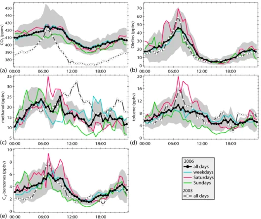
As expected, the compounds analyzed show a distinct diur-nal pattern with maximum concentrations during the morn-ing rush-hour period and minimum concentrations durmorn-ing the afternoon (see Fig. 2). The ambient concentrations in-crease sharply at 6 a.m., when the vehicular traffic begins. From 6 to 9 a.m. with a slowly growing boundary layer and weak photochemical activity, concentrations of primary pol-lutants reach maximum levels. After this period, the con-centrations of the primary pollutants decrease due to dilution within the growing boundary layer and photochemical reac-tions. At sunset, the development of a new nocturnal stable boundary layer enhances the accumulation of pollutants from the evening rush hour. A detailed description of the diurnal VOCs pattern in the atmosphere of Mexico City is provided by Velasco et al. (2007). The only exception to this descrip-tion is methanol, which does not decrease substantially dur-ing the day, suggestdur-ing a strong secondary formation durdur-ing the day or the mixing with air aloft enriched in methanol. Methanol has a long life time; consequently, emissions from biogenic and biomass burning sources outside of the city, both primary and secondary from oxidation processes may also be significant contributors (Jacob et al., 2005; Holzinger et al., 2005).

In general, the diurnal patterns of the species measured were relatively constant during the entire field campaign. Ta-ble 1 shows the 24-h median concentrations and the median concentrations measured during the morning rush-hour pe-riod (6–9 a.m.). Although the number of monitored week-ends was small (3), we found that the highest concentrations were observed on Saturdays, while the lowest concentrations occurred on Sundays. An interesting feature is that the early morning concentrations on Saturdays and Sundays were con-sistently higher than on weekdays. This effect has been ob-served also in the local air quality monitoring network for the ambient concentrations of CO and NOx(Stephens et al.,

2008), and it has been called the “party effect” because of its origin from the abundant social and entertainment activities during Friday and Saturday nights, which yield higher traffic levels.

As shown in Fig. 2, the diurnal distributions observed in 2003 were similar to those observed in 2006. In terms of magnitudes, the 2003 concentrations of the analyzed species were mostly within the one standard deviation range of the 2006 concentrations, except CO2, which showed much lower

concentrations in 2003 for all hours of the day except the morning rush hour. On average the CO2difference between

the two campaigns was 22 ppmv. As noted in the next sec-tion, the CO2 fluxes in 2003 and 2006 were quite similar

which suggests that the concentration differences were due to differences in CO2 background concentrations between the

two sites and the two different years.

3.2 Fluxes

3.2.1 Diurnal patterns

As shown in Fig. 3, the fluxes of the species analyzed were always positive on a diurnal average basis which indicates that the urban surface is always a net source. The high-est fluxes occurred during daytime and the lowhigh-est during the night. In contrast to the ambient concentration profiles, which depend on emissions, deposition, and chemical and meteorological processes, the flux profiles depend primarily upon deposition and emission rates from the underlying sur-face. Due to the urban location, emissions are predominantly from anthropogenic activities. As described previously, bio-genic sources were insignificant because of the scarce veg-etation within the monitored footprint. In particular, for the olefin fluxes, no correlations with temperature or solar radi-ation were observed. In the same context, the CO2 uptake

by the urban vegetation was not strong enough to offset the CO2flux from anthropogenic sources during daytime. Even

though the footprint for some nocturnal periods extended to the Chapultepec Park located 1.4 km to the northwest of the tower, CO2respiration from plants was not evident in the flux

profile. This was because according to the footprint model applied, the footprint peak during stable conditions at night was located approximately 500 m upwind of the tower and well within the urban (non-park) landscape.

The fluxes of CO2, olefins and C2-benzenes showed

sim-ilar diurnal atterns. The morning-start of the fluxes of these species occurred at 6 a.m., coinciding with the onset of the morning rush-hour period. During the rest of the morning and the first three hours of the afternoon the fluxes remained relatively constant. Table 1 shows the average of the fluxes measured between 7 a.m. and 3 p.m., as well as for the entire day.

During the rest of the afternoon and evening, the fluxes of CO2, olefins and C2-benzenes drop gradually, apparently as

a consequence of a shift in the wind direction. Throughout the morning and early afternoon hours, the wind blew mostly from the WNW–ESE sector, while for the rest of the after-noon winds blew from the ESE–SSE sector or the NW. Con-sidering the entire diurnal course, the fluxes coming from the SE-SW sector were consistently lower than the fluxes com-ing from the rest of the wind rose, as shown for CO2fluxes

in Fig. 4. This suggests a difference in the distribution of the emission sources within the footprint. The number of av-enues with heavy traffic is higher in the WNW-ESE sector than in the SE-SW sector as shown in Fig. 1b.

The fluxes of toluene and methanol showed a different di-urnal pattern compared to the pattern for CO2, olefins and

C2-benzenes. The fluxes of these two species show two

in-crements during the morning: the first occurs at the begin-ning of the morbegin-ning rush-hour period, and the second occurs at approximately 9:30 a.m. In the first increment, methanol and toluene fluxes increase by a factor of ∼1.7, while in the

Fig. 2. Average diurnal patterns of ambient concentrations of (a) CO2, (b) mix of olefinic VOCs detected by the FOS, (c) methanol, (d)

toluene, and (e) C2-benzenes for the entire study, weekdays, Saturdays and Sundays. The ambient concentrations measured in 2003 at

the CENICA site are included as reference. The grey shadows represent ±1 standard deviation from the total 2006 averages, and give an indication of the day-to-day variability in each phase of the daily cycle. The time scale corresponds to the local standard time.

second increment, fluxes increase by a factor of ∼2.2. The second peak at 9:30 a.m. is attributed to the beginning of commercial painting and other solvent uses. Subsequently, the fluxes remain high and constant until 6 p.m. Table 1 shows the average fluxes for this period and for the entire day. For the rest of the day and night, toluene and methanol fluxes decrease to low levels.

In terms of day of the week, the highest fluxes were ob-served on weekdays, and the lowest on Sundays. Table 4 shows the ratios between the fluxes measured on Saturdays and Sundays with the fluxes measured on weekdays for dif-ferent periods of the day. Fluxes on Saturdays were between 13% and 24% lower than during weekdays, while on Sun-days the fluxes of CO2, olefins and C2-benzenes were

be-tween 33% and 54% lower, and the fluxes of toluene and methanol were ∼66% lower. The “party effect” was clearly observed in the early morning fluxes of CO2, olefins and

C2-benzenes, which were 25% higher between midnight and

6 a.m. on weekends than on weekdays. This nighttime in-crease was not observed for toluene and methanol fluxes. On Saturdays during the morning and early afternoon, the fluxes of toluene and methanol were similar or higher than those on weekdays.

The 2006 fluxes of VOCs and CO2show similar diurnal

profiles to those observed in 2003, but with higher magni-tudes. The fluxes of CO2and olefins were 1.4 and 1.5 times

higher, respectively in 2006 than in 2003, mainly because traffic levels are higher near the 2006 site compared to the 2003 site. The number of congested roadways within the ob-served footprint in 2006 was at least twice as many as for the 2003 location. The fluxes of methanol and toluene were 2.6 and 1.7 times higher, respectively. We believe this was also due to differences in anthropogenic activities in the two neighborhoods. The C2-benzenes fluxes measured in 2006

were 2.6 times higher than those measured in 2003, thus we expected to find a similar relationship for CO2and olefins,

since C2-benzenes emissions also come from vehicular

com-bustion. An interesting feature in the 2003 flux profiles was a spike in the olefins flux during the morning rush-hour period. This spike was not observed in the olefins flux measured in 2006, nor in the fluxes of the other species measured in both years. This spike might arise from other local sources differ-ent than vehicle exhaust.

The spatial variability of VOC emissions within Mexico City was evaluated during the MILAGRO field campaign by DEC flux measurements of toluene and benzene from an

Fig. 3. Average diurnal patterns of the flux of (a) CO2, (b) mix of olefinic VOCs as propylene detected by the FOS, (c) methanol, (d) toluene,

and (e) C2-benzenes for the entire study, weekdays, Saturdays and Sundays. The fluxes measured in 2003 at the CENICA site are included

as reference. The grey shadows represent ±1 standard deviation from the total 2006 averages, and give an indication of the day-to-day variability in each phase of the daily cycle. The time scale corresponds to the local standard time.

Table 4. Ratios between the fluxes measured on Saturdays and Sundays and the fluxes measured on weekdays for different periods of the

day.

CO2 Olefins C2-benzenes Toluene Methanol

Sat. Sun. Sat. Sun. Sat. Sun. Sat. Sun. Sat. Sun. All day 0.76 0.49 0.87 0.67 0.86 0.46 0.80 0.32 0.78 0.35 0–6 a.m. 1.05 1.11 1.48 1.33 1.28 1.16 1.04 0.62 0.62 0.66 6 a.m.–3 p.m. 0.82 0.43 0.89 0.61 0.94 0.35 1.03 0.30 1.41 0.39 3 p.m.–12 a.m. 0.62 0.49 0.73 0.63 0.55 0.49 0.40 0.28 0.34 0.25 10 a.m.–3 p.m. 1.00 0.29 1.78 0.38

aircraft platform (Karl et al., 2009). These flights were car-ried out across the northeast section of the city where the industrial district and the airport are located. For these loca-tions, fluxes of toluene above 12 µg m−2s−1were observed, with a median flux of 3.9±1.1 µg m−2s−1 along the flight leg. This median flux is 1.3 times larger than the peak flux and 2.8 times larger than the average daytime flux observed at our ground site.

3.2.2 Correlation between fluxes of VOCs and CO2

Because of the close relationship between CO2and

combus-tion sources, comparison of the flux measurements of se-lected VOCs and CO2is useful in examining the origin of

those VOCs, as well as determining their emission rates in terms of the CO2released from the urban surface. Figure 5

shows the correlations between the fluxes of the analyzed VOC species, including benzene, and CO2. It is

Fig. 4. Histograms of wind direction during two diurnal periods,

7 a.m. to 3 p.m. (a), and 3 p.m. to 9 p.m. (b) for the entire field campaign. The color gradient indicates the CO2flux average for

each wind direction sector and diurnal period.

photochemical aging or meteorological processes, and ne-glecting the human and vegetation respiration, the correla-tions with CO2provide a basis for direct evaluation of the

emission rates from an urban district.

In this way, we found that olefins, benzene and C2

-benzenes appear to have their main origin in combustion sources. The variability on the emission ratios as a function of the period of the day shown in Fig. 5 is different for each compound, and it is also an indication of the variability of combustion sources. Benzene shows good flux correlations with CO2 throughout the day with high correlation

coeffi-cients ranging from 0.67 to 0.91, and low variability in the ra-tios throughout the day. From the correlation using the entire set of data, the monitored district emits 0.16 µg of benzene per mg of CO2. In the same context, 0.60 µg of both olefins

and C2-benzenes are emitted per mg of CO2. The

emis-sion relationship among compounds can vary considerably within the Mexican fleet, as observed during on-road VOC characterization of vehicle plumes during the MCMA-2003 field campaign (Zavala et al., 2006; Velasco et al., 2007) and MCMA-2006 (Zavala et al., 2009). This variation in the emission ratios from vehicle exhaust, in addition to evapora-tion from fuel tanks and engines, contributes to the scatter in the correlations between the fluxes of these species and CO2.

The variations of the FOS response to different alkenes may

also contribute to the scatter in the correlation between the fluxes of olefins and CO2.

The correlations between the fluxes of toluene and methanol with the fluxes of CO2show more scatter than the

correlations for the species and CO2mentioned above. These

two compounds are associated with solvent evaporation from cleaning, painting, and printing processes, as well as from application of adhesives, dyes and inks. During a portion of the field campaign, the evaporative emissions of these two species appeared to be strongly enhanced by the application of a paint resin to the sidewalks near the tower by the lo-cal district city maintenance workers. The intense fluxes of toluene and methanol appear to follow the schedule of the district workers, ending at 6 p.m. on weekdays and 3 p.m. on Saturdays. On weekdays from 9:30 a.m. to 6 p.m., the ratios between the fluxes of toluene and methanol relative to CO2

were 1.9 and 1.5 times higher, respectively, than during the rest of the day. Moreover, the flux ratio of 0.62 µg of toluene per mg of CO2for the rest of the day was essentially similar

to the ratio (0.63) observed at the CENICA site in 2003. To further investigate the sources of toluene, we exined the toluene to benzene ratio in terms of fluxes and am-bient concentrations (see Fig. 6). Since vehicular traffic is the main source of benzene in urban environments (Fortin et al., 2005), benzene has been used as a tracer to identify VOC sources in different studies (e.g., Barletta et al., 2005; Schnitzhofer et al., 2008). From previous ambient concen-tration measurements, a toluene to benzene mass ratio of 4.3±2.0 was determined for urban sites of Mexico City (Ve-lasco et al., 2007), and a ratio of 1.9 for the Mexican fleet emissions (Zavala et al. 2006). A direct comparison between these two ratios suggests that in addition to vehicle exhaust, there are other important sources of toluene in Mexico City. For the ambient concentrations measured in 2006, a ratio of 4.8±0.3 was found, similar to the ratio reported previously for other urban sites of the city. The neighborhood sidewalk resin application does not appear to affect the ratio for the 2006 measurements compared to the other measurements, as shown in Fig. 6a.

In contrast, the effect of the resin application is clearly observed in Fig. 6b for the ratio in terms of fluxes. Dur-ing the resin application, the mass ratio between fluxes was 7.0±1.2, approximately 1.7 times higher than during the rest of the day (4.2±0.5), when the ratio between fluxes was sim-ilar to the ratio observed for ambient concentrations. Karl et al. (2009) also observed the impact of evaporative emissions on the toluene to benzene ratio, for the northern industrial district they observed peak flux ratios ranging from 10 to 15, with a mean ratio of 3.2±0.5 along their flights.

Continuous long-path measurements of toluene and benzene by Differential Optical Absorption Spectroscopy (DOAS) have shown that photochemical aging at a local scale in Mexico City is negligible due to the direct influ-ence of the fresh emissions on the atmospheric concentra-tions (Velasco et al., 2007). An alternative explanation for the

Fig. 5. Flux correlations between CO2and olefins (a), methanol (b), benzene (c), toluene (d), and C2-benzenes (e). The correlations were

divided into bins of 3-h periods throughout the day. The ratios (m) and correlation coefficients (r) for each period are included in the panels. The black line indicates the regression line for all the data; their ratios and correlation coefficients are in larger fonts.

discrepancy between concentration and flux ratios of toluene to benzene may be that the footprint is larger for ambient concentrations than for fluxes, as explained by Vesala et al. (2008). These ratios used with the ratio for the Mexican

vehicle fleet, suggests that 27% of the toluene flux is due to vehicle exhaust during this period, while 45% of the toluene flux appears to be linked to traffic during the rest of the day.

Fig. 6. Correlations between toluene and benzene for ambient concentrations (a) and fluxes (b). The correlations were calculated for two

periods, one including the period of resin application to the sidewalks (9 a.m. to 6 p.m.), and the second for the remaining time. The black line indicates the regression line for all the data.

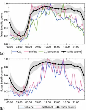
Fig. 7. Diurnal profiles of normalized traffic counts and fluxes of

CO2, olefins, and C2-benzenes (a), and toluene and methanol (b).

The traffic counts represent the average traffic from 11 roadways in a 10 km radius from the flux tower site. The gray shadow indi-cates ±1 standard deviation from the traffic counts. The time scale corresponds to the local standard time.

3.2.3 Fluxes as a function of vehicular activity

To evaluate the influence of the vehicular traffic on the emis-sions of these species we can compare flux measurements with traffic density data. For this comparison, we used traf-fic counts from 11 roadways in a 10-km radius from the flux tower. These traffic counts correspond to the most recent study (2003) of vehicular activity in the city carried out by the local authorities. The selected roadways are heavily trav-eled with traffic counts ranging from 14 875 to 68 171 vehi-cles daily. With the assumption that the diurnal traffic pattern has not changed significantly from 2003, each traffic count distribution was normalized to their maximum hourly count and the average from the 11 roadways is plotted along with the normalized fluxes in Fig. 7. The typical morning and af-ternoon traffic peaks are not identified, instead a single peak is observed during the entire day. This peak begins at 6 a.m., and extends until the evening. Figure 7a shows that the diur-nal flux patterns of CO2, olefins and C2-benzenes follow the

vehicular traffic profile during a large part of the day. The fluxes of these species and the traffic counts increase simul-taneously during the morning rush-hour period, and stay con-stant for the rest of the morning. Throughout the afternoon, the fluxes of these species drop gradually, but not the vehic-ular traffic. As discussed previously, this afternoon decrease in fluxes is due to a change in the wind direction toward a sector with lower traffic levels.

The morning and late afternoon offsets between the nor-malized profiles of traffic and toluene and methanol fluxes in Fig. 7b, show the impact of the evaporative emissions from the resin applied to the sidewalks near the tower from 9 a.m. to 6 p.m. Comparison of the correlation coefficients obtained from linear regressions between traffic counts and

Fig. 8. Comparison of the diurnal profiles of fluxes of CO₂(a), olefins (b), methanol (c), toluene (d), and C₂-benzenes (e) with the diurnal profiles of emissions from the 2006 emissions inventory. The emissions were extracted from the grid cells coinciding with the footprints described in the text and the 63 surrounding cells. The gray shadows indicate ±1 standard deviation of the measured fluxes.

fluxes of toluene (0.72) and methanol (0.73), with those ob-tained for CO2(0.94), olefins (0.91) and C2-benzenes (0.84)

confirms the lower vehicle exhaust contribution to toluene and methanol fluxes.

3.3 Comparison of measured fluxes versus calculated emissions in the local emissions inventory

A primary purpose of this work was to employ the flux data to evaluate the accuracy of the gridded emissions inventory derived for air quality modeling. To accomplish this, we compared our flux measurements to the most recent emis-sions inventory for Mexico City. This emisemis-sions inventory covers the entire metropolitan area in cells of 1 km2, with hourly emissions of CO2 and 552 VOC species, including

other pollutants from mobile, area and point sources, using 2006 base data (SMAGDF, 2008). This inventory was cre-ated using bottom-up methods and emission factors which were either measured locally or taken from the literature. For mobile sources, the MOBILE5 emissions model was adapted to account for local vehicle characteristics, and their emis-sions were distributed spatially and temporally on the basis of traffic count data for primary and secondary roadways.

Emissions from area sources were obtained from geographi-cal statistics, including population density, land use and eco-nomic level of each of the districts within the metropolitan area. Emissions from industries, workshops, and commerce and service establishments were obtained from operational permits containing information about their activities, such as processes, work hours, and location.

The CO2, olefins, toluene, C2-benzenes and methanol

emissions were extracted from the grid cells coinciding with the 5 footprints shown in Fig. 1a. The four 6-h foot-prints were averaged to obtain more precise emission profiles throughout the diurnal course. The emissions were adjusted by the footprint fraction covered in each cell (i.e., if the foot-print covered 47% of a cell, only 47% of the emissions from that cell were considered). In addition, the emissions from 63 cells around the flux tower were also extracted with the intent to analyze the homogeneity of the emissions over a wider area. Of these 63 cells, the mobile emissions from five cells appear to be incorrect. Three of them report very high emissions at nighttime, and the other two during daytime (be-tween 3 and 5 times higher than the maximum emissions re-ported for the other cells). The emissions from these cells were not included in the comparison. Their exclusion does

Fig. 9. Diurnal emission profiles distributed by source types for CO₂ (a), olefins (b), methanol (c), toluene (d), and C₂-benzenes (e). The emissions of CO2, olefins, toluene and C2-benzenes were extracted from the grid cells coinciding with the 6-h footprints obtained for

different periods of the diurnal course, while the methanol emissions represent the 63 surrounding cells. The black lines correspond to the average fluxes measured during the entire field campaign, while the dashed lines indicate ±1 standard deviation of the measured fluxes.

not modify significantly the emission profiles since they are not included in all the evaluated footprints.

The emissions of olefinic VOCs in the inventory were weighted by their sensitivity response to the FOS listed in Table 2. For the other olefin species, we assumed null re-sponses. Similarly, the C2-benzenes emissions correspond to

the sum of ethylbenzene, benzaldehyde and the three xylene isomers.

Figure 8 shows the diurnal profiles of the measured fluxes along with the emission profiles obtained from the aver-age footprint of the entire set of measured periods, the pro-file obtained from averaging the four 6-h footprints (diur-nal footprint), and the 63 surrounding cells. In general, the best agreement between the measurements and the emis-sions inventory occurred with the diurnal footprint, except for methanol, as discussed later. In terms of species, CO2and

olefins show the best agreement between calculated sions and measured fluxes. Figure 9 shows the diurnal emis-sions of CO2, olefins, toluene and C2-benzenes separated

by major emission sources using the diurnal footprint. For methanol, emissions are referenced with respect to the 63 surrounding cells. For all species, according to the emis-sions inventory, with the exception of methanol, the mo-bile sources are the major contributors, with contributions

of 87% for CO2, 74% for olefins, 84% for C2-benzenes, and

72% for toluene on a daily averaged basis. Among the mo-bile sources, gasoline motor-vehicles are the principal tributors, as shown in Fig. 9. These contributions are con-sistent with the results found in the previous sections, with the exception of toluene, for which the traffic contribution was found to be lower. With regard to methanol, the emis-sions inventory indicated that methanol is emitted primarily from point sources and the use of auto-care products, with almost negligible evaporative contributions from adhesives, inks, pesticides and other domestic products. The emissions inventory does not report any vehicular contribution, con-trary to results from other studies (Legreid et al., 2007) and our observed methanol correlations with CO2flux and

vehic-ular activity.

As mentioned before, the diurnal profiles of CO2 and

olefin emissions from the emissions inventory follow closely the diurnal profiles of the measured fluxes. The emissions in-ventory agrees with the measured fluxes of CO2and olefins

to within 10% and 20%, respectively. With the exception of the early morning period, the CO2and olefin emissions were

generally within the variability range of the measured fluxes. From midnight to 6 a.m., the emissions from the diurnal foot-print and the 63 surrounding cells were larger than measured

fluxes by factors of 2.3 and 1.7 for CO2and olefins,

respec-tively. This overestimation was due to 6 point sources with high emissions that were only included in the footprint dur-ing the stable nighttime period. Their contribution to the CO2

emissions is indicated in Fig. 9.

The human respiration is an additional CO2source not

ac-counted in the emissions inventory. Considering the local ambient conditions and average weight of a Mexican, we es-timate that a person exhales 596 g CO2per day, which when

multiplied by the population density showed that human res-piration may account for 9% of the measured fluxes. Dur-ing daytime, the human exhalation represents 6% of the CO2

emissions and this does not change the level of agreement be-tween measured fluxes and estimated emissions, but at night-time the human respiration could increase the over-prediction in the emissions inventory.

The species measured by PTR-MS and DEC show larger differences between measured fluxes and calculated emis-sions than for CO2and olefins. On a daily basis, the

emis-sions inventory overestimates the total C2-benzene flux by a

factor of 2.1 for the average flux, and by 1.3 for the upper limit of the flux measurements. For toluene, the emissions inventory overestimates the average toluene flux by a factor of 1.6, but the emissions inventory is within the upper limit of the flux measurements throughout the diurnal period.

The estimated C2-benzenes emissions show a similar peak

to the toluene emissions due to emissions from painting, cleaning and printing (see Fig. 9), but this was not apparent in the flux measurements. Between 9:30 a.m. and 8:30 p.m., when the emissions inventory reports these emissions, the C2-benzene emissions were 1.7 times higher than the upper

limit of the fluxes defined by one standard deviation of the measurements. With these evaporative emissions removed from the inventory, the emissions inventory matches the up-per limit of the fluxes during this up-period, with an average emission only 10% higher than the flux average. This ob-servation suggests that mobile emissions are overestimated, since all evaporative emissions cannot be removed from the emissions inventory. In addition, for the rest of the day, when the inventory reports no evaporative emissions, the vehicular emissions are also overestimated. Nevertheless an overesti-mation in both, evaporative and mobile emissions cannot be ignored.

Considering that 27% of the toluene flux is due to mo-bile emissions during the resin application on the sidewalks near the tower and 45% during the rest of the day, as de-termined from the toluene to benzene flux ratio, it is clear that the toluene contribution from gasoline vehicles is over-estimated in the emissions inventory. But it appears that the evaporative emissions are also overestimated. The toluene peak in the emissions inventory coincides with the observed peak in the flux measurements due to the resin application. However, if this resin had not been applied, the toluene over-estimation in the emissions inventory would be even larger.

The emissions inventory shows a second peak in toluene and C2-benzenes emissions from 5:30 to 8:30 p.m. This

evening peak corresponds to emissions from workshops, commerce and service establishments with a longer working schedule. However, the flux measurements of both species did not register this peak.

The similarity in the emissions profiles obtained for the 3 different footprints evaluated for CO2, olefins, toluene, and

C2-benzenes indicates that the emissions of these species

re-ported by the emissions inventory are homogeneously dis-tributed within the analyzed district. However, the methanol emissions extracted from the average and diurnal footprints are always close to the lower limit of the flux measurements with a daily underestimation of 73%. The emissions from the 63 surrounding cells include point sources whose emis-sions reduce the difference with the average flux measure-ments to 25% (see Fig. 8c). The origin of this underestima-tion appears to be the omission of methanol emissions from mobile sources or omission of point sources in the emissions inventory and less likely to the underestimation of evapora-tive emissions from households and lack of biomass burning emissions.

Overall, these results are consistent with the findings from the comparison between the 2003 flux measurements and the 2002 emissions inventory (Velasco et al., 2005a). For olefins, the estimated emissions were always within one standard de-viation range of the measured fluxes, as well as for toluene. As in 2006, the 2002 emissions inventory overestimated the C2-benzenes emissions by a factor of 2 on a daily basis. For

the location of the city in 2003, the emissions of toluene and C2-benzenes did not show the daytime peak from

evapora-tive emissions. Methanol and CO2were not specified in the

2002 emissions inventory; therefore a comparison was not possible.

Although these results do not address the full suite of VOC emissions, and together with the 2003 measurements, repre-sent only two locations of the city, overall the findings sug-gest that the emissions inventory is relatively accurate for CO2and olefins, but too high for C2-benzenes and toluene

and too low for methanol. It seems that the emissions in-ventory predicts correctly the emissions from combustion sources, but overestimates the evaporative emissions from area sources, such as workshops, commerce and service es-tablishments. These discrepancies can be expected for an urban area as diverse and as large as Mexico City, where the data to accurately determine the anthropogenic emissions is limited and comes from a multitude of sources.

Our results are consistent with those of Lei et al. (2007, 2008), who by indirect comparisons between modeled and observed ambient concentrations of VOCs from MCMA-2003 concluded that the emissions of olefins re-ported in the emissions inventory (for the years 2002 and 2004) are generally accurate, and the emissions of aromatics need to be adjusted by factors between 1 and 1.5 depend-ing on the compound. These finddepend-ings do not support the

suggestion that VOC emissions are underestimated by factors ranging from 3 to 4 by West et al. (2004) and Arriaga-Colina et al. (2004).

4 Conclusions

The urban flux system deployed in Mexico City as part of the MILAGRO/MCMA-2006 field campaign showed agreement with the flux measurements collected during the MCMA-2003 campaign from a different site within the city after accounting for differences in local traffic levels. The flux data collected in both studies indicate that the general con-straints with the EC methods are satisfied and also that the measured fluxes are representative of emissions on the same scale as the resolution of typical urban emission inventories. Together, the data show that the emissions inventory is in rea-sonable agreement with measured olefin and CO2fluxes, but

C2-benzenes and toluene emissions from gasoline vehicles

and evaporative sources are overestimated in the inventory. It appears that methanol emissions from mobile sources oc-cur, but are not included in the emissions inventory. These conclusions are valid for the monitored sites, discrepancies with the emissions inventory might occur for other sectors of the city, in particular for industrial areas.

The flux measurements presented here demonstrated that the EC technique coupled with fast response sensors can be used to evaluate directly emission inventories in a way that is not possible with other indirect evaluation methods, mak-ing it a new and valuable tool for improvmak-ing the air quality management process.

Acknowledgements. This study was supported by the National

Sci-ence Foundation (ATM-0528227), Department of Energy (Award DE-FG02-05ER63980), the Comisi´on Ambiental Metropolitana of Mexico and the Molina Center for Strategic Studies in Energy and the Environment. The assistance and logistical support provided by the Atmospheric Monitoring System of the Federal District Government (SIMAT) was instrumental for the satisfactory devel-opment of this study. The authors acknowledge the constructive comments from the anonymous reviewer and the editor.

Edited by: S. Madronich

References

Amman, C., Brunner, A., Spirig, C., and Neftel, A.: Technical note: water vapour concentration and flux measurements with PTR-MS, Atmos. Chem. Phys., 6, 4643-4651, 2006,

http://www.atmos-chem-phys.net/6/4643/2006/.

Aubinet, M., Grelle, A., Ibrom, A., Rannik, ¨U., Moncrieff, J., Fo-ken, T., Kowalsky, A. S., Martin, P. H., Berbigier, P., Bernhofer, Ch., Clement, R., Elbers, J., Granier, A., Gr¨unwald, T., Morgen-stern, K., Pilegaard, K., Rebmann, C., Snijders, W., Valentini, R., and Vesela, T.: Estimates of the annual net carbon and water exchange of forests: the EUROFLUX methodology, Adv. Ecol. Res., 30, 113–175, 2000.

Auble, D. L., and Meyers, T. P.: An open path, fast response in-frared absorption gas analyzer for H2O and CO2, Bound.-Layer

Meteorol. 59, 243–256, 1992.

Arriaga-Colina, J. L.,West, J. J., Sosa, G., Escalona, S. S., Ordu˜nez, R. M., and Cervantes, A. D. M.: Measurements of VOCs in Mex-ico City (1992–2001) and evaluation of VOCs and CO in the emissions inventory, Atmos. Environ., 38, 2523–2533, 2004. Barletta, B., Meinardi, S., Rowland, F. S., Chan, C.-Y., Wang, X.,

Zou, S., Chan, L.-Y., and Blake, D. R.: Volatile organic com-pounds in 43 Chinese cities, Atmos. Environ. 39, 7706–7719, 2005.

de Gouw, J. and Warneke, C.: Measurements of volatile organic compounds in the Earth’s atmosphere using proton-transfer-reaction mass spectrometry, Mass Spectrom. Rev., 26, 223–257, 2007.

Fast, J. D., de Foy, B., Acevedo Rosas, F., Caetano, E., Carmichael, G., Emmons, L., McKenna, D., Mena, M., Skamarock, W., Tie, X., Coulter, R. L., Barnard, J. C., Wiedinmyer, C., and Madronich, S.: A meteorological overview of the MILAGRO field campaigns, Atmos. Chem. Phys., 7, 2233–2257, 2007, http://www.atmos-chem-phys.net/7/2233/2007/.

Fortin, T. J., Howard, B. J., Parrish, D. D., Goldan, P. D., Kuster, W. C., Atlas, E. L., and Harley, R. A.: Temporal changes in U.S. benzene emissions inferred from atmospheric measure-ments, Environ. Sci. Technol., 39, 1403–1408, 2005.

Grimmond, C. S. B., King, T. S., Cropley, F. D., Nowak, D. J., and Souch, C.: Local-scale fluxes of carbon dioxide in urban envi-ronments: methodological challenges and results from Chicago, Environ. Pollut. 116, 243–254, 2002.

Grimmond, C. S. B. and Oke, T. R.: Aerodynamic properties of ur-ban areas derived from analysis of surface form, J. App. Meteor., 38, 1262–1292, 1999.

Grivicke, R., Jimenez, J. L., Nemitz, E., Alexander, L., Velasco, E., Allwine, G., Pressley, S., Jobson, T., Molina, L. T., and Lamb, B.: Aerosol concentrations and fluxes in urban Mexico City dur-ing MILAGRO 2006, in preparation, 2009.

Guenther, A. B. and Hills, A.: Eddy covariance measurement of isoprene fluxes, J. Geophys. Res., 103, 13145–13152, 1998. Holzinger, R., Williams, J., Salisbury, G., Kl¨upfel, T., de Reus, M.,

Traub, M., Crutzen, P. J., and Lelieveld, J.: Oxygenated compounds in aged biomass burning plumes over the Eastern Mediterranean: evidence for strong secondary production of methanol and acetone, Atmos. Chem. Phys., 5, 39–46, 2005, http://www.atmos-chem-phys.net/5/39/2005/.

Hsieh, C. I., Katul, G., and Chi, T.: An approximate analytical model for footprint estimation of scalar fluxes in thermally strat-ified atmospheric flows, Adv. Water Resour., 23, 765–772, 2000. Jacob, D. J., Field, B. D., Li, Q., Blake, D. R., de Gouw, J., Warneke, C., Hansel, A., Wisthaler, A., Singh, H. B., and Guenther, A.: Global budget of methanol: constraints from atmospheric observations, J. Geophys. Res., 110, D08303, doi:10.1029/2004JD005172, 2005.

Karl, T., Apel, E., Hodzic, A., Riemer, D. D., Blake, D. R., and Wiedinmyer, C.: Emissions of volatile organic compounds in-ferred from airborne flux measurements over a megacity, Atmos. Chem. Phys., 9, 271–285, 2009,

http://www.atmos-chem-phys.net/9/271/2009/.

Karl, T. G., Spirig, C., Rinne, J., Stroud, C., Prevost, P., Green-berg, J., Fall, R., and Guenther, A.: Virtual disjunct eddy