HAL Id: hal-00296155
https://hal.archives-ouvertes.fr/hal-00296155
Submitted on 22 Feb 2007
HAL is a multi-disciplinary open access
archive for the deposit and dissemination of
sci-entific research documents, whether they are
pub-lished or not. The documents may come from
teaching and research institutions in France or
abroad, or from public or private research centers.
L’archive ouverte pluridisciplinaire HAL, est
destinée au dépôt et à la diffusion de documents
scientifiques de niveau recherche, publiés ou non,
émanant des établissements d’enseignement et de
recherche français ou étrangers, des laboratoires
publics ou privés.
M. Keil, D. R. Jackson, M. C. Hort
To cite this version:
M. Keil, D. R. Jackson, M. C. Hort. The January 2006 low ozone event over the UK. Atmospheric
Chemistry and Physics, European Geosciences Union, 2007, 7 (3), pp.961-972. �hal-00296155�
www.atmos-chem-phys.net/7/961/2007/ © Author(s) 2007. This work is licensed under a Creative Commons License.
Chemistry
and Physics
The January 2006 low ozone event over the UK
M. Keil, D. R. Jackson, and M. C. Hort
Met Office, FitzRoy Road, Exeter, EX1 3PB, UK
Received: 7 July 2006 – Published in Atmos. Chem. Phys. Discuss.: 5 September 2006 Revised: 18 December 2006 – Accepted: 19 February 2007 – Published: 22 February 2007
Abstract. In this paper we present a case study of a record
low ozone event observed over the UK in January 2006. We focus on the dynamical processes that cause this event. This is done by examining the observations, meteorological anal-yses and back trajectories calculated by the NAME III atmo-spheric dispersion model. We show that this model, hitherto only used for tropospheric pollution studies, can be an im-portant and effective tool for the examination of transport in the upper troposphere/lower stratosphere (UTLS) and mid-stratosphere regions.
A record low total ozone column of 177 DU was observed at Reading, UK, on 19 January 2006. Low ozone values were also recorded at other stations in Northwest Europe around this date. Ozonesonde measurements indicate the depletion is occurring in two distinct vertical regions, with around a third of the reduction in total ozone column values originat-ing from the mid-stratosphere and the rest from the UTLS region. Evidence suggests that air inside the stratospheric polar vortex was poor in ozone prior to 19 January and the occurrence of a major stratospheric warming shifted this air over Northwest Europe. In addition we show that moderate ozone depletion, related to the lifting of the tropopause and divergence in the lower stratosphere associated with the pres-ence of an anticyclone, is also a plausible mechanism for the record low ozone column that is observed.
In order to confirm that both mid-stratosphere and UTLS transport processes are responsible for the record low ozone values, we perform turbulent back trajectory calculations us-ing the Met Office NAME III model. The results show that air parcels in the mid-stratosphere that arrive over the British Isles on 19 January originate in the polar vortex, and fur-thermore that air parcels near the tropopause arrive from low latitudes and are transported anticyclonically. Therefore this strongly suggests that the record low ozone values are due to a combination of a raised tropopause with increased di-vergence in the lower stratosphere and the presence of low ozone stratospheric air aloft.
Correspondence to: M. Keil
1 Introduction
In this paper we document the very low ozone event observed over the UK in January 2006, and investigate the dynamical processes that caused this event. It is not uncommon to ob-serve reductions in the total ozone column at such latitudes in winter, since it is well-known that column total ozone levels undergo fluctuations associated with the passage of tropo-spheric weather systems. Cases where depletion occurs are often referred to as “ozone mini-holes” and have been doc-umented by a number of authors e.g. Newman et al. (1988); McKenna et al. (1989); Peters et al. (1995); James (1998). Such mini-holes occur frequently in mid and high latitudes (James, 1998), but they are rarely as deep as the one that we choose to examine in this paper. Therefore, to begin with, we summarise the dynamical processes that are believed to cause moderate strength and intense mini-holes.
The ozone depletion observed in a mini-hole of moder-ate strength results from the presence of an anticyclone in the upper troposphere/lower stratosphere (UTLS). These an-ticyclones are present as a result of poleward Rossby-wave breaking events at mid latitudes. The associated raising of the tropopause means that a greater proportion of the col-umn is occupied by ozone-poor tropospheric air. In addi-tion, the divergence of ozone-rich air out of the column in the lower stratosphere leads to a further reduction in total ozone. This has been the subject of numerous studies. For exam-ple, James and Peters (2002) performed a Lagrangian study of mini-holes and showed the holes to be associated with anomalous warm anticyclonic flow in the upper troposphere. Koch et al. (2005) looked at potential vorticity composites of central European mini-holes. These highlighted the im-portance of long-range meridional transport in the formation of mini-hole, whilst local adiabatic vertical displacement of isentropes play an additional, less important role in mini-hole formation. Further studies, e.g. Hood and Soukharev (2005); Peters and Entzian (1999), have examined trends in total ozone in the northern hemisphere in recent decades, and have found that changes in UTLS dynamics and the Brewer-Dobson circulation have a strong influence on total ozone
decadal changes and, by implication, related trends in ozone mini-hole frequency.
As already stated, mini-holes of moderate strength occur frequently in mid and high latitudes (James, 1998), but a smaller number of very intense mini holes are often observed in combination with a sudden stratospheric warming or other distortion of the stratospheric polar vortex. In these events the air within the vortex is ozone-poor, due to the very cold temperatures within the vortex and the associated chemical destruction of stratospheric ozone. The horizontal advection of this ozone-poor air over a region where the ozone column is already reduced due to the presence of a UTLS anticyclone leads to an even larger reduction in the total ozone column. Case studies of such events include Petzoldt et al. (1994); Petzoldt (1999) and Allen and Nakamura (2002). The lat-ter reported a total ozone column of 165 DU on 30 Novem-ber 1999 over Europe observed by the Total Ozone Mapping Spectrometer (TOMS). This is a record for this instrument and this location. Allen and Nakamura used a tracer trans-port model to reconstruct the ozone field in November 1999 and thus to determine the mechanism that caused the very low ozone column over Europe.
The aim of this paper is to present a case study of a very low ozone event observed over the UK in January 2006. We first examine observations of this event and associated me-teorological analyses. These suggest that the low observed ozone is due to the simultaneous occurrence of the two pro-cesses listed above. First, ozone in the mid-stratosphere is depleted. This probably occurs because the stratospheric vor-tex (and the ozone-poor air within it) has been transported from high latitudes to over the UK in the week or so leading up to 19 January. Second, on 18 and 19 January, an anti-cyclone is present in the troposphere and lower stratosphere over the UK. The associated lifting of the tropopause and lower stratospheric divergence will lead to a lowering of the ozone column.
In order to seek confirmation that such transport is actually taking place, we perform turbulent back trajectory calcula-tions to determine the origin of the air arriving at Reading on 19 January, and the path that air took. These trajectories are calculated from the Met Office NAME III dispersion model (Ryall and Maryon, 1998; Jones et al., 2005). NAME III is a Lagrangian particle dispersion model which hitherto has primarily been used to investigate tropospheric pollution in a wide range of applications ranging from the dispersion of nuclear contamination and volcanic ash to the prediction of air quality levels based on thousands of UK and European anthropogenic and natural emissions. The results presented here show that the NAME III model can also be a very effec-tive tool for diagnosing events in the stratosphere.
This paper brings together information from a number of sources in order to investigate this unusual low ozone event. Most of the observation and analysis data presented here are freely available in the public domain, except for the NAME III runs. This paper demonstrates how events of this kind
can be quickly diagnosed without performing costly chem-ical transport model (CTM) runs. A full CTM representa-tion of this event would offer complementary informarepresenta-tion, but this is beyond the scope of this paper.
The outline of the paper is as follows. In Sect. 2 the low ozone event is described via UK ground-based total ozone measurements, hemispheric maps of World Meteorological Organisation (WMO) Ozone Mapping Centre total ozone, and ozonesonde profiles from Lerwick, UK. The meteoro-logical situation in the stratosphere and near the tropopause is described in Sect. 3 and is used to interpret the patterns shown in the ozone measurements. Then in Sect. 4 turbulent back trajectory calculations from the NAME III model are used to determine the origin of the air parcels that arrived at Reading on 19 January 2006. Conclusions appear in Sect. 5.
2 Observations of the low ozone event
We start by presenting observations made over the UK by
Dobson spectrophotometers at Lerwick (60.13◦N, 1.18◦W),
Camborne (50.13◦N, 5.18◦W) and Bracknell (51.38◦N,
0.78◦W) and by a Brewer spectrophotometer at Reading
(51.46◦N, 0.97◦W). The Lerwick observations used are
from January 1979–present, the Reading observations from January 2003–present, and the Camborne and Bracknell ob-servations are a combined dataset that spans November 1989 to December 2003.
The retrieval accuracy of the Dobson instrument is around
±1% in direct sun conditions. In this paper we focus on
Jan-uary, when the sun is low, and the observational accuracy for this period is ±4% (Komhyr, 1980). The retrieval accuracy of a well-maintained Brewer spectrophotometer is ±1% and its precision is better than ±1% (Gao et al., 2001).
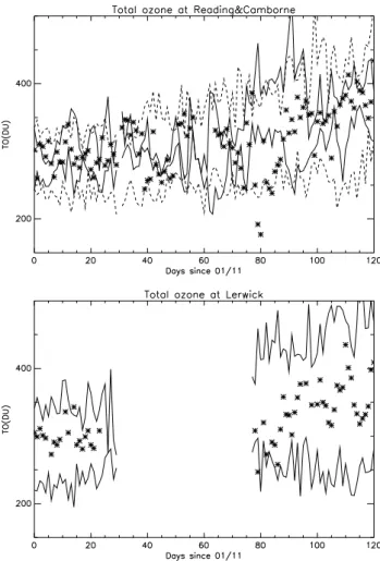
At Reading, like in much of the northern hemisphere, min-imum total ozone is observed between November and Febru-ary. Figure 1 (top panel) shows 2005/06 observations for these months and the daily maximum and minimum values from the 2002/03 to 2004/05 winters. The minimum value recorded is 177 DU on 19 January 2006. This is more than 100 DU less than the minimum for 19 January for the previ-ous observed winters and is also clearly less than the daily minimum for any other day in the November to February pe-riod (apart from the observation on 18 January 2006).
The dataset at Reading is too short to adequately repre-sent interannual variability and therefore to gain an indica-tion of this, we look at the daily maxima and minima from the 14 year long record from Camborne/Bracknell. These locations are sufficiently close to Reading for us to assume they approximately represent the 1989–2003 climatology for Reading. Figure 1 shows that the daily minimum for Cam-borne/Bracknell on 19 January is less than the 2002/03– 2004/05 daily minimum at Reading, but it is still over 50 DU greater than the observation at Reading on 19 January 2006.
The lower panel of Fig. 1 shows total ozone observations at
Lerwick, which is approximately 10◦latitude north of
Read-ing. It can be seen that the minimum total ozone for 2005/06 is observed on 18 January, one day before the minimum at Reading. Although this is a new low for the climatology en-velope for this date, this minimum is less remarkable as it is fairly similar to other daily minima from the 1979–2005 record.
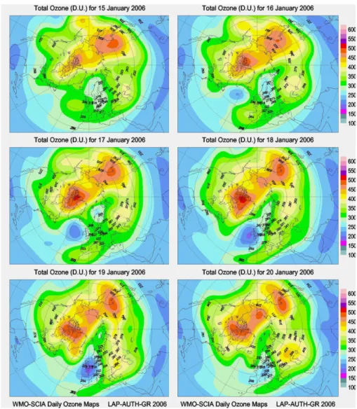
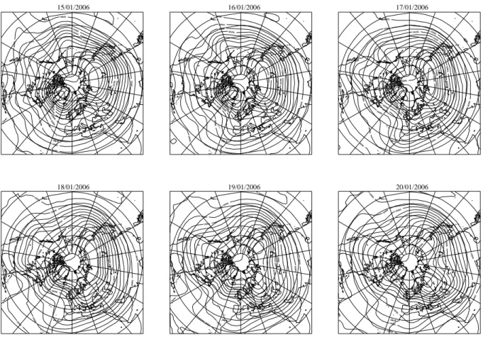
In order to gain a better idea of the spatial pattern of this total ozone event, we now look at daily maps of hemispheric total ozone. The maps are obtained from the WMO Ozone Mapping Centre (http://lap.physics.auth.gr/ozonemaps). The maps are created by assimilating total ozone data from the Scanning Imaging Absorption spectroMeter for At-mospheric CartograpHY (SCIAMACHY) using a transport model (Eskes et al., 2003). The transport model uses winds from European Centre for Medium Range Weather Fore-casts (ECMWF) analyses. The SCIAMACHY total ozone columns are retrieved using the TOSOMI algorithm, which is described by Eskes et al. (2005). Validation shows a bias of around −1.5% compared to Global Ozone Mapping Ex-periment (GOME) and ground-based observations.
Figure 2 shows daily WMO ozone maps from 15–20 Jan-uary 2006. Focusing on latitudes north of 45◦N, we see that for all days the lowest ozone values (<350 DU) are most fre-quently seen over a large region spanning the North East At-lantic and Northern Europe. An examination of geopotential height at 46 hPa and Ertel’s potential vorticity at 520 K from Met Office analyses shows that the stratospheric vortex has been displaced from the pole and is located at approximately the same place as this low ozone region. This suggests that stratospheric ozone depletion contributes to the low ozone values. However, within the North East Atlantic/Northern Europe low ozone region defined above there is further struc-ture, which is of synoptic scale. For example, on 17 January there are two regions of low ozone (<300 DU) over the North East Atlantic and northern Scandinavia with higher ozone in between. This suggests a further process is also acting to reduce total ozone. The synoptic pattern is indicative of a change in column ozone related to the passage of tropo-spheric weather systems.
To get a better idea of what is happening to the vertical distribution of ozone, we now move away from total col-umn observations to look at ozone profiles measured by a Met Office ozonesonde at Lerwick. The sonde is of the Elec-trochemical Concentration Cell (ECC) type. The total error for ECC sondes is estimated to be within −7% to +17% in the upper troposphere, ±5% in the lower stratosphere up to 10 hPa and −14% to +6% at 4 hPa (Komhyr et al., 1995). Er-rors are higher in the presence of steep ozone gradients and where ozone amounts are low.
During winter, the sonde usually makes one ascent per week. Figure 3 shows that on 18 January 2006 ozone mixing ratios between 50 and 10 hPa are around 3–3.5 ppmv. This is up to 2 ppmv less than corresponding values from
observa-Fig. 1. Total ozone observations between 1 November and 29
February. Top panel: observations at Reading between 1 November 2005 and 28 February 2006 (asterisks), daily maximum and min-imum total ozone at Reading from January 2003–February 2005 data (solid lines), daily maximum and minimum total ozone at Camborne/Bracknell from 1989–2003 data (dashed lines). Bot-tom panel: observations at Lerwick between 1 November 2005 and 28 February 2006 (asterisks), daily maximum and minimum total ozone at Lerwick from January 1979–February 2005 data (solid lines).
tions made on 4 and 11 January 2006 and also around 1 ppmv lower than the January climatology of Lerwick radiosonde ascents. Further evidence of stratospheric ozone loss on sim-ilar dates are also shown in Fig. 3 from ozonesonde pro-files from Sodankyl¨a, Finland (67.35◦N, 26.63◦E). Between
around 50 and 10 hPa the ozone profiles on 5 and 18 January at Sodankyl¨a are broadly similar to those on 4 and 18 Jan-uary, respectively, at Lerwick. At lower altitudes, at around 200–80 hPa, the ozone values at Lerwick are up to 1 ppmv lower than climatology for both 4 and 18 January.
It is thus evident from Fig. 3 that there are two distinct areas, the UTLS and the mid-stratosphere, with low ozone values over Lerwick on 18 January 2006. An analysis of the
Fig. 2. Total ozone maps from the WMO Ozone Mapping Centre for 15–20 January 2006.
Fig. 3. Ozone profiles measured by ozonesondes at Lerwick on the left hand plot and Sodankyl¨a, Finland, on the right hand plot. The red
line corresponds to 4 and 5 January 2006 for Lerwick and Sodankyl¨a, respectively, the green line 11 January 2006, the black line 18 January 2006. The January climatology of Lerwick radiosonde ascents is shown in blue on both plots (dashed represents ±1σ ). Units: ppmv.
Valid at 12 GMT Jan 18 2006 Valid at 12 GMT Jan 11 2006 Valid at 12 GMT Jan 25 2006 Valid at 12 GMT Jan 4 2006 Level: 520 K Level: 520 K Level: 520 K Level: 520 K H H L H 28 33 22 33 H L H L 32 12 34 25 L H L H 27 33 19 30 H L L H 32 28 29 30 L L H L 28 27 34 H H H 25 H 35 38 32 L H H 34 L 30 33 35 L L H 25 L 30 27 37 H H L 25 L 36 34 23 L H L 24 H 31 35 11 H L H 36 H 34 31 35 H L H 32 L 34 30 37 H H L 25 H 33 34 33 H H H 31 L 35 34 37 L L L 26 H 29 24 29 H H L 34 H 33 79 17 L H H 33 32 80 31 L H L H 25 78 30 80 H L H H 34 28 34 74 H H L L 34 34 30 30 L L H H 28 29 49 37 L H L L 27 33 28 30 L L L L 29 30 10 50 H H L H 80 34 14 35 H L H H 38 30 37 71 L H H H 31 79 35 36 L L H 7 28 78 L L L 33 29 29 L L H 15 6 64 72 L H L 36 34 13 H L H 31 29 34 H H L 41 31 13 H H L 30 78 29 H 20 L 32 5 H H 20 79 33 L H 2 35 H 25 9 L5 25 20 25 30 25 30 15 30 2025 30 25 15 20 20 30 15 25 30 25 15 15 2025 30 30 10 20 15 15 20 25 30 30 30 25 35 30 35 40 45 40 35 30 25 4555 55 45 35 30 60 35 65 40 30 45 30 35 40 50 60 30 30 35 35 35 30 70 70 60 25 30 50 35 20 60 70 7060 50 40 70 65 35 403530 60 15 30 30 30 35 10 15 20 25 30 30 20 10 15 20 10 25 25 15 15 2025 25 15 10 15 40 20 45 25 50 30 55 20 25 60 65 10 10 15 20 25 10 20 30 30 20 15 2025 30
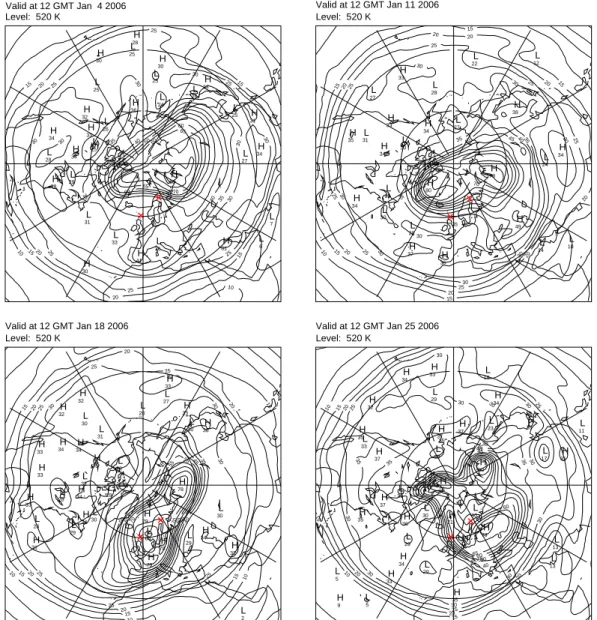
Fig. 4. PV on the 520 K theta surface (approx. 50 hPa) derived from Met Office analyses on 4 January 2006 (top left), 11 January 2006 (top
right), 18 January 2006 (bottom left), 25 January 2006 (bottom right). Contour interval 5 PV units. Crosses mark the locations of Lerwick and Sodankyl¨a.
Lerwick ozone profile data was performed in order to assign values to the amount of depletion from these two vertical re-gions. The profiles were split into two at 65 hPa and the sepa-rate areas were compared with the January climatology. The depletion attributed to each of these layers (surface to 65 hPa and 65 hPa to 10 hPa) was calculated in terms of total column ozone. The results reveal that approximately a third (34%) of the depletion in the total ozone column (w.r.t the January cli-matology) originates from the mid-stratospheric 65–10 hPa region, while two thirds (66%) comes from the UTLS region (note that the climatology and daily profiles are very similar for the majority of the troposphere). This analysis confirms that important ozone depleting processes occur in two dis-tinct regions and they are discussed further in Sect. 3.
3 Meteorological situation
In this section we use daily Met Office stratospheric analyses (Swinbank et al., 2004) to describe the meteorological situa-tion in January 2006. Unlike the cold, undisturbed Northern Hemisphere winter of 2004/5, the stratosphere has been dy-namically disturbed in 2005/6. In mid January there was a minor stratospheric warming, which became a major warm-ing on 21 January and persisted until early February. A ma-jor stratospheric warming occurs when the temperature
gra-dient at 10 hPa (around 30 km) between 60◦N and the pole
is reversed to become warmer towards the pole. In addition the zonal mean polar night jet reverses from westerly to
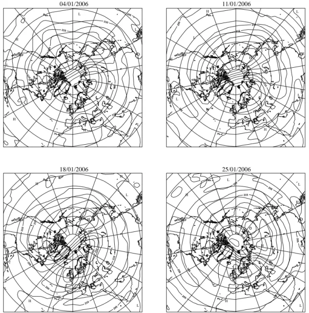
H H H H L L L L L 200 205 205 210 210 210 210 215 215 220 220 225 H H H H H H L L L L L 205 205 205 205 205 205 210 210 04/01/2006 18/01/2006 25/01/2006 11/01/2006 210 215 215 220 220 225 230 H H H H H L L L L L 200 205 205 205 205 205 210 210 210 210 215 215 220 225 H H H H H L L L L L L 205 205 205 205 205 205 205 210 210 210 215 215 220 220 225 225 230
Fig. 5. Temperature at 46 hPa from Met Office analysis on 4 January 2006 (top left), 11 January 2006 (top right), 18 January 2006 (bottom
left), 25 January 2006 (bottom right). Contour interval 5 K.
January 2006 major warming are greater than average. The typical meteorological situation for a cold, undis-turbed, January (such as in 2005) is a near-zonally symmetric polar vortex, centred near the pole and with associated cold temperatures. The analyses from January 2006 show a very different picture. Figure 4 shows Ertel’s potential vorticity on the 520 K isentropic surface (approximately 50 hPa) for selected days in January 2006. The impact of the January 2006 warming is a significant displacement of the polar night vortex away from the pole. During the course of the month the vortex becomes increasingly distorted and moves south-wards and eastsouth-wards across the North Atlantic and Northern Europe.
The southward movement of the vortex also implies south-ward movement of the cold air within it. This is reflected in
Fig. 5 which is similar to Fig. 4, except that temperatures at 46 hPa are shown. By 18 January minimum temperatures of less than 195 K are located over the British Isles. From then until 25 January this cold air is transported eastward across the British Isles and into central Europe. The Met Of-fice analyses show that the temperature in the polar vortex had fallen below the critical threshold for type I PSC for-mation (195 K at 46 hPa) in 22 of the 31 days prior to the observed event on 19 January. PSCs at similar locations are also seen in SCIAMACHY observations (von Savigny et al., 2005) on these days (data available from: http://www-iup.
physik.uni-bremen.de/∼sciaproc/PSC/PSC 2006 S00.html).
The low temperatures and the presence of PSCs during De-cember and January indicate that the air within the polar vor-tex is likely to be ozone poor for at least a week prior to 18
15400. 15500. 15600. 15600. 15700. 15700. 15800. 15800. 15900. 15900. 16000. 16000. 16100. 16100. 16100. 16200. 16200. 16200. 16300. 16300. 16300. 16400. 16400. 16400. 16500. 16500. 16500. 15200. 15300. 15400. 15/01/2006 16/01/2006 17/01/2006 18/01/2006 19/01/2006 20/01/2006 15500. 15600. 15700. 15700. 15800. 15800. 15900. 15900. 16000. 16000. 16100. 16100. 16200. 16200. 16200. 16300. 16300. 16300. 16400. 16400. 16400. 16500. 16500. 16500. 15200. 15300.15400. 15500. 15600. 15700. 15700. 15800. 15800. 15900. 15900. 16000. 16000. 16100. 16100. 16200. 16200. 16200. 16300. 16300. 16300. 16400. 16400. 16400. 16500. 16500. 16500. 15300. 15400. 15500. 15600. 15700. 15700. 15800. 15800. 15900. 15900. 16000. 16000. 16100. 16100. 16100. 16200. 16200. 16300. 16300. 16400. 16400. 16400. 16500. 16500. 16500. 15400. 15500. 15600. 15700. 15700. 15800. 15800. 15900. 15900. 16000. 16000. 16100. 16100. 16200. 16200. 16300. 16300. 16300. 16400. 16400. 16400. 16500. 16500. 16600. 15400. 15400. 15500. 15600. 15700. 15700. 15800. 15800. 15900. 15900. 16000. 16000. 16100. 16100. 16200. 16200. 16200. 16300. 16300. 16300. 16400. 16400. 16400. 16500. 16500. 16500.
Fig. 6. Geopotential height at 100 hPa from Met Office analyses on 15 January 2006 (top left), 16 January 2006 (top centre), 17 January 2006
(top right), 18 January 2006 (bottom left), 19 January 2006 (bottom centre) and 20 January 2006 (bottom right). Contour interval: 10 dam.
January. This is confirmed by a comparison of Figs. 3 and 4. Figure 4 suggests that both Lerwick and Sodankyl¨a are inside the polar vortex on 18 January and outside it on 4 January (on 11 January, Lerwick is outside the vortex and Sodankyl¨a is on the edge of the vortex). Figure 3 shows that mid stratosphere ozone at these sites is less when the observations are made in-side the vortex than outin-side the vortex. Thus, the low ozone air observed at Lerwick on 18 January is very likely a result of Lerwick being inside the polar vortex on that date. Maps of Ertel’s potential vorticity also show that Reading is within the stratospheric polar vortex on 19 January (not shown) and so it appears that the presence of ozone poor stratosphere vortex air also contributes to the record low ozone column observed at Reading on that date.
Some of the ozone depletion at Lerwick on 18 January is probably due to local heterogeneous chemical destruction associated with the presence of the PSCs implied by Fig. 5, rather than by the transport of pre-existing ozone-poor air to Lerwick. A quantification of the relative contributions of both these processes requires detailed chemical modelling studies, which are outside the scope of this study.
As indicated in Sects. 1 and 2, another mechanism for a re-duction in total ozone column is the raising of the tropopause
associated with the passage of anticyclones. Figure 6 shows geopotential height at 100 hPa from Met Office analyses for 15–20 January 2006. Focusing on the middle latitudes be-tween the central North Atlantic and Russia, we see that there is a clear link between anticyclones (cyclones), which can be seen as ridges (troughs) in Fig. 6, and depletions (enhance-ments) in the SCIAMACHY total ozone columns (Fig. 2). In addition, these features can also be associated with the surface pressure fields (not shown). In particular, the strong ridging pattern in the 100 hPa geopotential height fields can be related to large surface high pressure systems.
The origin of the ozone minimum over the British Isles on 19 January is seen on 16 January. On that date there are ozone minima (see Fig. 2) over the central North Atlantic and Scandinavia which are associated with anticyclones (Fig. 6) in these regions. The Atlantic anticyclone moves eastward over the next few days, reaching the British Isles on 19 Jan-uary, and the associated eastward movement of the ozone minimum can be seen in Fig. 2. By 20 January a low pres-sure system appears to the north of the British Isles, with an associated rise in ozone column (seen as a trough in Fig. 6). In subsequent days there is a continued fall/rise in to-tal ozone over the British Isles associated with the passage of
anticyclones/cyclones, but the very low ozone column seen on 18 and 19 January is not observed again.
The passage of anticyclones and the associated raising of the tropopause leads to net divergence in the stratospheric air aloft, thus removing relatively ozone rich air from the col-umn. A simple analysis of the stratospheric air above Read-ing on 18 January confirms that net divergence takes place in the 100–10 hPa column.
Similar synoptic situations to those described are seen in the Met Office 100 hPa geopotential height fields in early
January 2006. However, it is interesting that the
SCIA-MACHY fields do not show such a deep minimum in total ozone on these dates. This is confirmed by the ground-based observations in Fig. 1. This suggests that the very low ozone columns on 18 and 19 January are due to a combination of the presence of a UTLS anticyclone and of ozone depletion aloft.
4 NAME III model simulations
In this section we use the Met Office’s dispersion model, NAME III, to obtain further confirmation of the transport processes responsible for the low ozone event over the UK. NAME III is a Lagrangian particle dispersion model (Ryall and Maryon, 1998; Jones et al., 2005) within which emis-sions from pollutant sources are represented by particles re-leased into a model atmosphere. The particles are then ad-vected by the mean winds as calculated by the Met Office’s numerical weather prediction model, the Unified Model (Davies et al., 2005). Turbulent diffusion of the particles is modelled through the application of various random walk techniques (Rodean, 1996). Parameterizations also repre-sent processes such as the entrainment between the boundary layer and the free troposphere, the mixing by deep convec-tion, both wet and dry deposiconvec-tion, sedimentation and chemi-cal destruction and creation. The model is routinely used in a wide range of applications: examples include the prediction of air quality levels based on thousands of UK and European anthropogenic and natural emissions, the transport and depo-sition of debris following the Chernobyl accident (Smith and Clark, 1989) and the airborne spread of foot and mouth dis-ease during the epidemic in the UK in 2001 (Gloster et al., 2001).
In addition, a key advantage of utilizing a Lagrangian approach for dispersion modelling is the ability to run the model backwards in time. In this configuration particles are ’released’ from the receptor location and the resulting plots show where the air came from to arrive at the receptor. This enables sources to be identified from receptor data (Manning et al., 2003). Here, NAME III employs full turbulent trans-port and dispersion, referred to here as turbulent trajectories for simplicity. This requires that thousands of model parti-cles be released which results in the identification of source areas rather than points, as is the case with the more simple
back trajectory approach. This capability makes it possible to identify the origin or origins (both time and location) of the air reaching a location at any given time.
Simulations with the NAME III model were run to investi-gate the origins of the air contributing to the low ozone event over Reading on 19 January. Accordingly, a receptor was de-fined corresponding to the centre of the observed low ozone region, at 51.46◦N 0.97◦W, on that date. Simulations were run backwards in time for 5 days from this date, providing maps of the origin/path of the air arriving at this location. NAME III was driven by the analysis fields from the Met Office operational global weather prediction model, with the top of the domain being restricted to 30 km.
In order to assist in understanding the results a series of simulations were carried out using a receptor measuring
100 km2in the horizontal and extending from 10 km to 30 km
in altitude. The receptor was then repositioned at 5 different horizontal locations (North, South, East, West and Central) covering the extent of the observed low ozone feature. Re-sults for all the different horizontal locations are very consis-tent. This indicates that, over an area of 10◦in latitude and longitude centred at 51.46◦N 0.97◦W (the low ozone area), the simulations are spatially robust. Accordingly, all plots included here are for the central location.
NAME III results are presented in Figs. 7 to 10. These figures show where air arriving at the receptor on 19 January 2006 between 11:00:00 and 13:00:00 UTC originated from and passed through during a five day period preceding this time. The contours represent the time integrated air concen-tration from each model output grid box (dx,dy,dz) that con-tributes to the receptor. Each of the figures shows only the air that originated/passed through a certain depth of the at-mosphere to arrive at the receptor. In all cases the receptor’s size and location is the same.
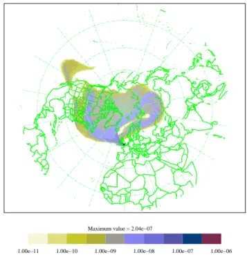
Figure 7 shows the air origin map for air originating over the whole vertical extent of the model i.e., 0–30 km. Much of the air mass arriving at the receptor originates in an area between Iceland and North West Russia. Comparisons with Met Office stratospheric Ertel’s potential vorticity maps for January (Fig. 4) suggest that this flow is very similar to the flow of the stratospheric polar vortex. In order to better deter-mine the origins of the air, further plots are shown which only show air arriving at the receptor that has originated/passed through certain atmospheric layers. Figure 8 is similar to Fig. 7, except that it only shows air arriving at the recep-tor that has originated/passed through a layer extending from 15–30 km. This confirms that the air originating between Ice-land and North West Russia is stratospheric in origin.
Figure 7 also shows air originating from other locations, such as the Pacific and the northern subtropical Atlantic. Fig-ure 8 shows that little or none of this air originates from the 15–30 km layer, so in order to determine the origin of this air, further vertical slices at 10–15 km and 5–10 km were ex-amined, and these are shown in Figs. 9 and 10, respectively. Both plots show that a proportion of the air arriving at the
1.00e−11 1.00e−10 1.00e−09 1.00e−08 1.00e−07 1.00e−06 Maximum value = 1.24e−07
Fig. 7. NAME III derived five day air history map for parcels
orig-inating in or passing through the 0–30 km vertical region from a receptor of 100 km2horizontal area with a 10–30 km vertical extent centred on 51.46◦N, 0.97◦W (black cross). The contours represent the time integrated air concentration from each grid box (dx,dy,dz) that contributes to the receptor on 19 January 2006 between 11:00 and 13:00 UTC given a release rate of 1 g/s.
receptor has travelled from the equatorial western Atlantic with a considerable northward component. It should be re-membered that for air to appear in any of the plots it must arrive at the receptor location at an altitude of 10–30 km. Therefore, Fig. 10 also indicates that some of the air arriv-ing at the receptor has ascended from the 5–10 km layer.
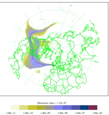
Figure 9 indicates that most of the air originating from the 10–15 km layer that subsequently arrives at the receptor lo-cation is not polar vortex in origin. The flow is very simi-lar in pattern to the geopotential height fields at 100 hPa in Fig. 6 and, close to the receptor, the trajectories follow an anti-cyclonic path. Figure 10 shows that there is also a vol-ume of air originating in the northern subtropical Atlantic from an altitude between 5 km and 10 km that took 3–5 days to arrive at the receptor location. This air also follows an anti-cyclonic path close to the receptor region.
We can see from Figs. 7–10 that air arriving at the receptor region has two main sources. Air originating from the 15– 30 km region is primarily stratospheric vortex in origin, with very little transport from elsewhere. In the previous section we showed that this air is likely to be ozone poor prior to arriving over the British Isles on 18 and 19 January.
The air arriving at the receptor from the 5–10 km and 10– 15 km layers is likely to have undergone horizontal and
ver-1.00e−11 1.00e−10 1.00e−09 1.00e−08 1.00e−07 1.00e−06 Maximum value = 2.04e−07
Fig. 8. As previous figure, except results are shown for air
originat-ing from or passoriginat-ing through the 15–30 km vertical region.
tical transport related to the passage of cyclones and anticy-clones shown in Fig. 6. Close to the receptor, the flow regime is anticyclonic which is consistent with a raised tropopause and divergence in the lower stratosphere. Accordingly, this leads to a decrease in the total ozone column. The results also show transport from low latitudes and low levels (see Fig. 10). However, the NAME III results by themselves can-not tell us whether this will lead to a further decrease, or an increase, in the ozone column at the receptor. These re-sults were in agreement with other NAME III runs based on receptor regions for the low ozone area on 17 and 18 Jan-uary, which showed air transported to the receptor region from similar areas.
5 Conclusions
A record low total column ozone value of 177 DU was ob-served at Reading, UK on 19 January 2006. In addition, ozonesonde observations from Lerwick show a large de-pletion in mid-stratospheric ozone between 50 and 10 hPa around this date, together with a noticeable decrease in the ozone around the UTLS, 200–80 hPa, region. Analysis of the ozonesonde data indicates that around one third of the de-pletion in the total ozone column originates from the middle stratosphere, and the rest is caused by the reduction in UTLS ozone values. This indicates that important ozone depleting processes were at work in two different regions.
Met Office analyses show that at this time the stratospheric polar vortex was displaced over the British Isles. Evidence
1.00e−11 1.00e−10 1.00e−09 1.00e−08 1.00e−07 1.00e−06 Maximum value = 1.32e−07
Fig. 9. As Fig. 8, except results are shown for air originating from
or passing through the 10–15 km vertical region.
10 30 50 70
80 60 40 20 0 20
1.00e−11 1.00e−10 1.00e−09 1.00e−08 1.00e−07 1.00e−06 Maximum value = 2.90e−08
Fig. 10. As Fig. 8, except results are shown for air originating from
or passing through the 5–10 km vertical region.
from Lerwick and Sodankyl¨a ozonesondes, and Met Office fields of Ertel’s potential vorticity, suggests that the British Isles was beneath the stratospheric vortex at this time and that the air within the vortex was already ozone poor. This low ozone air contributes to the record low ozone column
ob-served at Reading. The temperatures within the vortex were low enough to cause PSC formation and thus local ozone de-struction via heterogeneous chemistry, and it is a possibility that this could further add to the ozone depletion. However, without using a chemical model it is impossible to quantify how much ozone depletion could come from this source.
WMO total ozone maps show a large region of low ozone over the North East Atlantic and Northern Europe which is approximately colocated with the displaced polar vor-tex. However, superimposed on this low ozone region is a smaller, synoptic, scale pattern of middle latitude ozone column depletion. This points to another cause for the low ozone over the British Isles, namely the impact of anticy-clones in reducing the total ozone column. These events are well documented, see e.g. Newman et al. (1988); McKenna et al. (1989); Peters et al. (1995); James (1998), and fre-quently observed. They occur because associated with the presence of the anticyclone is a raising of the tropopause, meaning that a greater proportion of the column is occupied by ozone-poor tropospheric air. In addition, the divergence of ozone-rich air out of the column in the lower stratosphere leads to a further reduction in total ozone. We have shown that there is a strong link between the patterns of total ozone minima seen in the WMO maps and the location of anticy-clones in 100 hPa geopotential height fields from Met Office analyses. Therefore, it appears that this mechanism also con-tributes to the record low ozone columns observed.
In order to confirm the existence of these mechanisms we perform back trajectory calculations using the NAME III model. The receptor point for the trajectories was Reading. The results show that middle stratosphere air has been trans-ported in the polar vortex from higher latitudes from the re-gion of lowest temperatures, and this adds further weight to the hypothesis that this air will have undergone ozone de-struction due to heterogeneous chemistry prior to reaching the region of observed low ozone in mid latitudes. The model results also show that air transported from near-tropopause levels (5–15 km) arrives at the receptor point in an anticy-clonic path. This pattern is consistent with what is shown in Met Office analyses of geopotential height at 100 hPa and WMO total ozone maps, and also with previous trajectory-based studies of ozone miniholes over Europe, e.g. Koch et al. (2002). It clearly confirms that the synoptic scale re-ductions in ozone seen in these maps is associated with the raising of the tropopause and lower stratospheric divergence that occurs in the presence of these anticyclones.
It is important to note the possible health impacts of such decreased ozone events. Austin et al. (1999) reported record low ozone in late April/early May 1997 over southern Eng-land. The erythemally-weighted ultraviolet levels recorded at this time were similar to those normally recorded in June or July, and the impacts on human health of exposure to this ab-normally high amount of radiation are clear. Similarly, Stick et al. (2006) reported unusually large UV values over north-ern Germany in May 2005 as a result of an ozone mini-hole.
The event in January 2006 that we have reported may have some impact on the biosphere, but is unlikely to have many consequences for human health since erythemally-weighted ultraviolet levels do not usually start to become significant at middle or high latitudes until around a month after the spring equinox.
Acknowledgements. The authors would like to thank H. Eskes
from KNMI for the provision of assimilated ozone fields to the WMO ozone mapping centre. D. Moore provided Met Office ozonesonde data and his knowledge of the observations was extremely helpful. Sodankyl¨a ozonesonde data were obtained from the NILU database. Netcen provided the UK surface observations from Reading and Lerwick on behalf of DEFRA. Comments from the referees and a number of Met Office colleagues resulted in considerable improvements to this study.
Edited by: H. Wernli
References
Allen, D. R. and Nakamura, N.: Dynamical reconstruction of the record low column ozone over Europe on 30 November 1999, Geophys. Res. Lett., 29, 1362, doi:10.1029/2002GL014935, 2002.
Austin, J., Driscoll, C. M. H., Farmer, S. F. G., and Molyneux, M. J.: Late spring ultraviolet levels over the United Kingdom and the link to ozone, Ann. Geophys., 17, 1199–1209, 1999,
http://www.ann-geophys.net/17/1199/1999/.
Davies, T., Cullen, M. J. P., Malcolm, A. J., Mawson, M. H., Stan-iforth, A., White, A. A., and Wood, N.: A new dynamical core for the Met Office’s global and regional modelling of the atmo-sphere, Q. J. R. Meteorol. Soc., 131, 1759–1782, 2005. Eskes, H. J., van Velthoven, P. F. J., Valks, P. J. M., and Kelder,
H. E.: Assimilation of GOME total ozone satellite observations in a three-dimensional tracer transport model, Q. J. R. Meteorol. Soc., 129, 1663–1681, 2003
Eskes, H. J., van der A, R. J., Brinksma, E. J., Veefkind, J. P., de Haan, J. F., and Valks, P. J. M.: Retrieval and validation of ozone columns derived from measurements of SCIAMACHY on En-visat, Atmos. Chem. Phys. Discuss., 5, 4429–4475, 2005, http://www.atmos-chem-phys-discuss.net/5/4429/2005/. Gao, W., Slusser, J., Gibson, J., Scott, G., Bigelow, D., Kerr, J., and
McArthur, B.: Direct-Sun column ozone retrieval by the ultravi-olet multifilter rotating shadow-band radiometer and comparison with those from Brewer and Dobson spectrophotometers, Appl. Opt., 40, 3149–3155, 2001.
Gloster J., Champion H. J., Mansley L. M., Romero P., Brough, T., and Ramirez A.: The 2001 epidemic of foot-and-mouth dis-ease in the United Kingdom: epidemiological and meteorologi-cal case studies, The Veterinary Record, 156, 793–803, 2001. Hood, L. L. and Soukharev, B. E.: Interannual variations of total
ozone at Northern midlatitudes correlated with stratospheric EP flux and potential vorticity, J. Atmos. Sci., 62, 3724–3740, 2005 James, P. M.: A climatology of ozone mini-holes over the northern
hemisphere, Int. J. Climatology, 18, 1287–1303, 1998.
James, P. M. and Peters, D.: The Lagrangian structure of ozone mini-holes and potential vorticity anomalies in the Northern Hemisphere, Ann. Geophys., 20, 835–846
Jones, A., Thomson, D., Hort, M., and Devenish, B.: The U. K. Met Office’s next generation atmospheric dispersion model NAME III, Air pollution modeling and its application XVII, edited by: Borrego, C. and Norman, A., 580–589, Springer, 2007. Koch, G., Wernli, H., Staehelin, J., and Peter, T.: A Lagrangian
analysis of stratospheric ozone variability and long-term trends above Payerne (Switzerland) during 1970–2001, J. Geophys. Res., 107, 4373, doi:10.1029/2001JD001550, 2002.
Koch, G., Wernli, H., Schwierz, C., Staehelin, J., and Peter, T.: A composite study on the structure and formation of ozone mini-holes and minihighs over central Europe, Geophys. Res. Lett., 32, L12810, doi:10.1029/2004GL022062, 2005.
Komhyr, W. D.: Ozone Observations with a Dobson Spectropho-tometer, WMO Global Ozone Research and Monitoring Project Report No. 6, NOAA Environmental Research Laboratories, 1980.
Komhyr, W. D., Barnes, R. A., Brothers, G. B., Lathrop, J. A., and Opperman, D. P.: Electrochemical Concentration Cell ozonesonde performance evaluation during STOIC 1989, J. Geo-phys. Res., 100, 9231–9244, 1995.
Manning, A. J., Ryall, D. B., Derwent, R. G., Simmonds, P. G., and O’Doherty, S.: Estimating European emissions of ozone-depleting and greenhouse gases using observations and a mod-elling back-attribution technique, J. Geophys. Res., 108, 4405, doi:10.029/2002JD002312, 2003.
McKenna, D. S., Jones, R. L., Austin, J., Browell, E. V., Mc-Cormick, M. P., Krueger, A. J., and Tuck, A. F.: Diagnostic studies of the Antarctic vortex during the 1987 Airborne Antarc-tic Ozone Experiment – ozone miniholes, J. Geophys. Res., 94, 11 641–11 668, 1989.
Newman, P. A., Lait, L. A., and Schoeberl, M. R.: The morphol-ogy and meteorolmorphol-ogy of southern-hemisphere spring total ozone mini-holes, Geophys. Res. Lett., 15, 923–926, 1988.
Peters, D., Egger, J., and Entzian, G.: Dynamical aspects of ozone mini-hole formation, Meteorol. Atmos. Phys., 55, 205– 214, 1995.
Peters, D. and Entzian, G.: Longitude-dependent decadal changes of total ozone in boreal months during 1979–1992, J. Climate, 12, 1038–1048
Petzoldt, K., Naujokat, B., and Neugeboren, K.: Correlation be-tween stratospheric temperature, total ozone, and tropospheric weather systems, Geophys. Res. Lett., 21, 1203–1206, 1994. Petzoldt, K.: The role of dynamics in total ozone deviations from
their long-term mean over the Northern Hemisphere, Ann. Geo-phys., 17, 231–241, 1999,
http://www.ann-geophys.net/17/231/1999/.
Rodean, C.: Stochastic Lagrangian models of turbulent diffusion, Am. Met. Soc. Meteorological Monographs, 26(48), 1996. Ryall, D. B. and Maryon, R. H.: Validation of the UK Met. Office’s
NAME model against the ETEX dataset (1998), Atmospheric Environment, 32, 4265–4276, 1998.
Stick, C., Kr¨uger, K., Schade, N. H., Sandmann, H., and Macke, A.: Episode of unusually high solar ultraviolet radiation over central Europe due to dynamical reduced total ozone in May 2005, At-mos. Chem. Phys., 6, 1771–1776, 2006,
Smith, F. B. and Clark, M. J.: The transport and deposition of airborne debris from the Chernobyl nuclear power plant acci-dent with special emphasis on the consequences to the United Kingdom, Meteorological Office Scientific Paper No. 42, HMSO (available from Met Office, FitzRoy Road, Exeter EX1 3PB, UK), 1989.
Swinbank, R., Keil, M., Jackson, D. R., and Scaife, A. A.: Strato-spheric Data Assimilation at the Met Office – progress and plans. ECMWF workshop on Modelling and Assimilation for the Stratosphere and Tropopause, 23–26 June 2003, 2004
von Savigny, C., Ulasi, E. P., Eichmann, K. U., Bovensmann, H., and Burrows, J. P.: Detection and mapping of polar stratospheric clouds using limb scattering observations, Atmos. Chem. Phys., 5, 3071–3079, 2005,