Forecast and simulation of stratospheric ozone filaments: A validation of a high-resolution potential vorticity advection model by airborne ozone lidar measurements in winter 1998/1999

HAL Id: insu-03091690

https://hal-insu.archives-ouvertes.fr/insu-03091690

Submitted on 31 Dec 2020

HAL is a multi-disciplinary open access

archive for the deposit and dissemination of

sci-entific research documents, whether they are

pub-lished or not. The documents may come from

teaching and research institutions in France or

abroad, or from public or private research centers.

L’archive ouverte pluridisciplinaire HAL, est

destinée au dépôt et à la diffusion de documents

scientifiques de niveau recherche, publiés ou non,

émanant des établissements d’enseignement et de

recherche français ou étrangers, des laboratoires

publics ou privés.

Forecast and simulation of stratospheric ozone filaments:

A validation of a high-resolution potential vorticity

advection model by airborne ozone lidar measurements

in winter 1998/1999

Birgit Heese, Sophie Godin, Alain Hauchecorne

To cite this version:

Birgit Heese, Sophie Godin, Alain Hauchecorne. Forecast and simulation of stratospheric ozone

fila-ments: A validation of a high-resolution potential vorticity advection model by airborne ozone lidar

measurements in winter 1998/1999. Journal of Geophysical Research: Atmospheres, American

Geo-physical Union, 2001, 106 (D17), pp.20011-20024. �10.1029/2000JD900818�. �insu-03091690�

JOURNAL OF GEOPHYSICAL RESEARCH, VOL. 106, NO. D17, PAGES 20,011-20,024, SEPTEMBER 16, 2001

Forecast and simulation of stratospheric ozone filaments-

A validation of a high-resolution potential vorticity

advection model by airborne ozone lidar measurements

in winter 1998/1999

Birgit Heese,

• Sophie

Godin and Alain Hauchecorne

Service d'Aeronomie du Centre National de la Recherche $cientifique, Paris, France

Abstract. In the framework of the Third European Stratospheric Experiment on

Ozone project Meridional Transport of Ozone in the Lower Stratosphere

(METRO)

an airborne ozone lidar has been flown on the French Falcon (Mystere 20) during

winter 1998/1999 to investigate

polar and subtropical

filaments at midlatitudes.

The objective of the METRO project is to quantify the proportion of the transport of polar and subtropical air and their mixing into midlatitude air masses. The dynamical evolution of the northern winter hemisphere was simulated using a

high-resolution

advection

model for potential vorticity (PV): Modele Isentropique

de transport Mesoechelle

de l'Ozone Stratospherique

par Advection (MIMOSA). To

validate the model for further studies, it was first utilized to forecast the appearance of filaments inside the range of the airplane so that each flight of the airborne campaign could be planned precisely. The vertical ozone distribution measured along the flight tracks was then compared to the respective PV distribution simulated by the advection model. Correlation coefficients between 0.5 and 0.7 found over the altitude range where the filaments were observed show a good agreement between PV and ozone filaments. An improvement of the correlation up to 0.8 by horizontal shifting of the ozone profiles against the PV evolution showed that small displacements of less than 1 ø of the modeled PV filaments can occur. These displacements can be explained by the uncertainties of the input wind velocity data and of the lidar data. Thus we can conclude that the PV advection model MIMOSA reproduces the position, size, and structure of polar filaments and subtropical intrusions well in the range of the expected accuracy. The model is a suitable tool for further studies of the quantification of the global, long-term transport and mixing of polar and subtropical air into mid-latitudes.

1. Introduction

The decrease of total ozone at Northern Hemisphere

midlatitudes is now a well-recognized fact [World Me- teorological Organization, 1998]. The highest reduction

rate of 6% per decade has been observed during winter and spring mainly in the lower stratosphere. During summer and autumn, these rates are lying at 3% per decade. One of the most probable mechanisms for this decrease is the transport of air out of the polar vortex

that has been depleted for ozone or been prepared for

ozone destruction by heterogeneous chemical reactions.

• Now at Meteorological Institute, University of Munich,

Munich, Germany.

Copyright 2001 by the American Geophysical Union.

Paper number 2000JD900818.

0148-0227/01/2000JD900818509.00

This transport occurs mainly through the formation of filaments or !aminae at the edge of the vortex. But also intrusions of ozone-poor air coming from the subtropi- cal tropopause region contributes to the ozone budget

in the midlatitudes lower stratosphere [e.g., Holton et al., 1995].

Reid and Vaughan [1991] and Reid et al. [1993] re-

vealed the important role of polar filaments in the ero-

sion of the vortex during spring. Most of the filaments were observed at the altitude range between 13 and 19 kin, the region where also the highest ozone de- crease has been observed. The amount of transport of ozone-depleted air masses out of the polar vortex into midlatitudes is still not sufficiently quantified. Norton

and Chipperfield [1995] modeled the transport of lar stratospheric cloud (PSC)-activated air out of the

polar vortex for three consecutive winters and found

large variations between 10% and 50% of the air in- side the vortex. The meridional transport of subtrop-

20,012 HEESE ET AL.: FORECAST AND SIMULATION OF OZONE FILAMENTS

ical air to midlatitudes is driven to a great extent by Rossby wave breaking in the lower stratosphere associ-

ated with tropopause folding events [Hood et al., 1999].

Such transport from the subtropical upper troposphere

to the midlatitude lower stratosphere occurs on isen-

tropic surfaces and represents a net transport of ozone-

poor air. It appears to contribute significantly to the

observed decrease in ozone at midlatitudes. Statistical

trend analyses of lower stratospheric zonal winds and

potential vorticity (PV) compared to ozone trends by Hood et al. [1999] showed that an increase in anticy-

clonic, poleward, Rossby wave breaking events over the last 20 years is favored by the observed trends in the winds. Regression relationships between column ozone and 330 K PV deviations gave an estimation of the con-

tribution to the observed ozone decrease at midlatitudes

to up to 40% in February and 25% in March. This

poleward transport of subtropical air can also be re-

garded to take place in form of filaments. One example was reported during the European Arctic Stratospheric Ozone Experiment winter 1992 when a deep lamina of

extremely ozone-poor air moved from the subtropics to

the edge of the polar vortex [Orsolini et al., 1995]. Vaughan and Timmis [1998] analysis showed that be-

low 400 K a lot of this laminae had originated in the

subtropical troposphere.

A detailed description of the structure and frequency

of both polar and subtropical filaments is needed to

quantify the contribution of these filamentation pro-

cesses to the observed ozone decrease in the midlati-

tude lower stratosphere. This was the aim of the Third

European Stratospheric Experiment on Ozone (THE-

SEO) project Meridional Transport of Ozone in the Lower Stratosphere (METRO): to improve the knowl-

edge about the mechanisms involved in the meridional

transport of air in the lower stratosphere and to esti- mate its impact on the ozone budget at middle lati- tudes. Observations of polar filaments and subtropi- cal intrusions were obtained using a network of ground- based stations equipped with ozone, temperature, and

aerosol lidars, ozone sondes, and lidars and radars for

wind profiling. In addition, an ozone lidar on board

the French Falcon (Mystere 20) was used for a special

METRO airborne campaign during winter 1998/1999

to obtain detailed cross sections of the filaments. One

objective of the METRO project was to investigate the stratospheric transport processes with high-resolution dynamical models. This implied the intercomparison

of the models and the validation of the models results

by the measurements. Such validations are important, since the models are meant to be used for global stud-

ies such as the evaluation of ozone loss through po-

lar filamentation events. So it is crucial to assess first

the ability of the models to reproduce real polar fil- aments and subtropical intrusions. In this study we present the validation of one of the models used in the METRO project, the Modele Isentropique de transport Mesoechelle de l'Ozone Stratospherique par Advection

(MIMOSA) model, developed at Service d'Aeronomie du Centre National de la Recherche Scientifique (CNRS):

A. Hauchecorne et al., Quantification of the transport

of chemical constituents from the polar vortex to mid- dle latitudes in the lower stratosphere using the high-

resolution advection model MIMOSA and effective dif- fusivity, submitted to J. Geophys. Res., 2001 (here-

inafter referred to as (Hauchecorne et al., submitted

manuscript, 2001)). The validation is done by the air-

borne lidar measurements of ozone profiles and is based on the hypothesis that PV and ozone are well correlated

in midlatitude lower stratosphere [see, e.g., Butchart and Remsberg, 1986].

A similar study was made by Flentje et al. [2000].

Airborne ozone measurements performed during the

Second European Stratospheric Arctic and Midlatitude

Experiment (SESAME) in 1994/1995 where compared to contour advection simulations (CAS). But this study

is based on the postanalysis of already existing data by CAS simulation. The new approach followed in the METRO project was to forecast the filaments and then check their existence and the position with the airborne lidar. The previously mentioned study focused on the vortex edge, while we focus on the observation of fil- aments at midlatitudes. Further away from the polar

vortex, the filaments are often stretched out long and thin and would not be predicted by the European Cen-

tre for Medium-Range Weather Forecasts (ECMWF)

analysis. Thus a high-resolution model was needed to

resolve the structures of the filaments at midlatitudes.

It should also be mentioned that the winter 1998/1999 was one with very low ozone destruction so that mostly dynamical processes played a role for the ozone content

in the observed filaments. Therefore the obtained mea-

surements are particularly useful for the validation of dynamical models.

In this paper, two representative cases of filaments observed by the airborne lidar are presented in detail: one polar filament and one subtropical intrusion. The structures and position of these filaments are compared to and correlated with the results of the high-resolution PV-advection model. The other flights performed dur-

ing winter 1998/1999 were analyzed as well, and the results will be considered in the discussion.

2. Instrumentation

and Lidar System

Ozone profiles were measured using an airborne lidar

by flying through polar filaments and subtropical intru-

sions during winter and spring 1999. The already ex-

perienced lidar Airborne Lidar for Tropospheric Ozone

(ALTO) [Ancellet

and Ravetta,

1998]

was mounted

on

the French Falcon, the Mystere 20, for the first time and

was used for measurements in the lower stratosphere for

the METRO campaign. The flight base was the small airport Creil near Paris where the Mystere 20 is de- ployed. The plane has a range of about 1000 nautical miles, corresponding to 1852 km. Thus using this plane

HEESE ET AL.- FORECAST AND SIMULATION OF OZONE FILAMENTS 20,013

from central Europe permits flying toward all directions and following a filament for about 2 days, depending on the direction it moves. The operational cruise altitude of the plane was around 33,000 feet, about 11 km.

The ALTO lidar consists of a solid-state neodymium:

yttrium/aluminum/garnet (Nd:YAG) laser, frequency shifted to generate output in the UV (266 nm), working

at a repetition rate of 20 Hz. A Raman cell is used for further wavelength conversion. The laser beam is emit- ted coaxial to the axis of a 40 cm Cassegrin telescope. The received signal is collected by a quartz optical fiber

that transmits it to the entrance slit of a spectrometer.

The three emitted wavelengths are separated by a holo- graphic grating, and the signals are then collected by

two photomultiplier tubes (PMT) for each wavelength.

One of the PMTs is coupled to a photon counting unit and the other to an analog-to-digital conversion unit for optimization of the dynamical range of the system. Fur- ther details of the ALTO lidar are described by Ancellet

and Ravetta [1998].

For the ozone measurements in the lower stratosphere

the differential absorption lidar (DIAL) method was ap- plied using the wavelengths 299 and 341 nm, the first

and second Stokes lines obtained by Raman conver-

sion in H• of the fourth harmonic of a pulsed Nd:YAG laser, that is 266 nm. These wavelengths were chosen to maximize the altitude range of the measurements. An- other possible choice of the wavelength pair would have

been 289 nm and 316 nm using a mixture of D• and

a buffer gas (He) for Raman conversion. These wave-

lengths were used for tropospheric measurements with

ALTO before. Since the ozone content in the strato-

sphere is much higher, 289 nm would have been ab-

sorbed too fast and the altitude range of the filaments

above the airplane would not be covered. Thus 299 nm

was chosen as the absorbing wavelength. Regarding the reference wavelength, different options were considered, 316, 328 and 341 nm, respectively, which can be eas- ily achieved by Raman conversion using H2 or D2, or a mixture of both. Simulations of the receivable sig- nal using a climatological polar and subtropical ozone profile were made to find the best reference wavelength. The background signal from the sky was assumed to be

0.1 pulses/•s

-1 for 316 nm, 0.6 pulses/•s

-1 for 328 nm,

and 1.25 pulses/•s

-1 for 341 nm, respectively,

with ref-

erence to former experience using 316 nm and taking the

solar spectrum in the stratosphere into account. Re-

garding the precision of the ozone measurements, the choice of the reference wavelength did not make a sig- nificant difference (Figure 1). In contrast, the varia- tion of the achieved outgoing energy of the wavelengths

contributed much more to the expected precision of the

ozone values. As shown by the upper curve in Figure 1,

an increase in energy from 3 to 8 mJ for 299 nm leads to

a significant improvement of the precision. In order to achieve the highest energy output at all wavelengths, several options of Raman shifting conditions were in-

vestigated. According to de Schoulepnikoff et al. [1997, Figure 7], the photon conversion e•ciency of the first and second Stokes lines (S1 and S2) for single Raman

scattering of the fourth harmonics of a Nd:YAG laser,

266 nm, has a sharp maximum (more than 50% for S1,

22 2o E 18- - (D - 2) - ._ •: 16- 14 12 ' ' ' I ' ' ' I ' ' ' I ' ' ' I ' ' ' _ Energy: 3 md _ _ 2400 loser pulses .,,•

•

. •. •. •...

•.

- •'

' '"' i

-

•'•

t•

299•md/341_Smd

nm/x

• •.•"•

x' /'•

299/528

nm

.

-

-

' ,//• , I , , , I , , , ! , , , I , , ,

Figure 1. Simulation of lidar return signals for several wavelength pairs. The output energy

was assumed to be 3 mJ for the three bottom curves, and 8 mJ at 299 nm and 3 mJ for 341 nm for the top curve.

20,014 HEESE ET AL- FORECAST AND SIMULATION OF OZONE FILAMENTS

Table 1. Energy of Wavelengths at the Output of the Cell after Raman Conversion a

Total Pressure 266 nm 289 nm 299 nm 316 nm 328 nm 341 nm

Using J bar H2 4- 10/15 bar D2

14 bar 2.0 1.25 1.8 0.85 1.7 1.9 17 bar 1.85 1.45 1.65 1.35 1.7 1.5 Using Pure H2 2 bar 3.0 - 6.0 - - 6.0 4 bar 1.9 - 3.4 - - 5.5 6 bar 1.5 - 2.5 - - 5.0

Using 6 bar H2 4- He-buffer gas

15 bar 1.0 - 1.3 - - 5.0 19 bar 1.1 - 2.5 - - 4.9 22 bar 1.1 - 1.8 - - 3.7

aThe pump energy is 20 mJ. Units are mJ.

40% for S2) near 2 bar in pure hydrogen.

For a mixture

of H2 and a buffer gas (He), de $choulepnikoff

et al.

[1997,

Figure

21] found

the maximum

efficiency

of 35%

for S1 conversion by adding 10 bar of He to 1.5 bar of

H2. The maximum for the second Stokes line was 36%

by adding

5 bar He. Papayannis

et al. [1998]

found

a

50% S1 conversion efficiency of the third harmonic of a Nd:YAG laser, 355 nm, at 7 bar H2, and 33% for S2. A

mixture of H2 and D2 allows

using

S1 (H2), 299 nm and

S2 (D2), 316 nm, that would provide

a lower

sky back-

ground than 341 nm. In order to find the most suitable

wavelength combination, some experiments consisting in varying the pressure of pure H2, adding a buffer gas (He) to the Raman cell or use a mixing of H2 and D2 were carried out. The results are summarized in Ta-

ble 1. The laser provided a pump energy of 20 mJ. The pressure of H2 has been varied from 6 to 2 bar, showing a maximum energy at 2 bar. Using 6 bar H2 and adding from 9 to 16 bar He did not lead to bet- ter results in output energy at the desired wavelengths. Using a mixture of 4 bar H2 and 10 or 13 bar D2 lead at least to an equilibrium in energy levels at all output wavelengths, but only of about 1.5 mJ. The maximum output energy for each wavelength reached about 6 mJ

for 299 and 341 nm at 2 bar of H2 which corresponds to about 30% photon conversion efficiency at both S1

and S2. Thus the latter wavelengths pair was used for

the flights during the METRO campaign.

3. PV Advection Model

The PV advection model MIMOSA has been devel- oped at Service d'Aeronomie du CNRS by Hauchecorne

et al. (submitted

manuscript,

2001). The model

advects

PV on several isentropic levels by the horizontal wind

components on a x-y grid centered at the North Pole

with a resolution of either 3 or 6 points per degree.

The data field is then regridded every 6 hours onto the

x-y grid points, to avoid empty areas due to diverg-

ing windtrajectories. The version of the model used in

this study has been improved by reducing the numer-

ical diffusion by the conservation of the second-order

moment during interpolation onto the original grid af- ter the advection. This new version of MIMOSA shows more detailed structures in the PV distribution.

A relaxation onto the ECMWF field is performed

with a time constant of 10 days to consider the diabatic

evolution of the PV field. The output field is given on latitude-longitude grid with a resolution of, again, ei-

ther 3 or 6 points per degree. 3.1. Forecasting the Flights

As mentioned before, MIMOSA was used to predict

the filaments

and plan the individual

flights

during

the

airborne campaign. For this purpose the model was run using ECMWF wind and PV data at 1200 UTC provided by the Norwegian Institute for Air Research

(NILU) Atmospheric Database for Interactive Retrieval (NADIR) with a resolution of 2.5 ø in both latitude and longitude. It delivered an analysis and 5 days fore- casts of the PV distribution in the Northern Hemi- sphere north of 30øN. The model ran automatically ev-

ery morning at 0500 UTC throughout the whole winter period providing the forecasts about 2 hours later. The

flight alert procedure

was as follows:

If an interesting

fil-

ament was forecasted to occur within the next 48 hours in the range of the airplane, a flight was planned for

the respective

day. If this filament was confirmed

by

the forecasts

the day after, the flight was performed,

unless weather conditions or flight restrictions did not

HEESE ET AL.- FORECAST AND SIMULATION OF OZONE FILAMENTS 20,015

PV odvection model MIMOSA on 18.02.1999 ot level 435K

26.0 24.0 22.0 20.0 18.0 16.0 14.0 12.0 10.0 8.0 6.0 4.0 Flight trock 450 440 430 42O 410 400 390 380 370 36O

Lidar

03-profiles

from

METRO-flight

on 18/02/1999

350 0 14:56 15:38 16:21 17:06 Time / UTC 14oo 1200 1000 800 0 N 0 600 -o 400 200

Plate 1. (top) Modeled PV distribution at 435 K on February 18, 1999 at 1600 UTC The flight was performed from Brindisi, Italy (point a) to Paris (point b). (bottom) Measured ozone profiles

20,016 HEESE ET AL- FORECAST AND SIMULATION OF OZONE FILAMENTS

PV advection model MIMOSA cross-section on 18.02.1999 45O 440 4•0 v 420 • 4•0 o E 400 .c2 390 c o n 580 370 360 \ 350 14:56 6.6 15:38 16:20 Time / UTC 17:06 9.0 8.1 7.2 3.6 2.7 45O 440 430

Lidar

O3-profiles

from

METRO-flight

on 18/02/1999

1 420 ,,,,, •410 E 4OO = 390 38O 370 360 lOO 80 60 40 0 ß -20 • -40 -80 -80 350 ... ' ... ' ... ' -1 O0 14:56 15:38 16:21 17:08 Time / UTC

Plate 2. (top) Modified PV cross section during flight on February 18, 1999. The model

MIMOSA was run on the levels 350 K to 450 K with a 10 K step. The dashed line indicates the

level 435 K shown on the horizontal map in Plate 1. (bottom) Ozone anomalies calculated with

HEESE ET AL.: FORECAST AND SIMULATION OF OZONE FILAMENTS 20,017

detected systematically, and the ones suitable for air-

borne lidar measurements could be selected.

3.2. Data Interpretation

To compare the model results with the ozone data ob-

tained during the flights, high-resolution ECMWF data (T106, corresponding to 1.125 ø on a regular latitude-

longitude grid) were used. MIMOSA was run for a min-

imum of 10 days with a resolution of 6 points per degree

for the advection grid and the output field was given for 3 points per degree. For the results presented in this pa-

per T106 data were used every 6 hours at all synoptical observation times, 0000, 0600, 1200, and 1800 UTC.

For the comparison of the advected PV with the mea-

sured ozone profiles, a PV field of the European sector was extracted every hour on l l isentropic levels, from

350 K to 450 K with a step of l0 K. Then the PV values obtained at every full hour before, during, and

after the flight were interpolated onto the coordinates of the flight track to the time of each individual mea-

surement of an ozone profile. Thus a cross section in time and isentropic level of the PV distribution during

the METRO flights could be compared to the measured ozone profiles (see Plates 2 and 4, top panel).

4. Lidar Measurements

During Winter

1998/1999

4.1. Stratospheric Situation

The northern hemispheric stratosphere during winte•

1998/1999 was one of the dynamically most disturbed winters during the last decade [Naujokat, 1999]. This

led generally to high temperatures in the polar region and a weak polar vortex. Although temperatures were

cold and a strong polar vortex was observed in Novem- ber, a major stratospheric warming occurred already in mid December and the polar region was covered by warm air throughout the stratosphere. During January, temperatures decreased slowly in the lower and mid- dle stratosphere, but the circulation pattern remained disturbed. The next major warming developed during

February, and in the beginning of March an anticyclonic

flow was established at all levels of the stratosphere.

A weak cyclonic circulation was reestablished at the

end of March, and the transition to the summertime

circulation was not completed beibre the beginning of May. The dynamically disturbed stratospheric circula-

tion led to a lot of filamentation processes at the polar vortex edge and filaments of polar air masses could be

observed frequently at midlatitudes during this winter. Thus several flights through polar filaments were per- formed toward south Italy (Brindisi) and in one case

from Brindisi to Crete and Corsica and back to Paris.

Some round trips over France and a flight to Ireland,

from Ireland to Corsica and back to Paris, were per-

formed through subtropical intrusions into midlatitude

air.

4.2. Technical Problems

Since the lidar was mounted on the Mystere 20 for the first time, some minor problems occurred during the first flights. The plane had got a new window for

the lidar looking upward into the stratosphere. When

the temperature dropped below about-50øC outside

the plane, the window was icing from the inside and

the received signal got too weak. Going down in alti-

tude with the plane toward warmer regions did help,

but the deicing of the window was not fast enough to get sufficiently good data during the respective flight.

Later the window was heated with warm air from the

inside and no more icing problems occurred. Another problem were cirrus clouds above the planes flight alti- tude. For future flights a cirrus forecast should be taken into account during the planning of the flights. Due to flight and landing restrictions, in some cases we could not fly in the evening but had to fly during mid day. For these flights the background from the sky was getting a

major problem, especially later in spring.

However, several flights with good data quality could be performed. In this paper we will investigate one

example for each air mass type in detail. A typical po- lar filament was observed during the flight from Brin- disi back to Creil on February 18, 1999. A subtropical intrusion could be measured during a round trip over

France on March 29, 1999. The results of the other

flights performed during this winter will be discussed

together with these two examples in section 6.

4.3. Data Retrieval

The received lidar signals were analyzed using the DIAL method to calculate the ozone profiles. This

method uses the difference in ozone absorption of the two emitted wavelengths, one absorbed highly by ozone

(299 nm) and the other one very poorly, also called the reference wavelength (341 nm). This reference signal

can be calculated when the atmospheric density pro-

file is known, since only Rayleigh scattering contributes to the signal, and ozone absorption can be neglected.

The ozone values measured in the case of a polar fil-

ament were calculated using the reference wavelength

341 nm. In the case of a subtropical intrusion, ozone

values were sometimes so low that a sufficient differ-

ence in absorption between the two wavelengths could

not be achieved, due to relatively low signal-to-noise ratio during daytime measurements. In these cases, instead of using the signal received at 341 nm, a ref- erence signal was constructed using the density profile

calculated from ECMWF analysis (T213) pressure and

temperature data. An individual reference signal was used for each lidar profile taken along the respective flight track. Retrieving the lidar data this way leads to generally somewhat higher total ozone values, and

some small-scale structures may be blurred out. In most

cases the accuracy of the lidar data lies between 5% and 10%, depending on the sky background level. Data with

20,018 HEESE ET AL.: FORECAST AND SIMULATION OF OZONE FILAMENTS

standard deviations exceeding 15% were not taken into account for the following correlations.

4.4. Comparison of Ozone and PV

To improve the visual comparison of the measured

ozone profiles with the modeled PV filaments, anoma- lies were calculated using one mean ozone profile for each flight. The anomalies through a filament were com- pared to the corresponding modified PV cross section along the flight track. Modified PV is the PV normal-

ized to a reference isentropic level:

modified

PV - PV (•o)•, (0o

- 350

K in this

study)

increasing potential temperature with altitude [Lair, 19961 .

4.4.1. Polar filament. During the flight on Febru- ary 18, 1999, a polar filament originating from a tongue of the polar vortex over Scandinavia and eastern Eu- rope, stretching from the Balkan over Italy and eastern

France toward the North Sea, was crossed as shown

on the horizontal PV distribution at the 435 K level (Plate 1, top). The ozone profiles measured during this

flight are presented in Plate 1, bottom.

The filament can clearly be identified by the high

ozone mixing ratios between 900 ppb and more than

1400 ppb at isentropic levels above 410 K. Toward the end of the flight the ozone mixing ratios at these levels drop down to values below 800 ppb, indicating that the

filament has been left. Comparing the distribution of

the ozone anomalies (Plate 2, bottom) with the modi- fied PV distribution (top panel) reveals some more de-

tails of the filaments structure. The overall picture of the relative maxima in ozone at the higher isentropic levels, where the filament was observed, is reproduced well by the model. For example, the relative ozone max-

imum around 410 K between 1538 and 1620 UTC corre-

sponds well with the PV maximum at this level. How- ever, some small discrepancies occur: The maximum in ozone around 430 K in the beginning of the flight is

not so pronounced in PV, while the PV maximum at

higher levels also appears between 1538 and 1620 UTC, where the ozone anomalies show slightly lower values. The ozone minimum toward the end of the flight, rep- resenting midlatitude air mass outside the filament, is reproduced in PV as well. But the gradient in ozone appears to be steeper with altitude than the gradient in PV. Thus leaving the filament can be seen very well in PV and in ozone, but, from the point of view of one isentropic level, the model seems to be somewhat ear-

lier.

4.4.2. Subtropical intrusion. On March 29,

1999, a circular flight over France was performed, when an intrusion of subtropical air was forecasted by the ad-

vection model. On the 380 K map (Plate 3) a ridge of an

air mass with low PV is stretching northeastward over the Atlantic Ocean up to the British Isles and further

southeastward over France toward the Mediterranean

Sea. The plane crossed this intrusion during the first half hour of the flight. At the levels from 360 K to

380 K a minimum in ozone was measured between 1620

and 1640 UTC. Above these levels, very low ozone val-

ues were observed between 390 K and 420 K. Indeed,

they lay below the detection limit of the lidar that lies between 50 and 200 ppb depending on altitude and sky- light background. For the subtropical cases the error in ozone was increasing very fast and exceeding 10% as soon as the ozone values dropped below 200 ppb. So we set the detection limit for the subtropical flights to 200 ppb. During the remaining flight time a minimum

of ozone could still be seen around these levels, but the

values were slightly higher and lay around 300 ppb. The latter part of the flight shows a more or less symmetric

pattern, since the plane turned about 90 ø and flew back

trough the same air mass.

Regarding the ozone anomalies (Plate 4) negative

anomalies appear at levels around 400 K in the begin- ning of the flight and from 360 K to 370 K at 1630 UTC,

as well as at 390 K at about 1640 UTC . The first min-

imum is reproduced by the model, but about 10 min earlier as observed in ozone. The same appears to be

valid for the lower part around 360 K of the second, even deeper, minimum, although the minimum in PV is not so pronounced as the one in ozone. The upper part of

this minimum is well located around 1630 UTC as is the minimum in PV. The third ozone minimum around 390 K can as well be associated with the low PV values

around 1630 UTC stretching from level 370 K to 390 K. Also this minimum appears about 10 min earlier in PV than in ozone. The subtropical intrusion represented as

an ozone minimum in the measurements is tilted for-

ward in height between 360 K and 390 K, while the

PV model shows a more vertical structure of the in-

trusion. The main flight track where the measurements

were taken was in direction northeast, implying that the

upper part of the subtropical intrusion was transported too slow by the model and placed about 100 km too far

southwest of the observed ozone minimum.

5. Correlations Between Ozone and PV

The final goal of the METRO project is to quan- tify the transport and mixing of polar and subtropical air into midlatitude air and thus quantify the part of

the observed decrease of ozone at midlatitudes that is

caused by dynamical processes and the part due to real ozone destruction by chemically preprocessed air from polar regions. A correlation between the modeled PV and the measured ozone will give an indication how well

the PV evolution as a tracer in the model MIMOSA

represents the mixing of air masses taking place in the real atmosphere. The time evolution of the two val- ues are correlated on the specific potential temperature

HEESE ET AL.' FORECAST AND SIMULATION OF OZONE FILAMENTS 20,019

observed' i.e., around 435 K for polar filaments and

around 380 K for subtropical intrusions.

5.1. Polar Filaments

For the polar flight on February 18, 1999, the corre-

lations coefficients for the levels where the filament was observed are lying around 0.4 (430 K) to 0.6 (440 K).

Reviewing the ozone data at the particular levels shows that they are quite noisy during the beginning of the

flight (due to the higher skylight background). Re-

moving these noisy data and starting the correlation

later (at 1538 UTC) leads to a rise of the coefficients to around 0.7 at the levels from 420 K to 440 K. The

comparison between the PV distribution and the ozone

anomalies showed that the gradient by leaving the polar

filament is found earlier in PV than measured in ozone. Shifting the ozone measurements by 500 s (100 km)

back leads to an improvement of the correlation to 0.80

at 430 K. That confirms what _was seen by comparing

the ozone anomalies with the modified PV distribution:

that the ozone gradient observed by leaving the filament is reproduced by the PV advection model but a little bit displaced.

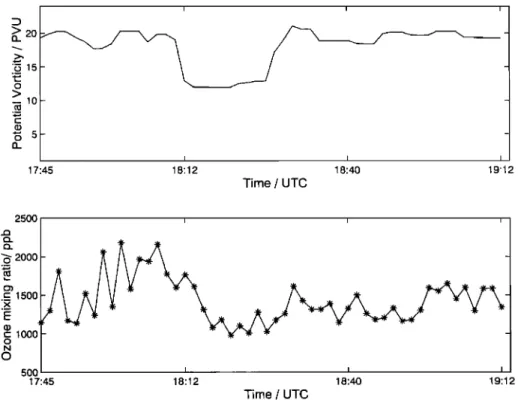
The comparison of the ozone evolution along the flight track with the PV evolution for another polar

filament observed on March 18, 1999, (Figure 2) im-

plies a time shift of 300 s between both data sets that

corresponds to a displacement of about 60 km. Also this flight was performed from Brindisi through a polar filament observed at latitudes relatively far south.

5.2. Subtropical Intrusions

In the case of a subtropical intrusion the lower levels around 380 K are the most interesting ones. On Febru-

ary 29, 1999 the ozone-poor air of the intrusion shows a sharp minimum at 360 K to 380 K. The correlation be-

tween ozone and PV at these levels gives a coefficient of

0.7 at 370 K and 0.5 at 380 K. At 370 K the ozone mini- mum is somewhat more narrow than the one in PV but

located exactly where the minimum in PV occurs. This is reflected in the good correlation. At 380 K the min-

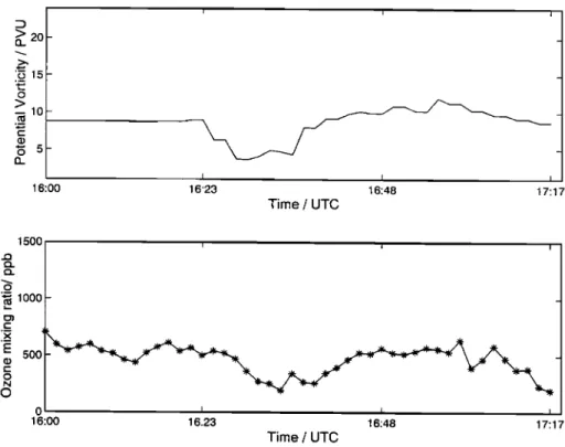
imum in ozone occurs about 500 s later than the min- imum in PV and is somewhat wider (Figure 3). That

means the gradient in ozone is not as sharp as in PV. At 390 K the ozone values are below the detection limit,

and no correlation coefficient could be calculated. At

400 K the correlation of 0.6 is again quite well. Shifting the ozone values 500 s back and recorrelateing the two fields leads to an improvement of the correlation to 0.6

at 380 K and to 0.8 at 400 K. At 370 K the correlation is getting worse (0.3), since the minimum in ozone will

then be misplaced. The improvement of the correla- tion after shifting the ozone field backward in time at

the upper levels of the filament reflects the tilt in the

ozone minimum that has been suggested by the visual

comparison of the ozone anomalies with the PV distri-

bution. The main flight track where the measurements were taken was in direction northeast implying that the upper part of the subtropical intrusion was transported

too slow by the model and placed about 100 km (i.e., 500 s) too far southwest.

•" 20 'G 15 o --10 '• 5- I i I i 1 17:45 18:12 18:40 19:12 Time / UTC

2500

[

,

,

,

-

(•1000

-

Figure 2. (top) Potential vorticity and (bottom) Ozone along the flight track on March 18, 1999

20,020 HEESE ET AL- FORECAST AND SIMULATION OF OZONE FILAMENTS 16:00 _

i

'

'

Figure 3. (top) Potential

vorticity

and (bottom)

Ozone

along

the flight

track

on March

29, 1999

at 380 K.

For another subtropical intrusion observed over Ire-

land on April 6 and 7, 1999 the correlation of the mea-

sured ozone values with the modeled PV distribution

on April 6 could be increased from 0.6 and 0.45 to 0.75 at the levels 380 K and 390 K, respectively, by shifting the PV field 2.5 min of the flight time against the ozone field. On April 7 an improvement of the correlation up

to 0.7 at 370 K and 380 K could be achieved. The shift

of 25 min into direction southeast corresponds to a mis- placement of the subtropical intrusion of about 300 km too far west by the model. This is much more than

found in the other cases, where the displacements of the filaments in PV were in the range of 60 to 100 km.

6. Discussion and Conclusions

Airborne lidar measurements of ozone filaments were

undertaken systematically for the first time during win- ter 1998/1999 using the PV advection model MIMOSA to forecast the occurrence of polar and subtropical air

masses in the midlatitude lower stratosphere. In all

cases the predicted filaments were found in the mea-

sured ozone profiles. To quantify the ability of the model to reproduce the structure and geographical po-

sition of the real filaments, the ozone profiles have been

compared to and correlated with the modeled PV fil-

aments from MIMOSA. Already a visual inspection of

the ozone and PV profiles along the flight track shows

a good agreement between both fields. A correlation

between ozone and PV on the potential temperature levels, where the filaments were observed, deliver coeffi-

cients that reflect a good agreement in the range of the uncertainties of the lidar measurements and the model

input data.

The correlation showed also that the filaments can

sometimes be displaced by the PV advection model. A

shift of about 500 or 300 s has improved the correlation in the case of the polar filaments on February 18 and March 18, respectively. This time shift corresponds to a spatial difference of about 100 and 60 km, or 0.73 ø and

0.5 ø, in both the zonal and the meridional direction. In

case of the subtropical intrusion on March 29, a shift of

about 100 km northeastward, or 0.73 ø, was found in the

upper levels of the ozone minimum. At the lower levels

the position of the intrusion was placed right by the model. On April 6 and 7 the observed displacement is

much larger with about 300 km in direction southeast. This corresponds to 3.3 ø in the zonal and 1.6 ø in the

meridional direction.

Compared to other studies, the displacements found

in the data from the METRO airborne campaign

lie

in the same order of magnitude, except for the last subtropical case on April 6 and 7. For example, New- man and $choeberl [1995] found a correlation of 0.45 be- tween airborne ozone lidar data from the $tratospheric- Tropospheric Exchange project compared to reverse do-

main filling modeled

PV distribution

and a displace-

ment of filament structures less than 1 ø further south

than the ozone

filament.

Flentje et al. [2000]

compared

the ozone data obtained by the Ozone Lidar Experiment lidar on board the German Falcon during the SESAME campaign in winter 1994/1995 with contour advection

HEESE ET AL- FORECAST AND SIMULATION OF OZONE FILAMENTS 20,021

PV odvection model MIMOSA on 29.03.1999 ot level 580K

12.0 1 1.0 10.0 9.0 8.0 7.0 6.0 5.0 4.0 5.0 2.0 1.0 0.0 Flight trock 45O

Lidar

O3-profiles

from

METRO-flight

on

29/03/1999

f 1400 44O 430 420 "• 410 E 400 = 390 o 380 370 36O 350 ' * ' 16:00 16:23 16:50 17:17 Time / UTC 1200 1000 8OO O N O 600 •3 400 200 JO

Plate 3. (top)

Modeled

PV distribution

at 380

K on March

29, 1999

at 1600

UTC.

Measurements

during

this

round

flight

startet

at point

a and

ended

at point

b. (bottom)

Measured

ozone

profiles

20,022 HEESE ET AL.- FORECAST AND SIMULATION OF OZONE FILAMENTS

PV advection model MIMOSA cross-section on 29.03.1999

4,50 440 450 420 410 400 590 ,5.1 580 6.5 570 560 5,50 16:00 , / 16:25 16:47 Time / UTC 9.0 8.1 7.2 4.5 "' 5.6 2.7 17:17 45O 440 43O 420 410 400 390 380 370 360 350 16:00

Lidar

03-profiles

from

METRO-flight

on 29/03/1999

i I ., 16:23 16:50 17:17 Time / UTC lOO 80 60 40 20 0 i o • o -20 • -40 -60 -80 -lOO

Plate 4. (top) Modified PV cross

section

during flight on March 29, 1999. The dashed

line

indicates the level 380 K shown on the horizontal map in Plate 3. (bottom) Ozone anomalies calculated with respect to the mean ozone profile for this flight.

HEESE ET AL.: FORECAST AND SIMULA•rION OF OZONE FILAMENTS 20,025

PV cross sections and found a meridional displacement

of less than 0.5 ø in 70% of the cases, and 10% showed a displacement of more than 1 ø.

A major part of the displacements of the filaments found in the METRO study can be explained by the uncertainties of the input data to the model MIMOSA.

A mean error in ECMWF (31 and 50 level version)

wind velocity of 2.5 ms

-1 in the region between

30

and 70 hPa (around 20 km altitude) was found compar-

ing the ECMWF analysis wind vectors to the velocities

measured during long-duration balloon flights [Knud- sen et al., 1999]. This error leads to a displacement of

7 ø after 10 days in trajectory calculations. Since the polar filaments observed at 435 K correspond to an al-

titude around 17 to 18 km, we can assume an error in

ECMWF winds of the same magnitude. For the sub-

tropical intrusions at levels around 380 K the error may

differ. The displacements observed in MIMOSA for po-

lar filaments at levels around 435 K are much smaller

than the ones found for trajectory calculations. Even in the last subtropical case on April 6 and 7 the displace- ment is only about half the displacement found for the

trajectory calculations. This is evident since the errors

of the position of the filaments depend less on the wind velocity in the direction of the trajectories but more on

the error perpedicular to the direction of the trajecto-

ries.

The sensitivity to errors in the wind data of the PV

advection model MIMOSA has been estimated for a fil-

ament observed in December 1997, (Hauchecorne et al.,

submitted manuscript, 2001). Two types of errors were

assumed:

(1) a constant

error of 1 ms

-• in direction

of

the wind, and (2) a constant

error of 0.2 ms

-• perpen-

dicular to the direction of the wind. After 10 days of

advection the mean error of the position of a filament, perpendicular and parallel to the filament, has been es-

timated: For the first case

(1 ms

-•) the error for the

position of the filament was 95 km perpendicular and

295 km parallel to the filament. For the second case

(0.2 ms

-•) the error was 80 km perpendicular

to the

filament and 160 km parallel to the filament. These er-

rors compare quite well to the displacements of 60 km and 100 km perpendicular to the filaments found for three of the METRO flights. Regarding the large dis- placements found for the second subtropical intrusion, a review of the ECMWF wind velocities during the 10 days of advection used in the model showed that the

circulation at 380 K in the end of the winter is much

more disturbed and errors in the input wind data may be higher.

Finally, we can state that the modeled and observed

structures in the PV and ozone fields are of comparable

size. Air masses of polar, midlatitude, and subtropi-

cal origin were well distinguished by the modeled PV gradients. The position of the filaments could be sim-

ulated with small displacements in most cases of 0.5 ø

to 0.7 ø .

in this study can be accounted for by the estimated er-

ror in the ECMWF wind fields. The model was used

to forecast the filaments and to plan the flights during the METRO campaign, and the predicted polar fila- ments and subtropical intrusions were always detected

by the ozone lidar measurements. Thus the PV advec-

tion model MIMOSA is suitable for studies of the merid-

ional transport of polar and subtropical air masses into midlatitudes. A study of the influence of the filamenta-

tion processes on the ozone amount will be undertaken

including the lidar and ozone sonde measurements of the ground-based station at the Observatoire de Haute

Provence (S. Godin et al., Influence of the Artic polar

vortex erosion on the lower stratospheric ozone amounts

at OHP (44øN, 6øE), submitted to J. Geophys. Res., 2001). Furthermore, MIMOSA has been used to eval-

uate the transport of air across the polar vortex edge

during the four last winters (Hauchecorne et al., sub- mitted manuscript, 2001).

For further studies, the model was coupled with the chemical part of the French chemical transport model

REPROBUS [Lefevre et al., 1994] to account for the ozone destruction observed in other winters. Observa-

tions show very high local ozone loss of over 60% during

winter 1999/2000 inside the Arctic polar vortex. Fortu-

nately, the METRO campaign could be extended into winter 2000 in the framework of the European project

THESEO 2000, and additional airborne lidar measure-

ments of polar filaments became feasible. Although the

stable polar vortex kept the polar air inside its bound-

aries most of the time, several flights through polar fil-

aments could be performed. These data are still under

investigation and will be analyzed using the coupled

MIMOSA-REPROBUS model IMarchand et al., 2000]

together with the measurements from the ground-based

network.

Acknowledgments. We are grateful to G. Ancellet to provide the ALTO lidar and would like to thank the staff

at Institute Oeographique National (ION) for the logistics

and the performances of the flights. We will also thank our colleagues at Institute National de Science de l'Univers

(INSU) who have processed the accompanying flight data.

Many thanks to Bernard Legras and his group who pro- vided the PV calculation scheme. Finally, we want to thank Jean Louis Conrad, Anne (•arnier, Christian Laqui, Claude

Leroy, Jean-Pierre Marcovici, and Jacques Porteneuve for

their help concerning the lidar system and data aquisition.

Thanks to the suggestions of two anonymous reviewers. Due to their comments the paper has been substantially im-

proved. This work was funded by the European commis-

sion through the project THESEO- METRO under contract ENV4-CT97-0529.

References

Ancellet, G., and F. Ravetta, Compact airborne lidar for tropospheric ozone: Description and field measurements,

Appl. Opt., S'7, 5509-5521, 1998.

Butchart, N., and E. E. Remsberg, The area of the strato-

20,024 HEESE ET AL.: FORECAST AND SIMULATION OF OZONE FILAMENTS

on an isentropic surface, J. Atmos. $ci., •3, 1319-1339,

1986.

de Schoulepnikoff, L., V. Mitev, V. Simeonov, B. Calpini, and H. van den Berg, Experimental investigation of high- power single-pass Raman shifters in the ultraviolet with

Nd:YAG and KrF lasers, Appl. Opt., 36, 5026-5043, 1997.

Flentje, H., W. Renger, M. Wirth, and W. A. Lahoz, Val-

idation of contour advection simulations with airborne

Lidar measurements of filaments during the second Eu-

ropean Stratospheric Arctic and Midlatitude Experiment

(SESAME), J. Geophys. Res., 105, 15,417-15,437, 2000.

Holton, J. R., P. H. Haynes, M. E. Mcintyre, A. R. Douglas,

R. B. Rood, and L. Pfister, Stratosphere-troposphere ex-

change, Rev. Geophys., 33,403-439, 1995.

Hood, L., S. Rossi, and M. Beulen, Trends in lower strato-

spheric zonal winds, Rossby wave breaking behavior, and

c•lumn ozone at northern midlatitudes, J. Geophys. Res., 10•, 24,321-24,339, 1999.

Knudsen, B. M., J.P. Pommereau, A. Garnier, M. Numez- Pinharanda, L. Denis, F. Nouel, V. Duborg, and G. Le- trenne, Comparison of calculated trajectories with long

duration balloon data, paper presented at 5th European

Workshop on Stratospheric Ozone, European Commis- sion, Saint-Jean-de-Luz, France, Sept. 27- Oct. 1, 1999. Lait, L. R., An alternative form for potential vorticity, J.

Atmos. Sci., 51, 1754-1759, 1996.

Lefevre, F., G. B. Brassuer, I. Folkins, A. K. Smith, and P.

Simon, Chemistry of the 1991-1992 stratospheric winter: Three-dimensional model simulations, J. Geophys. Res., 99, 8183-8195, 1994.

Marchand, M., S. Godin, B. Heese, and A. Hauchecorne, A study of polar filaments using the coupled model MIMOSA-REPROBUS, paper presented at Quadrennial Ozone Symposium, EORC•NASDA, Sapporo, Japan,

July 3- 8, 2000.

Naujokat, B., The winters 1997/98 and 1998/99 in per- spective, paper presented at 5th European Workshop on Stratospheric Ozone, European Commission, Saint-Jean- de-Luz, France, Sept. 27- Oct. 1, 1999.

Newman, P. A., and M. R. Schoeberl, A reinterpretation

of the data from the NASA stratosphere-troposphere ex-

change project, Geophys. Res. Lett., 22, 2501-2504, 1995. Norton, W. A., and M.P. Chipperfield, Quantification of the transport of chemically activated air from the northern hemispheric polar vortex, J. Geophys. Res., 100, 25,817-

25,840, 1995.

Orsolini, Y., D. Cariolle, and M. Deque, Ridge formation in

the lower stratosphere and its influence on ozone trans-

port: A general circulation model study during late Jan- uary 1992, J. Geophys. Res., 100, 11,113-11,135, 1995. Papayannis, A.D., G. N. Tsikrikas, and A. A. Serafetinides,

Generation of UV and VIS laser light by stimulated Ra-

man scattering in H9., D9./He using a pulsed Nd:YAG laser

at 355 nm, Appl. Phys. B, 67, 1-7, 1998.

Reid, S. J., and G. Vaughan, Lamination in ozone profiles in the lower stratosphere, Q. J. R. Meteorol. Soc., 117,

825-844, 1991.

Reid, S. J., G. Vaughan, and E. Kyro, Occurrence of ozone laminae near the boundary of the stratospheric polar vor-

tex, J. Geophys. Res., 98, 8883-8890, 1993.

Vaughan G., and C. Timmis, Transport of near-tropopause

air into the lower midlatitude stratosphere, Q. J. R. Me- teorol. $oc., 12•, 1559-1578, 1998.

World Meteorological Organization, Scientific Assessment of Ozone Depletion: 1998, in Global Ozone Research and Monitoring Project, Rep. 1•, Geneva, 1998.

B. Heese, Meteorological Institute, University of Munich, Theresienstr. 37, D-80333 Munich, Germany.

(b.heese@gtco.de)

S. Godin, Service d'Aeronomie du CNRS, Universite Pierre et Marie Curie, 4, Place Jussieu, Boite 102, F-75252 Paris Cedex 05, France.

(sophie.godin@aero.j ussieu.fr )

A. Hauchecorne, Service d'Aeronomie du CNRS, BP3,

F-91371 Vcrrieres-le-Buisson Cedex, France.

( alain. hauchecorne@aerov.j ussieu. fr )

(Received April 14, 2000; revised October 2, 2000; accepted November 21, 2000.)