HAL Id: hal-01586016
https://hal.archives-ouvertes.fr/hal-01586016
Submitted on 12 Sep 2017
HAL is a multi-disciplinary open access archive for the deposit and dissemination of sci-entific research documents, whether they are pub-lished or not. The documents may come from teaching and research institutions in France or abroad, or from public or private research centers.
L’archive ouverte pluridisciplinaire HAL, est destinée au dépôt et à la diffusion de documents scientifiques de niveau recherche, publiés ou non, émanant des établissements d’enseignement et de recherche français ou étrangers, des laboratoires publics ou privés.
Bayesian multiproxy temperature reconstruction with
black spruce ring widths and stable isotopes from the
northern Quebec taiga
Fabio Gennaretti, Huard David, Naulier Maud, Martine M. Savard, Christian
Begin, Dominique Arseneault, Joel Guiot
To cite this version:
Fabio Gennaretti, Huard David, Naulier Maud, Martine M. Savard, Christian Begin, et al.. Bayesian multiproxy temperature reconstruction with black spruce ring widths and stable isotopes from the northern Quebec taiga. Climate Dynamics, Springer Verlag, 2017, �10.1007/s00382-017-3565-5�. �hal-01586016�
Bayesian multiproxy temperature reconstruction with black
spruce ring widths and stable isotopes from the northern Quebec
taiga
Fabio Gennaretti1 · David Huard2 · Maud Naulier3 · Martine Savard4 · Christian Bégin4 · Dominique Arseneault5 · Joel Guiot1
Received: 21 July 2016 / Accepted: 31 January 2017
© The Author(s) 2017. This article is published with open access at Springerlink.com
Ring width showed a larger response to single eruptions and a larger cumulative impact of multiple eruptions dur-ing active volcanic periods, δ18O showed intermediate responses, and δ13C was mostly insensitive to volcanic eruptions. We conclude that all reconstructions based on a single proxy can be misleading because of the possible reduced or amplified responses to specific forcing agents.
Keywords Tree-ring · Oxygen isotopes · Carbon
isotopes · Last millennium · Summer temperature · Volcanic impact · Proxy sensitivity
1 Introduction
In North America, the network of proxy records used for high-resolution climate reconstructions over the last two millennia is dominated by tree-ring chronologies. How-ever, these chronologies are much more abundant in the
Abstract Northeastern North America has very few
millennium-long, high-resolution climate proxy records. However, very recently, a new tree-ring dataset suitable for temperature reconstructions over the last millennium was developed in the northern Quebec taiga. This data-set is composed of one δ18O and six ring width chronolo-gies. Until now, these chronologies have only been used in independent temperature reconstructions (from δ18O or ring width) showing some differences. Here, we added to the dataset a δ13C chronology and developed a signifi-cantly improved millennium-long multiproxy reconstruc-tion (997–2006 CE) accounting for uncertainties with a Bayesian approach that evaluates the likelihood of each proxy model. We also undertook a methodological sen-sitivity analysis to assess the different responses of each proxy to abrupt forcings such as strong volcanic eruptions.
Electronic supplementary material The online version of this
article (doi:10.1007/s00382-017-3565-5) contains supplementary
material, which is available to authorized users. * Fabio Gennaretti [email protected] David Huard [email protected] Maud Naulier [email protected] Martine Savard [email protected] Christian Bégin [email protected] Dominique Arseneault [email protected] Joel Guiot [email protected]
1 Aix Marseille Univ, CNRS, IRD, Coll France, CEREGE,
13545 Aix-en-Provence, France
2 Ouranos Consortium, 550 Rue Sherbrooke O,
H3A1B9 Montréal, Canada
3 Institut de Radioprotection et de Sûreté Nucléaire, CEA
Cadarache, 13108 Saint-Paul-Lez-Durance, France
4 Geological Survey of Canada, Natural Resources Canada,
490 Rue de la Couronne, G1K9A9 Québec, Canada
5 Département de biologie, chimie et géographie, Université
du Québec à Rimouski, 300 allée des Ursulines, G5L3A1 Rimouski, Canada
west than in the east and, importantly, there are only five chronologies spanning more than a millennium north of the 50th parallel (Pages 2k Consortium 2013; http://past-globalchanges.org/ini/wg/2k-network/intro). In northeast-ern North America, developing tree-ring chronologies is highly challenging due to short tree longevity, the high frequency and severity of wildfires and the remoteness of many areas (Arseneault et al. 2013). To improve the qual-ity of reconstructions in such regions with scarce proxy data, we can both increase series replication for a single proxy by creating new chronologies, and combine prox-ies with an independent response to climate forcing. In this paper, we adopted the solution of combining proxies using datasets from the northern Quebec taiga. Six highly replicated millennium-long ring width chronologies were recently developed in this region by Gennaretti et al. (2014) with black spruce [Picea mariana (Mill.) B.S.P] subfos-sil trees preserved in six lakes. Samples from one of these sites were also used to obtain a millennium-long record of oxygen isotopic ratios (δ18O) in tree-ring cellulose (Naulier et al. 2015). Until now, these ring width and δ18O data have only been used separately in independent summer tempera-ture reconstructions. In principle, merging these data in a multiproxy approach should provide more robust estimates of the past regional climate variations. Indeed, within a multiproxy framework, we can exploit the distinct climatic responses embedded in each proxy to reduce the impact of individual proxy errors.
Multiproxy approaches at the regional scale have already been used with successful results (Sidorova et al. 2012,
2013). For example, McCarroll et al. (2013) improved their temperature reconstruction by combining chronologies of ring width, ring density and annual tree height growth from Scandinavian sites. Boucher et al. (2011) reconstructed the full spectra of a drought index in southern South America using only the reliable periodicities specific to each of their proxies. Tolwinski-Ward et al. (2015) improved their local temperature-soil moisture reconstructions using both ring width and isotopic data within a hierarchical Bayes-ian approach, allowing a better understanding of the tem-poral changes in the climatic controls on the proxies. Such Bayesian methods are especially useful for leveraging the multi-proxy information and for assessing uncertainties with a probabilistic perspective. Bayesian models have thus been used to (1) improve climate field reconstructions from multi-proxy networks (Tingley and Huybers 2010), (2) bet-ter infer climate variability from nonlinear proxies (Emile-Geay and Tingley 2016), (3) define spatially varying proxy-climate relationships (Tierney and Tingley 2014) or (4) investigate the mechanistic climate controls on the proxies (Tolwinski-Ward et al. 2013).
In this study, we present a new millennium-long δ13C chronology in tree-ring cellulose, which enhances the
temperature-sensitive proxy dataset from the northern Que-bec taiga. Thus, we use an ensemble of three proxies (ring width, δ18O and δ13C) to provide the first multiproxy regional high-resolution summer temperature reconstruction in north-eastern North America over the last millennium (997–2006 CE). A linear Bayesian approach is used to generate sharp and reliable confidence intervals based on the likelihood and the convergence of the proxy models. Finally, the sensitivity of individual proxies to temperature perturbations is evalu-ated and discussed, focusing the analysis on the response to strong volcanic eruptions because they produce abrupt per-turbations after key-dates.
2 Materials and methods 2.1 Proxy and climate data
The tree-ring data from the northern Quebec taiga are com-posed of six millennium-long ring width chronologies devel-oped with series from 1782 subfossil stem segments and 150 living black spruces (Gennaretti et al. 2014). Subfossil logs were sampled from the water and sediments of the littoral zone of six boreal lakes (the coordinates of the central point are 54.23 N and 71.39 W), while living trees were selected in the lakeshore forest of the same sites. Their cross-sections are stored at the University of Quebec in Rimouski, and the series are already in the public domain (http://www.ncdc.noaa.gov/ paleo). Here, we used the median of the 6 millennium-long site-specific chronologies keeping for each site only periods with sample depth greater than five. Individual chronolo-gies were built with the regional curve standardization (RCS) pivot correction method to reduce the impact of varying sam-pling heights (Autin et al. 2015). Low and high frequencies of the median chronology were treated separately. Low fre-quencies (LFs) were obtained with a 9-year triangular filter to produce a chronology comparable to that of the stable iso-topes (see below). High frequencies (HFs) were obtained by subtracting the LFs from the raw chronology. The bandwidth of the LF filter at the 50% threshold was 0.07 cycles/year. The LF chronology was also transformed to obtain a quasi-perfect Gaussian distribution with the inverse transform sampling technique. This technique is based on a quantile-based trans-formation and, in some cases, should improve the linearity of the relationship between proxies and normally distributed climate variables (Emile-Geay and Tingley 2016; van Albada and Robinson 2007):
where erf represents the Gauss error function, P(y) the proxy cumulative distribution function and yi and y′i the
proxy untransformed and transformed values, respectively, for year i. Fig. S1 (see electronic supplementary material) (1)
shows the effect (quite low in this case) of this transforma-tion on the LF chronology.
From one of the six sites from the northern Quebec taiga, 60 subfossil logs and 5 living trees were further ana-lyzed at the Delta-lab of the Geological Survey of Canada to extract two millennium-long chronologies of stable iso-tope ratios in tree-ring cellulose. The δ18O chronology is already in the public domain (Naulier et al. 2015), whereas the δ13C chronology is detailed here and is accessible in the supplementary material (Dataset S1). These chro-nologies were built with the “offset-pool plus join-point” method (Gagen et al. 2012) to obtain an annual resolution from five tree replicates (this replication was proven to be adequate to obtain robust site chronologies; Naulier et al.
2014) and successive tree cohorts. Assuming that the five time series of each cohort are realizations of the same sto-chastic process, this method produces chronologies equiva-lent to time series smoothed by the aforementioned 9-year triangular filter. Indeed, within every cohort of five trees, the rings of each tree were divided into 5-year blocks for the isotopic measurements with an offset of 1 year among trees (Naulier et al. 2015). The δ13C values of the modern part of the chronology were also mathematically corrected for atmospheric δ13C CO
2 changes due to fossil fuel com-bustion (Suess effect), and for plant response to increasing
isotopes. The relationships between the temperature vari-able and the proxies over the last century are shown in Fig. S4.
2.2 Bayesian proxy analysis
Our objective was to infer the values of the mean July–August temperature for each year over a past period where the temperature is unknown. This inference was based on a set of known proxy values (D) and temperature observations (T) that overlap over a calibration period (cal; 1905–2006). Using Bayes’ theorem, the posterior distribu-tion of temperature t at each year i can be obtained by:
In Eq. (2), the first term in the numerator is the proxy likelihood, the second term of the numerator is the prior distribution for temperature, and the denominator is a nor-malization constant. If we assume that a model exists that estimates the proxy value given the July–August tempera-ture and a vector of hyperparameters (𝜏), then the proxy likelihood can be written as:
(2)
p(ti|Di, Dcal, Tcal)= p
(
Di|ti, Dcal, Tcal)p(ti|Tcal, Dcal)
p(Di|Tcal,Dcal) .
atmospheric CO2 concentrations (McCarroll et al. 2009; McCarroll and Loader 2004; Naulier et al. 2014). The final isotope ratio chronologies are compared with the ring width LF chronology in Fig. S2. As with the ring width chronol-ogy, the isotope chronologies were also transformed with the inverse transform sampling technique (Fig. S1).
The monthly climate data for our study area (1901–2010) were downloaded from the Climatic Research Unit (CRU) TS 3.23 climate dataset (Harris et al. 2014). A correlation analysis showed that the mean of the July and August tem-perature was the common best fit climate signal registered by our proxies (Fig. S3). Thus, this variable was retained for the climate reconstruction. This is consistent with previ-ous findings showing that summer temperatures control the growth and isotopic values of these trees (Gennaretti et al.
2014; Naulier et al. 2014, 2015). Low and high tempera-ture frequencies were treated separately and obtained with the same method as for the ring width chronology such that the LF chronology was comparable with that of the stable
(3)
p(Di|ti, Dcal, Tcal)= ∫ p(Di, 𝜏|ti,Dcal.Tcal)d𝜏
= ∫ p(Di, Dcal|𝜏, ti,Tcal)p(𝜏|ti, Tcal
)
∕p(Dcal| ti,Tcal)d𝜏
∝ ∫ p(Di|ti, 𝜏)p(Dcal|Tcal, 𝜏)p(𝜏)d𝜏.
On the second line, the denominator term p(Dcal| ti,Tcal)
appearing through the second application of Bayes theorem is again assumed constant. The third line includes, from left to right, the likelihood of the proxy datum Di, the likelihood
of the calibration data Dcal, and the prior over-the-proxy
model hyperparameters. In a sense, both the model calibra-tion and the model prediccalibra-tion were merged into one formula. The posterior can be solved by making assumptions about the likelihoods and the priors. Here, we assume that the prior over July–August temperature ti is a normal
dis-tribution for which parameters are given by the moments of the previous STREC reconstruction (Summer Tempera-ture Reconstruction for Eastern Canada) based only on ring width series (Gennaretti et al. 2014):
Next, considering that we did not find evidence of non-linearity in the proxy-climate relationships, the model for computing the proxy likelihood can be defined by a linear regression with normally distributed errors:
(4)
A prior for the used hyperparameters (𝜏) also needs to be defined, and here, we chose non-informative priors for sim-plicity (Fig. S5): a uniform prior for the intercept, a Jeffreys prior for the variance and a prior for the slope that respects the invariance over the choice of dependent and independ-ent variables (i.e., uniform prior in sin(tan− 1α)). We thus obtained the following minimally informative prior on the models:
The last step is to substitute the generic data Dwith our three proxy datasets (R for ring width, O for δ18O and C for δ13C) and to introduce a set of hyperparame-ters specific to each proxy, denoted by 𝜏R, 𝜏O, 𝜏C.We can
now write the posterior of Eq. (2) as:
In practice, Eq. (7) is solved using Markov Chain Monte Carlo (MCMC) sampling with Metropolis–Hast-ings steps. Instead of sampling all 10 dimensions (three hyperparameter vectors plus ti) at once, each hyperpa-rameter vector is sampled independently according to
p(Dcal|Tcal, 𝜏)p(𝜏) (Fig. S5). The samples are then used independently to obtain a temperature posterior distribu-tion from each proxy or all together to obtain a sharper distribution using the proxy ensemble (Figs. S6, S7). The spread of the distribution of each of the proxy mod-els is an indication of the weight (confidence) of each proxy.
To account for the fact that isotopic series were smoothed in the measurement process and their HFs were lost, the temperature LFs (tlow) were reconstructed with
the three proxies (ring width, δ18O and δ13C), whereas the temperature HFs (thigh) were reconstructed with ring
widths only. The LF and HF components are independ-ent, each described by a model with its set of hyperpa-rameters (Fig. S5). The posterior distributions of tlow
and thigh for each year i were then combined in the final
reconstruction.
The posterior probability of models with different combinations of LF proxies was also evaluated with the following equation (Kruschke 2014):
(5) p(Di|ti, 𝜏 ) ≡ N(Di; 𝜇= 𝛼ti+ 𝛽, 𝜎 ) , 𝜏≡ (𝜇, 𝛼, 𝜎). (6) p(𝜏) ≡ p(𝛼, 𝛽, 𝜎) ∝ (1 + 𝛼 2)(−3∕2) 𝜎 . (7)
p(ti|Ri, Rcal, Oi, Ocal, Ci, Ccal, Tcal
) ∝ ∫ p(Ri|ti, 𝜏R ) p(Rcal|Tcal, 𝜏R ) p(𝜏R ) d𝜏R × ∫ p(Oi|ti, 𝜏O)p(Ocal|Tcal, 𝜏O)p(𝜏O)d𝜏O × ∫ p(Ci|ti, 𝜏C ) p(Ccal|Tcal, 𝜏C ) p(𝜏C ) d𝜏Cp(ti). (8) p�m� Tcal,Dcal � = p � Tcal� m, Dcal�p(m) ∑7 m=1p � Tcal� m, Dcal�p(m) .
In Eq. (8), m is an indexal parameter specific to each of the 7 possible combinations of proxies (R, O, C, R&O, R&C, O&C, R&O&C), p(m| Tcal,Dcal)
is the posterior probability of the proxy model,
p(Tcal| m, Dcal) is the likelihood of the data given the
model, and p(m) is the prior probability of the model. Equation (8) is solved considering uniform model prior probabilities (p(m) = 1∕7), and evaluating the likelihood of the temperature calibration data with
p(Tcal|m, Dcal)= ∫ p(Tcal|m, Dcal, 𝜏m)p(𝜏m)d𝜏m. To be
clear, if m = 4 and the proxy considered are R and O, then
p(Tcal|m = 4, Dcal ) = ∫ p ( Tcal|Rcal, 𝜏R ) p(𝜏R ) d𝜏Rp ( Tcal| Ocal, 𝜏O)p(𝜏O ) d𝜏O.
2.3 Impact of uncertainties in the proxy chronologies
The proposed Bayesian model evaluates the capacity of the proxies to reconstruct temperature values based on
the relationship over the calibration period and consid-ers uncertainties in model parameter estimation. There is no source of uncertainty that depends on time in the model. However, we implicitly evaluated the impact of the time-varying uncertainties in the LF proxy chronol-ogies, which depend on the spread of individual series. All the used proxy chronologies are built with an almost stable sample depth over the last millennium. For each year we computed the probability density of the proxy chronology values assuming that the available replicates (three to six site-specific chronologies for ring width and cohorts of five trees for isotopes) are normally distributed (Fig. S8). These probability densities were sampled 100 times to create 100 chronologies per proxy to be included in the Bayesian model. The spread of the resultant 100 temperature reconstructions represent the impact of the uncertainties in the proxy chronologies.
3 Results and discussion 3.1 Final reconstruction
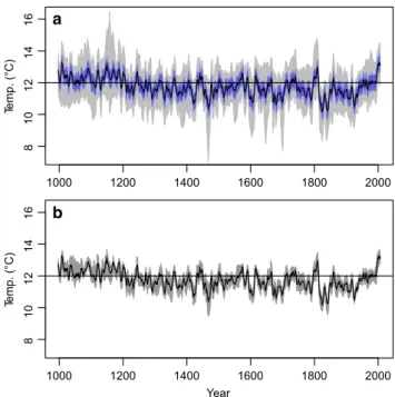
The final reconstruction (Three Proxies Summer Tem-perature Reconstruction for Eastern Canada, here-after 3P-STREC) and its confidence intervals were derived from the median, 5th and 95th percentiles of
the temperature posterior densities of each year (Fig. 1). The R2 of the LF 3P-STREC versus the temperature of the last century was 0.81. This is a substantial improve-ment relative to previous reconstructions with the same ring width data (STREC; R2 = 0.64; Gennaretti et al.
2014) or with the same δ18O data (i-STREC; R2 = 0.58 or 0.64 if considering mean maximal temperature values such as in Naulier et al. 2015). Note that here and hereaf-ter, the comparisons with previous data were performed
under the same conditions (using the same climate vari-able, frequency components, smoothing algorithm and 1905–2006 or 997–2006 periods). The added value of the multiproxy approach is clearly shown in Fig. 2. The posterior probability of the model with the three proxies was higher than the probability obtained with any other combination of one or two proxies. The Bayesian frame-work also allows sharp and reliable confidence intervals to be produced by leveraging the multiproxy information. Indeed, 95.1% of the observed temperature values were inside the 90% 3P-STREC nominal confidence inter-vals despite the spread of the 3P-STREC temperature posterior distributions being only 39% of the overall spread of the distributions obtained using the three prox-ies independently (Fig. 3a). The Bayesian model per-formed satisfactorily also over independent validation periods when the full period with temperature observa-tions (1905–2006) was spit for a cross-calibration vali-dation exercise (Table S1). The confidence intervals of 3P-STREC did not increase back in time because there is no source of uncertainty that depends on time in the model. However, the confidence intervals did not signif-icantly vary even when we evaluated the impact of the Year 1800 1850 1900 1950 2000 81 01 21 41 6 Te mp. (°C ) b 1000 1200 1400 1600 1800 2000 81 01 21 41 6 Te mp. (°C) a
Fig. 1 The entire 3P-STREC reconstruction (a; 997–2006) and a
zoom over the last two centuries (b; 1800–2006) with low frequen-cies only (black bold lines) and with high frequenfrequen-cies added (black thin lines). The 90% confidence intervals are also shown (dark blue for the low frequency reconstruction and light blue for the final recon-struction). Red lines are mean July–August temperature values (CRU TS3.23; low frequencies only with bold lines and low plus high fre-quencies with thin lines)
Proxy combination
Model poste
rior probabilit
y
C R O R_C O_C R_O R_O_C
0.00
0.05
0.10
0.15
Fig. 2 Posterior probability of models with different combinations
of low frequency proxies. The models are ordered according to their
probability. R for ring width, O for δ18O and C for δ13C
1000 1200 1400 1600 1800 2000 81 01 21 41 6 Te mp. (°C) Year b 1000 1200 1400 1600 1800 2000 81 01 21 41 6 Te mp. (°C) a
Fig. 3 Evaluation of uncertainties. a Reduction of
reconstruc-tion uncertainties with the proposed Bayesian methodology, which exploits the convergence of the three proxies. The figure shows the 90% confidence intervals of the low frequency 3P-STREC recon-struction (blue) and those derived from the sum of three independ-ent temperature posterior densities for each year obtained from single proxies (light gray). b 90% confidence intervals of the reconstruction when considering an independent time-varying source of uncertainty due to individual series spread in each low frequency proxy chronol-ogy (dark gray)
time-varying uncertainties in the LF proxy chronologies (Fig. 3b). This is because the sample depths of the used chronologies were quite stable.
When the HFs (reconstructed with ring width only) were added to the LF 3P-STREC (Fig. 1), the R2 of the final reconstruction versus the temperature of the last century was 0.41. Again, this is a notable improvement over STREC (R2 = 0.30). This improvement mostly reflects the more realistic decadal and longer term signals achieved with the multiproxy approach. Indeed, HFs in 3P-STREC did not improve because they were only based on ring width data (R2 = 0.11 with HF July–August tem-perature values; Fig. S4) and were very similar to those of STREC. A coherency plot (Fig. S9) also showed that the fidelity of 3P-STREC is especially strong at medium (frequency = 0.33 corresponding to 3 year periodicities) and low frequencies (frequency < 0.1 corresponding to decadal and longer time-scales). For the final 3P-STREC, 92.16% of the observed temperature values were within the 90% nominal confidence intervals. However, the inter-annual variability was underestimated because ring width HFs have a low predictive power. The develop-ment of wood density chronologies has the potential to improve the HF results.
The previous reconstructions with the same data (STREC from ring width and i-STREC from δ18O) have suggested that the Medieval Climate Anomaly (MCA) was particularly warm in the Quebec taiga (Fig. 4a, b). The LF 3P-STREC confirmed this result, but it also sug-gested that the 15-year period between 1992 and 2006 was the warmest of the last millennium (Table S2). However, when HFs were added, some years during the Middle Ages and even during the Little Ice Age (LIA, 1300–1850) became as warm as the last decade (Fig. 1; Table S2). In addition, considering that the inter-annual variability of the final 3P-STREC was underestimated, more extreme warm years have probably occurred in the past. These findings are consistent with the fact that the MCA and the LIA were not necessarily synchro-nous everywhere in the World, and their intensity also varied spatially (Luterbacher et al. 2016; Mann et al.
2009). These spatial variations could be explained by regional climate feedbacks, such as those related to the Greenland sea ice and Labrador current dynamics in the case of the Quebec–Labrador peninsula (Miller et al.
2012; Schleussner and Feulner 2013; Stenchikov et al.
2009; Zanchettin et al. 2012; Zhong et al. 2011). The 3P-STREC reconstruction also allowed a better definition of the cold periods during the LIA in the Quebec taiga. According to i-STREC (Naulier et al. 2015), the coldest period in this region was between 1660 and 1700 during the Maunder solar minimum, while according to STREC (Gennaretti et al. 2014), the coldest period was between
1000 1200 1400 1600 1800 2000 −4 −2 024 Year Inde x d 1000 1200 1400 1600 1800 2000 −4 −2 02 4 Inde x c 1000 1200 1400 1600 1800 2000 −3 −2 −1 01 23 Inde x b 1000 1200 1400 1600 1800 2000 −3 −2 −1 01 2 3 Inde x a
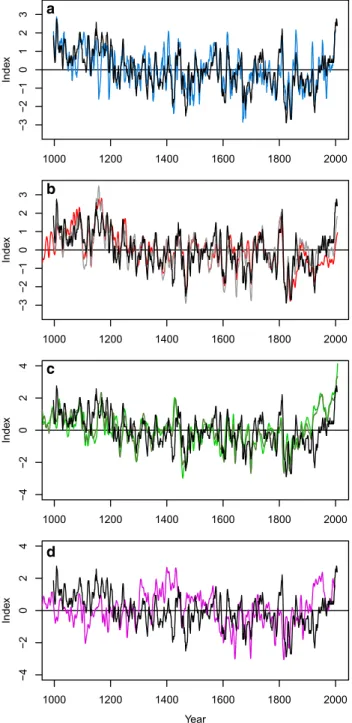
Fig. 4 Comparison with previous and other up-to-date
reconstruc-tions. a Low frequency 3P-STREC (black) compared with i-STREC
(blue, Naulier et al. 2015, reconstruction using oxygen isotopes only).
b Comparison with STREC (red, Gennaretti et al. 2014, reconstruc-tion using ring width only) and a STREC variant (gray) where the chronologies are built with the pivot correction RCS method (Autin
et al. 2015). c Comparison with N-TREND summer temperature
reconstruction (dark green; Wilson et al. 2016) based on 54 Northern
Hemisphere tree-ring records including our ring width record. The median of all records in N-TREND excluding ours is shown in light green. d Comparison with the Northern Hemisphere mid-latitude temperature reconstruction based on 15 maximum latewood density
chronologies (violet; Schneider et al. 2015). All plotted series are
1810 and 1860 coinciding with a part of the Dalton mini-mum and some active volcanic decades. The 3P-STREC reconstruction supported this second alternative that the first half of the nineteenth century was likely the cold-est period of the LIA and of the last millennium in the Quebec taiga (Fig. 1). Another improvement achieved with the new Bayesian multiproxy reconstruction, was to confirm a more realistic long-term cooling trend over the last millennium (−0.75 ± 0.07 °C per 1000 years; esti-mate ± SE; computed on the final 3P-STREC). This trend, probably due to a combination of orbital changes (Kauf-man et al. 2009; Esper et al. 2012) and volcanic activ-ity (Miller et al. 2012), is more similar to that previously reconstructed with the same δ18O data (−0.52 ± 0.04 °C per 1000 years; i-STREC) than with the same ring width data (−1.60 ± 0.11 °C per 1000 years; STREC) and is quite consistent with values already published for nearby regions (Miller et al. 2013; Viau et al. 2012).
The concordance of 3P-STREC with the recent N-TREND Northern Hemisphere summer temperature reconstruction based on tree-ring width and density records (Wilson et al. 2016) is impressive if we exclude the last century (Fig. 4c), despite the very different spatial domain of these two reconstructions (a similar conclusion can also be drawn if the comparison is done with the reconstruction of Stoffel et al. 2015, as shown in Fig. S10). It has been suggested that few robust tree-ring chronologies along the northern North-Hemisphere treeline are sufficient to pro-duce good estimates of reconstructions obtained with much larger networks of tree-ring data (D’arrigo and Jacoby
1993). Our study further suggests that a single regional reconstruction (maximum distance between sampling sites is 150 km), extremely well replicated at the site and the tree levels (six homogeneous sites and measurements from 1932 trees), may be very similar to an hemispheric one. This concordance can be explained by the following rea-sons: (1) the summer temperature variations of the northern Quebec taiga are consistent with the average hemispheric variations suggesting a significant influence of large scale global forcing (solar and volcanism) on regional climate; (2) tree growth is homogeneous across the Northern Hemi-sphere due to some large-scale climate factor forcing an overall synchronization regardless of the species. These two hypotheses are not mutually exclusive but an argu-ment in favor of the second one is that N-TREND is more similar to the reconstruction based on ring width only than to the other reconstructions based on δ18O or δ13C (Fig. S11). This concordance with N-TREND also highlights the importance of synchronized coolings following volcanic eruptions at both the regional and hemispheric scale (see next section). The temperature of the last century in the northern Quebec taiga appears instead anomalously low with respect to the N-TREND reconstruction. This could
probably be a characteristic of our study region in response to regional climate feedback or the result of a methodo-logical problem in the recent part of the reconstructions. Nevertheless, the situation is different when we compared 3P-STREC with another recent Northern Hemisphere sum-mer temperature reconstruction based on only maximum latewood density chronologies (Fig. 4d; Schneider et al.
2015). Some decadal-scale fluctuations mainly due to vol-canic eruptions remained similar, but important differences were visible on the century-scale fluctuations, especially before the fifteenth century and during the twentieth cen-tury. This highlights the importance of better understand-ing the proxy behavior (here, runderstand-ing width and isotopes ver-sus density) and producing multiproxy reconstructions to reduce possible misrepresentations.
3.2 Proxy interpretation
Long tree ring chronologies built from a mix of living and dead trees are often standardized using the RCS approach in order to preserve low frequency variance. However, the resulting RCS chronologies are sensitive to various sam-pling procedures and data treatment approaches (Melvin et al. 2013; Matskovsky and Helama 2014). In particular, Autin et al. (2015) showed that ring width chronologies combining subfossil and living trees are prone to biases if they are built with common RCS techniques. These biases are generated when the samples originate from varying heights on the trees, and they are especially strong at the recent chronology end if old living trees are all sampled at the same height in contrast with what happens with sub-fossils. In the previous STREC reconstruction, living trees were standardized apart from subfossil stems in order to attenuate this sampling height problem; an approach also used elsewhere to combine heterogeneous subfossil and liv-ing tree datasets (Büntgen et al. 2010, 2011). In the present study all ring width chronologies were standardized using the “pivot correction”, a new variant of the RCS approach specifically designed to remove the sampling height bias in our material (Autin et al. 2015). When this method was used, the reconstruction from ring width over the last cen-tury became more similar to that from oxygen isotopes, suggesting that the previous STREC underestimated tem-perature during the twentieth century relative to Medieval times (Fig. 4b). Thus the ring width component included in the new 3P-STREC provides a better temperature restruction than the previous STREC, even if STREC is con-sidered as a good, highly replicated dataset (Esper et al.
2016). This STREC versus 3P-STREC comparison also suggests that considering the sampling height issue else-where has the potential to improve RCS-based reconstruc-tions using material with unknown or variable sampling heights. In spite of the pivot correction applied to our ring
width series, the δ18O remained the most predictive LF proxy (Fig. 2, S4), generating more narrow temperature posterior densities (see Fig. S6).
Naulier et al. (2014) have previously shown that for black spruce trees of northeastern Canada, the summer mean and maximal temperatures were the most important climate parameters influencing variations of isotopic series (r = 0.50 and 0.39 for δ13C and r = 0.46 and 0.54 for δ18O, respectively). However, different climate and environmen-tal signals can be carried by isotopic chronologies. The δ13C values depend on the ratio of leaf intercellular CO
2 (ci) relative to the atmospheric CO2 pressure (ca), the δ13C
CO2 values of ambient air (Farquhar et al. 1982), and soil moisture (Francey and Farquhar 1982). The ci/ca ratio is controlled by the photosynthetic capacity and the stoma-tal conductance, which itself depends on the water vapor deficit of the air (correlated with air temperature). In our case, we have already demonstrated that δ13C series are a good proxy for temperature reconstructions (Naulier et al.
2014). Gagen et al. (2011) have also found high correla-tions of their δ13C series with cloud cover and sunshine and with summer temperature. Young et al. (2010) showed that temperature and cloud cover may be in phase (positively correlated) or in opposition (negatively correlated), which explained the divergence between the δ13C series and tem-perature over the reconstructed 500-years period of their study. In northeastern Canada, we do not exclude the pos-sibility that δ13C series could, additionally to temperature, be correlated to sunshine or cloud cover over the last mil-lennium. However, sunshine series are not available for our study site and the short available cloud cover series (CRU) did not strongly correlate with our δ13C data.
The δ18O signal of tree-ring cellulose depends on the δ18O value of source water (soil). However, one of the main controls on the final δ18O values in tree-rings is the tem-perature prevailing regionally during cloud mass distilla-tion, as registered in the raindrop signal and transferred to the source water in soils, then, through the root system, to the tree (McCarroll and Loader 2004). Additionally, δ18O values vary with the climatic factors influencing stomatal opening, such as temperature and moisture (McCarroll and Loader 2004; Naulier et al. 2014). For these reasons, δ18O series can show stronger correlation with summer tem-perature (in our case r = 46 and 0.54 for mean and maxi-mal temperature, respectively, 1945–2005 period; Naulier et al. 2014, 2015) than with hydrological parameters like precipitation amounts (r = −0.41) or vapor pressure deficit (r = 0.44). The δ18O chronology used in this study was pre-viously demonstrated to be a good proxy for temperature reconstruction (Naulier et al. 2014, 2015), a coherent find-ing owfind-ing to the fact that the studied area has a boreal cli-mate not subjected to drought periods and that the collected
trees were riparian and consequently, never under water stress.
In the end, it appears that ring widths, δ13C and δ18O chronologies have strengths and weaknesses as proxy of past temperature. However, they can generate comple-mentary information, and when we used the three proxies together, the performance of the proposed Bayesian model increased (Fig. 2).
3.3 Proxy sensitivity to volcanic eruptions
The Bayesian framework can also be used to analyze the proxy differential sensitivity to climate forcings. Here we focused on the impact of volcanic eruptions because they produce abrupt temperature perturbations after known dates. Conversely, the impacts of the other forcings (solar and anthropogenic), although they are significant, are much more smoothed and difficult to isolate from other influ-ences. In general, volcanic perturbations on temperature should be short lasting: 1–3 years for some authors (Fis-cher et al. 2007; Stoffel et al. 2015) or up to 10 years for others (Sigl et al. 2015). However, some uncertainties on these durations remain because the last century, having a robust observation network, is a period with relatively weak volcanism. Furthermore, some data and climate model experiments suggest that the impact of strong vol-canic eruptions on temperature is much longer lasting if sustained by sea ice/ocean feedback, especially when two or more strong eruptions occur in close succession (Miller et al. 2012; Schleussner and Feulner 2013; Stenchikov et al. 2009; Zanchettin et al. 2012; Zhong et al. 2011). It was also hypothesized that a series of strong volcanic erup-tions during the twelfth and thirteenth centuries triggered the onset of the LIA in the eastern Canadian Arctic and in northeastern North America (Miller et al. 2012). These suggestions appear to be supported by the volcano-induced regime shifts that we found in our ring width chronologies (Gennaretti et al. 2014). However, using tree-ring proxy data and especially ring width, it is hard to discriminate the volcanic impact on temperature (i.e., the object of the reconstruction) from other collateral volcanic impacts, including tree damage, reductions in solar irradiance and changes in diffuse radiation (Robock 2005). In particular, it is considered that ring width series show a smeared delayed response to volcanic eruptions in comparison with instru-mental temperature values and tree-ring density data due to their greater autocorrelation (Esper et al. 2013, 2015). Consequently, ring width series are considered inappro-priate to examine the response to volcanism at interan-nual scale (D’Arrigo et al. 2013). Similarly, our smoothed isotopic data do not seem to be appropriate. However, as STREC and 3P-STREC contain a low-frequency signal linked to volcanism in response to very strong eruptions
(an influence that extends up to 20 years in some cases), it is interesting to compare the volcanic signal between the ring width and isotopic components of 3P-STREC, even if this comparison would be based on smoothed data (chro-nologies equivalent to series smoothed with a 9-year trian-gular filter).
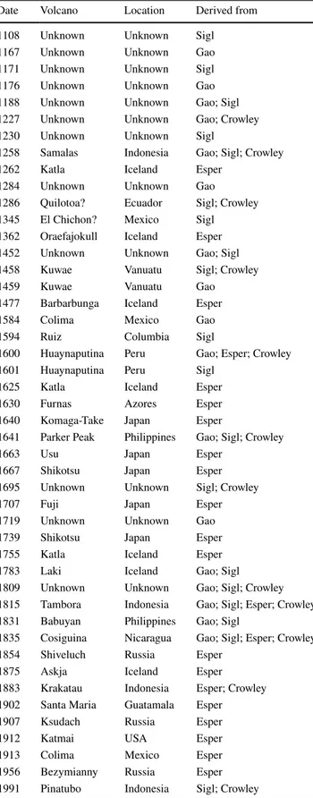
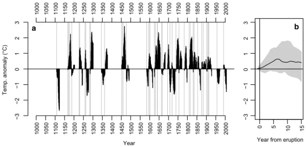
To verify whether the isotope ratios show the same sen-sitivity to volcanic eruptions as the ring width, we first compared the responses from their independent LF recon-structions (i.e., based on a single proxy) to each of the 46 strong volcanic eruptions listed in Table 1 (Fig. 5). These eruptions were derived from Gao et al. (2008), Crowley and Unterman (2013), Esper et al. (2013) or Sigl et al. (2013, 2015). In the figure, the y-axis shows the subtraction between the post-eruption anomalies reconstructed from isotope ratios (average anomalies from δ18O and δ13C) and from ring width. Positive (negative) values indicate that post-eruption anomalies are more negative in the recon-struction from ring width (isotope ratios). We can thus see that ring width indexes often reconstruct more negative temperature anomalies after volcanic events (Fig. 5b) than isotopic proxies, confirming the different proxy sensitivity to volcanic forcing. However, the variability of responses after different eruptions is large. Indeed different volcano locations, atmospheric states during the eruptions, event intensities and days of the year may cause specific impacts over the Quebec-Labrador peninsula, which are more or less registered by the proxies.
Subsequently, we focused on the three periods of the last millennium where the volcanic impact should have been the strongest and for which Gennaretti et al. (2014) found significant regime shifts toward lower growth values in the ring width chronologies. These periods are the thirteenth century with the series of eruptions centered around the 1258 Samalas event and that supposedly triggered the onset of the LIA; the second half of the fifteenth century with the cooling episode following the 1458–1459 Kuwae eruption; and the first half of the nineteenth century, probably the coldest period of the last millennium in the Quebec taiga, with a series of eruptions centered around the 1815 Tamb-ora event. This analysis (Fig. 6) reveals that δ13C of spruce trees growing on lakeshores is almost insensitive to vol-canic impacts. It is also clear that ring width shows much more important volcanic impacts than δ18O, reconstructing the strongest coolings after single events and the strong-est cumulative impacts from multiple events. Interstrong-estingly, during the thirteenth century at the onset of the LIA, all three proxies agree in reconstructing an overall cooling trend despite the amplitude of the trend and short-term tem-perature variations depending on the proxies. In this case, the impact of individual eruptions appears not correlated to their intensity. Indeed, following the 1258 Samalas erup-tion, which was likely the strongest of the last millennium
Table 1 List of 46 eruption years derived from Gao et al. (2008; global total stratospheric sulfate aerosol injection > 15Tg), Crowley
and Unterman (2013; satellite aerosol optical depth > 0.1), Esper et al.
(2013; eruptions classified as large events) or Sigl et al. (2013, 2015;
eruptions classified as large events)
Date Volcano Location Derived from
1108 Unknown Unknown Sigl
1167 Unknown Unknown Gao
1171 Unknown Unknown Sigl
1176 Unknown Unknown Gao
1188 Unknown Unknown Gao; Sigl
1227 Unknown Unknown Gao; Crowley
1230 Unknown Unknown Sigl
1258 Samalas Indonesia Gao; Sigl; Crowley
1262 Katla Iceland Esper
1284 Unknown Unknown Gao
1286 Quilotoa? Ecuador Sigl; Crowley
1345 El Chichon? Mexico Sigl
1362 Oraefajokull Iceland Esper
1452 Unknown Unknown Gao; Sigl
1458 Kuwae Vanuatu Sigl; Crowley
1459 Kuwae Vanuatu Gao
1477 Barbarbunga Iceland Esper
1584 Colima Mexico Gao
1594 Ruiz Columbia Sigl
1600 Huaynaputina Peru Gao; Esper; Crowley
1601 Huaynaputina Peru Sigl
1625 Katla Iceland Esper
1630 Furnas Azores Esper
1640 Komaga-Take Japan Esper
1641 Parker Peak Philippines Gao; Sigl; Crowley
1663 Usu Japan Esper
1667 Shikotsu Japan Esper
1695 Unknown Unknown Sigl; Crowley
1707 Fuji Japan Esper
1719 Unknown Unknown Gao
1739 Shikotsu Japan Esper
1755 Katla Iceland Esper
1783 Laki Iceland Gao; Sigl
1809 Unknown Unknown Gao; Sigl; Crowley
1815 Tambora Indonesia Gao; Sigl; Esper; Crowley
1831 Babuyan Philippines Gao; Sigl
1835 Cosiguina Nicaragua Gao; Sigl; Esper; Crowley
1854 Shiveluch Russia Esper
1875 Askja Iceland Esper
1883 Krakatau Indonesia Esper; Crowley
1902 Santa Maria Guatamala Esper
1907 Ksudach Russia Esper
1912 Katmai USA Esper
1913 Colima Mexico Esper
1956 Bezymianny Russia Esper
(Lavigne et al. 2013), the proxies react as after other strong eruptions of the same period. During the second half of the fifteenth century, δ18O and ring width strongly disagree in the volcanic responses. While δ18O shows only moder-ate coolings (approximmoder-ately −0.5 °C) lasting for no more than 3 years after the two strong eruptions of 1452 and 1458–1459, ring width displays an important cumulative impact of these two events, culminating in anomalies of approximately −3.5 °C (note that this discussion on cooling intensities and durations is based on smoothed data because only low frequencies are available for isotope ratios due to the data processing method). A good proxy agreement is instead observed during the first half of the nineteenth cen-tury where the decadal trends in δ18O and ring width are very similar despite ring width again showing larger tem-perature variations. The LF 3P-STREC reconstruction with the ensemble of the proxies always has an intermediate behavior between the δ18O and the ring width reconstruc-tions with a preference towards δ18O which is likely the better estimate of past temperatures.
As this comparison of the proxy differential sensi-tivity to volcanic eruptions showed that ring width LFs responded more strongly than isotopic ones, it is possible that the ring width component of 3P-STREC amplifies the volcanic forcing after strong eruptions (see Büntgen et al.
2015). This may be the case especially in cold periods, such as the Little Ice Age, and/or if the time between suc-cessive eruptions is short (Sigl et al. 2013). Indeed, in cold periods with recurrent volcano-induced temperature reduc-tions, tree growth is likely to suffer from the depletion of carbohydrate reserves and from the fact that the tissues and
canopy can be frost-damaged. Conversely, it is also possi-ble that the isotopic proxies are less sensitive to the meteor-ological perturbations related to volcanic events. Latewood maximum density data, which nevertheless could also have their limitations (see Stine and Huybers 2014; Tingley et al. 2014), may be useful to discriminate between these hypotheses.
4 Conclusion
In this paper, we presented the first annually resolved and millennium-long multiproxy temperature reconstruction for northeastern North America based on tree-ring width and stable isotope ratios (δ13C and δ18O). The climate informa-tion embedded in the three proxies was exploited using a Bayesian framework that allows for a rigorous uncertainty assessment. The results showed that the final reconstruc-tion 3P-STREC was a clear improvement over previous attempts based only on ring width or δ18O values. Using the Bayesian methodology, we can also provide reliable confidence intervals that are much sharper than simply merging the three independent reconstructions from sin-gle proxies. At the moment, 3P-STREC represents the best estimate of the past summer temperature of our region (the mean of July–August temperature), but in the future, the results could be further improved by (1) adding additional proxies (e.g., ring maximum density) to reduce the remain-ing sources of LF errors and improve the HF calibration, (2) considering more complex mechanistic modeling of the proxy-climate relationships, (3) providing a more robust
−3 −2 −1 01 2 3 1000 1050 1100 1150 1200 1250 1300 1350 1400 1450 1500 1550 1600 1650 1700 1750 1800 1850 1900 1950 2000 1000 1050 1100 1150 1200 1250 1300 1350 1400 1450 1500 1550 1600 1650 1700 1750 1800 1850 1900 1950 2000 Year Temp. anomaly (°C) a 0 5 10 15 −3 −2 −1 0123
Year from eruption
b
Fig. 5 Comparison of responses from low frequency reconstructions
based on ring width and isotopic proxies to individual strong volcanic
eruptions of the last millennium (listed in Table 1). Plot a shows if
the anomalies of each 15 post-eruption years (anomalies relative to the year before the eruption) are more negative in the
reconstruc-tion from ring width (positive values) or from stable isotope ratios
(negative values; average anomalies from δ18O and δ13C). Eruption
years are vertical lines. Plot b shows a Superimposed Epoch Analy-sis (median and 60% confidence intervals) based on the data and the eruption years of plot a
intra- and inter-site-explicit uncertainty analysis, or (4) tak-ing into account the year to year memory of each compo-nent in the model as a fractional Gaussian process (Lovejoy et al. 2015) in order to properly integrate the information from different sources (Li et al. 2010) and investigate the impact of higher long-term persistence in ring width data compared to instrumental data (Zhang et al. 2015). How-ever, concerning this last point, we want to stress out that 3P-STREC is already shown to be well calibrated in the LF domain.
We also examined different proxy sensitivities to cli-mate forcing, focusing the analysis on the impact of vol-canic eruptions. The reconstruction from ring width had a larger and longer response to single or consecutive erup-tions, while those from isotope ratios showed an interme-diate (δ18O) or nearly absent (δ13C) volcanic impact. It is
difficult to know the real influence of past volcanic events on temperature at the regional scale because many uncer-tainties exist due to (1) the limited knowledge on the mechanisms behind the proxy responses, (2) the absence of major volcanic events during the period when the proxies are compared with instrumental data, (3) the low agreement in the volcanic datasets concerning timing and respective forcing of eruptions (Crowley and Unterman
2013; Esper et al. 2013; Gao et al. 2008; Sigl et al. 2013,
2015), and (4) the complexity of comparing the results of proxy-based reconstructions with simulations of past climate with plausible initial conditions, sulfate aerosols and ocean feedback (circulation, sea ice, relaxation time of subsurface temperature and sea level) during volcanic coolings (Stenchikov et al. 2009). In our reconstruc-tion, the uncertainties came from the specific reduced
1180 1200 1220 1240 1260 1280 1300 −5 −4 −3 −2 −1 0 1 Year Te mp. anomalies (°C) 0.00 0.04 0.08 0.12 pdf
(a) Volcanic impact during the 13th century
1450 1460 1470 1480 1490 −5 −4 −3 −2 −1 0 1 Year Te mp. anomalies (°C) 0.00 0.04 0.08 0.12 pdf
(b) Volcanic impact during the second half of the 15th century
1810 1820 1830 1840 1850 −5 −4 −3 −2 −1 0 1 Year Te mp. anomalies (°C ) 0.00 0.04 0.08 0.12 pdf
(c) Volcanic impact during the first half of the 19th century
Fig. 6 Proxy response during periods of strong volcanic impact: the
thirteenth century (a), the second half of the fifteenth century (b) and the first half of the nineteenth century (c). Temperature anomalies with respect to the first considered year are shown on the left of each panel (medians and 90% confidence intervals), and anomaly posterior densities of the year with lowest anomalies are shown on the right
(the selected year is highlighted by a vertical gray bar on the left plots). Black colors for the proxy ensemble low frequency reconstruc-tion 3P-STREC, red for the reconstrucreconstruc-tion using ring width only, blue
for δ18O and green for δ13C. Vertical dotted lines and arrows indicate
or amplified responses to volcanic eruptions of the three temperature-sensitive proxies. We should bear in mind that each proxy has its advantages and drawbacks. Only a multi-proxy approach can allow us to take advantage of the proxy convergence and reduce individual sources of error caused by specific mechanistic responses of the proxies.
Acknowledgements This project has received funding from the
European Union’s Horizon 2020 research and innovation programme under the Marie Sklodowska-Curie grant agreement No 656896. The
δ13C series has been produced through the support of the
Environ-mental Geoscience program of the Geological Survey of Canada.
Open Access This article is distributed under the terms of the
Creative Commons Attribution 4.0 International License (http://
creativecommons.org/licenses/by/4.0/), which permits unrestricted use, distribution, and reproduction in any medium, provided you give appropriate credit to the original author(s) and the source, provide a link to the Creative Commons license, and indicate if changes were made.
References
Arseneault D, Dy B, Gennaretti F, Autin J, Bégin Y (2013) Devel-oping millennial tree ring chronologies in the fire-prone North
American boreal forest. J Quat Sci 28:283–292. doi:10.1002/
jqs.2612
Autin J, Gennaretti F, Arseneault D, Bégin Y (2015) Biases in RCS tree ring chronologies due to sampling heights of trees.
Dendro-chronologia 36:13–22. doi:10.1016/j.dendro.2015.08.002
Boucher E, Guiot J, Chapron E (2011) A millennial multi-proxy reconstruction of summer PDSI for Southern South America.
Clim Past 7:957–974. doi:10.5194/cp-7-957-2011
Büntgen U, Trouet V, Frank D, Leuschner HH, Friedrichs D, Luter-bacher J, Esper J (2010) Tree-ring indicators of German summer drought over the last millennium. Quat Sci Rev 29:1005–1016. doi:10.1016/j.quascirev.2010.01.003
Büntgen U et al (2011) 2500 years of European climate variability
and human susceptibility. Science 331:578–582. doi:10.1126/
science.1197175
Büntgen U et al (2015) Tree-ring amplification of the early nine-teenth-century summer cooling in Central Europe. J Clim
28:5272–5288. doi:10.1175/jcli-d-14-00673.1
Crowley TJ, Unterman MB (2013) Technical details concerning development of a 1200 year proxy index for global volcanism.
Earth Syst Sci Data 5:187–197. doi:10.5194/essd-5-187-2013
D’arrigo RD, Jacoby GC (1993) Secular trends in high northern latitude temperature reconstructions based on tree rings. Clim
Change 25:163–177. doi:10.1007/BF01661204
D’Arrigo R, Wilson R, Anchukaitis KJ (2013) Volcanic cooling signal in tree ring temperature records for the past millennium. J
Geo-phys Res D Atmos 118:9000–9010. doi:10.1002/jgrd.50692
Emile-Geay J, Tingley M (2016) Inferring climate variability from nonlinear proxies: application to palaeo-ENSO studies. Clim
Past 12:31–50. doi:10.5194/cp-12-31-2016
Esper J et al (2012) Orbital forcing of tree-ring data. Nat Clim Change
2:862–866. doi:10.1038/nclimate1589
Esper J et al. (2013) European summer temperature response to annu-ally dated volcanic eruptions over the past nine centuries. Bull
Volcanol 75:1–14. doi:10.1007/s00445-013-0736-z
Esper J, Schneider L, Smerdon JE, Schöne BR, Büntgen U (2015) Signals and memory in tree-ring width and density data.
Dendro-chronologia 35:62–70. doi:10.1016/j.dendro.2015.07.001
Esper J et al. (2016) Ranking of tree-ring based temperature recon-structions of the past millennium. Quat Sci Rev 145:134–151. doi:10.1016/j.quascirev.2016.05.009
Farquhar GD, O’Leary MH, Berry JA (1982) On the relationship between carbon isotope discrimination and the intercellular car-bon dioxide concentration in leaves. Aust J Plant Physiol 9:121–
137. doi:10.1071/PP9820121
Fischer EM, Luterbacher J, Zorita E, Tett SFB, Casty C, Wanner H (2007) European climate response to tropical volcanic eruptions over the last half millennium. Geophys Res Lett 34:L05707. doi:
10.1029/2006gl027992
Francey RJ, Farquhar GD (1982) An explanation of 13 C/12 C
varia-tions in tree rings. Nature 297:28–31. doi:10.1038/297028a0
Gagen M et al (2011) Cloud response to summer temperatures in Fennoscandia over the last thousand years. Geophys Res Lett
38:L05701. doi:10.1029/2010gl046216
Gagen M, McCarroll D, Jalkanen R, Loader NJ, Robertson I, Young GHF (2012) A rapid method for the production of robust mil-lennial length stable isotope tree ring series for climate
recon-struction. Global Planet Change 82–83:96–103. doi:10.1016/j.
gloplacha.2011.11.006
Gao C, Robock A, Ammann C (2008) Volcanic forcing of climate over the past 1500 years: an improved ice core-based index for
climate models. J Geophys Res Atmos 113:D23111. doi:10.10
29/2008jd010239
Gennaretti F, Arseneault D, Nicault A, Perreault L, Bégin Y (2014) Volcano-induced regime shifts in millennial tree-ring chronol-ogies from northeastern North America. Proc Natl Acad Sci
USA 111:10077–10082. doi:10.1073/pnas.1324220111
Harris I, Jones PD, Osborn TJ, Lister DH (2014) Updated high-resolution grids of monthly climatic observations—the CRU
TS3.10 Dataset. Int J Climatol 34:623–642. doi:10.1002/
joc.3711
Kaufman DS et al (2009) Recent warming reverses long-term arctic
cooling. Science 325:1236–1239. doi:10.1126/science.1173983
Kruschke JK (2014) Doing Bayesian data analysis: a tutorial with R, JAGS, and Stan, 2nd edn. Elsevier Science, Amsterdam. doi:10.1016/b978-0-12-405888-0.09999-2
Lavigne F et al (2013) Source of the great A.D. 1257 mystery eruption unveiled, Samalas volcano, Rinjani Volcanic Complex,
Indone-sia. Proc Natl Acad Sci USA 110:16742–16747. doi:10.1073/
pnas.1307520110
Li B, Nychka DW, Ammann CM (2010) The value of multiproxy reconstruction of past climate. J Am Stat Assoc 105:883–895. doi:10.1198/jasa.2010.ap09379
Lovejoy S, Del Rio Amador L, Hébert R (2015) The ScaLIng Mac-roweather Model (SLIMM): using scaling to forecast global-scale macroweather from months to decades. Earth Syst Dyn
6:637–658. doi:10.5194/esd-6-637-2015
Luterbacher J et al. (2016) European summer tempera-tures since Roman times. Environ Res Lett 11:024001. doi:10.1088/1748-9326/11/2/024001
Mann ME et al (2009) Global signatures and dynamical origins of the little ice age and medieval climate anomaly. Science 326:1256–
1260. doi:10.1126/science.1177303
Matskovsky VV, Helama S (2014) Testing long-term summer tem-perature reconstruction based on maximum density chronologies obtained by reanalysis of tree-ring data sets from northernmost
Sweden and Finland. Clim Past 10:1473–1487. doi:10.5194/
cp-10-1473-2014
McCarroll D, Loader NJ (2004) Stable isotopes in tree rings. Quat Sci
McCarroll D et al. (2009) Correction of tree ring stable carbon iso-tope chronologies for changes in the carbon dioxide content of the atmosphere. Geochim Cosmochim Acta 73:1539–1547. doi:10.1016/j.gca.2008.11.041
McCarroll D et al (2013) A 1200-year multiproxy record of tree growth and summer temperature at the north-ern pine forest limit of Europe. Holocene 23:471–484. doi:10.1177/0959683612467483
Melvin TM, Grudd H, Briffa KR (2013) Potential bias in ‘updating’ tree-ring chronologies using regional curve standardisation: re-processing 1500 years of Torneträsk density and ring-width data.
Holocene 23:364–373. doi:10.1177/0959683612460791
Miller GH et al (2012) Abrupt onset of the Little Ice Age triggered by volcanism and sustained by sea-ice/ocean feedbacks. Geophys
Res Lett 39:L02708. doi:10.1029/2011gl050168
Miller GH, Lehman SJ, Refsnider KA, Southon JR, Zhong Y (2013) Unprecedented recent summer warmth in Arctic Canada.
Geo-phys Res Lett 40:5745–5751. doi:10.1002/2013gl057188
Naulier M, Savard MM, Bégin C, Marion J, Arseneault D, Bégin Y (2014) Carbon and oxygen isotopes of lakeshore black spruce trees in northeastern Canada as proxies for climatic
reconstruction. Chem Geol 374–375:37–43. doi:10.1016/j.
chemgeo.2014.02.031
Naulier M et al. (2015) A millennial summer temperature reconstruc-tion for northeastern Canada using oxygen isotopes in subfossil
trees. Clim Past 11:1153–1164. doi:10.5194/cp-11-1153-2015
Pages 2k Consortium (2013) Continental-scale temperature vari-ability during the past two millennia. Nat Geosci 6:339–346. doi:10.1038/ngeo1797
Robock A (2005) Cooling following large volcanic eruptions cor-rected for the effect of diffuse radiation on tree rings. Geophys
Res Lett 32:1–4. doi:10.1029/2004gl022116
Schleussner CF, Feulner G (2013) A volcanically triggered regime shift in the subpolar North Atlantic Ocean as a possible
ori-gin of the Little Ice Age. Clim Past 9:1321–1330. doi:10.5194/
cp-9-1321-2013
Schneider L, Smerdon JE, Büntgen U, Wilson RJS, Myglan VS, Kirdyanov AV, Esper J (2015) Revising midlatitude summer temperatures back to A.D. 600 based on a wood density network.
Geophys Res Lett 42:GL063956. doi:10.1002/2015gl063956
Sidorova OV et al. (2012) A multi-proxy approach for revealing recent climatic changes in the Russian Altai. Clim Dyn 38:175–
188. doi:10.1007/s00382-010-0989-6
Sidorova OV et al (2013) The application of tree-rings and sta-ble isotopes for reconstructions of climate conditions in the
Russian Altai. Clim Change 120:153–167. doi:10.1007/
s10584-013-0805-5
Sigl M et al (2013) A new bipolar ice core record of volcanism from WAIS divide and NEEM and implications for climate forcing of
the last 2000 years. J Geophys Res Atmos 118:1151–1169. doi:1
0.1029/2012jd018603
Sigl M et al (2015) Timing and climate forcing of volcanic
erup-tions for the past 2,500 years. Nature 523:543–549. doi:10.1038/
nature14565
Stenchikov G, Delworth TL, Ramaswamy V, Stouffer RJ, Wittenberg A, Zeng F (2009) Volcanic signals in oceans. J Geophys Res
Atmos 114:D16104. doi:10.1029/2008jd011673
Stine AR, Huybers P (2014) Arctic tree rings as recorders of
varia-tions in light availability. Nat Commun 5:1–8. doi:10.1038/
ncomms4836
Stoffel M et al. (2015) Estimates of volcanic-induced cooling in the Northern Hemisphere over the past 1,500 years. Nat Geosci
8:784–788. doi:10.1038/ngeo2526
Tierney JE, Tingley MP (2014) A Bayesian, spatially-varying cali-bration model for the TEX86 proxy. Geochim Cosmochim Acta
127:83–106. doi:10.1016/j.gca.2013.11.026
Tingley MP, Huybers P (2010) A Bayesian algorithm for reconstruct-ing climate anomalies in space and time. Part I: development and applications to paleoclimate reconstruction problems. J Clim
23:2759–2781. doi:10.1175/2009JCLI3015.1
Tingley MP, Stine AR, Huybers P (2014) Temperature reconstruc-tions from tree-ring densities overestimate volcanic cooling.
Geophys Res Lett 41:7838–7845. doi:10.1002/2014gl061268
Tolwinski-Ward SE, Anchukaitis KJ, Evans MN (2013) Bayes-ian parameter estimation and interpretation for an intermediate
model of tree-ring width. Clim Past 9:1481–1493. doi:10.5194/
cp-9-1481-2013
Tolwinski-Ward SE, Tingley MP, Evans MN, Hughes MK, Nychka DW (2015) Probabilistic reconstructions of local temperature and soil moisture from tree-ring data with potentially
time-varying climatic response. Clim Dyn 44:791–806. doi:10.1007/
s00382-014-2139-z
van Albada SJ, Robinson PA (2007) Transformation of arbitrary distributions to the normal distribution with application to EEG test–retest reliability. J Neurosci Meth 161:205–211. doi:10.1016/j.jneumeth.2006.11.004
Viau AE, Ladd M, Gajewski K (2012) The climate of North America during the past 2000 years reconstructed from
pol-len data. Global Planet Change 84–85:75–83. doi:10.1016/j.
gloplacha.2011.09.010
Wilson R et al. (2016) Last millennium northern hemisphere summer temperatures from tree rings: part I: the long term context. Quat
Sci Rev 134:1–18. doi:10.1016/j.quascirev.2015.12.005
Young GHF, McCarroll D, Loader NJ, Kirchhefer AJ (2010) A 500-year record of summer near-ground solar radiation from tree-ring stable carbon isotopes. Holocene 20:315–324. doi:10.1177/0959683609351902
Zanchettin D et al. (2012) Bi-decadal variability excited in the cou-pled ocean-atmosphere system by strong tropical volcanic
erup-tions. Clim Dyn 39:419–444. doi:10.1007/s00382-011-1167-1
Zhang H et al. (2015) Modified climate with long term mem-ory in tree ring proxies. Environ Res Lett 10:084020. doi:10.1088/1748-9326/10/8/084020
Zhong Y, Miller GH, Otto-Bliesner BL, Holland MM, Bailey DA, Schneider DP, Geirsdottir A (2011) Centennial-scale climate change from decadally-paced explosive volcanism: a coupled sea
ice-ocean mechanism. Clim Dyn 37:2373–2387. doi:10.1007/