HAL Id: hal-00302099
https://hal.archives-ouvertes.fr/hal-00302099
Submitted on 5 Sep 2006HAL is a multi-disciplinary open access
archive for the deposit and dissemination of sci-entific research documents, whether they are pub-lished or not. The documents may come from teaching and research institutions in France or abroad, or from public or private research centers.
L’archive ouverte pluridisciplinaire HAL, est destinée au dépôt et à la diffusion de documents scientifiques de niveau recherche, publiés ou non, émanant des établissements d’enseignement et de recherche français ou étrangers, des laboratoires publics ou privés.
The January 2006 low ozone event over the UK
M. Keil, D. R. Jackson, M. C. Hort
To cite this version:
M. Keil, D. R. Jackson, M. C. Hort. The January 2006 low ozone event over the UK. Atmospheric Chemistry and Physics Discussions, European Geosciences Union, 2006, 6 (5), pp.8457-8483. �hal-00302099�
ACPD
6, 8457–8483, 2006
Low ozone over the UK M. Keil et al. Title Page Abstract Introduction Conclusions References Tables Figures J I J I Back Close
Full Screen / Esc
Printer-friendly Version Interactive Discussion
EGU
Atmos. Chem. Phys. Discuss., 6, 8457–8483, 2006 www.atmos-chem-phys-discuss.net/6/8457/2006/ © Author(s) 2006. This work is licensed
under a Creative Commons License.
Atmospheric Chemistry and Physics Discussions
The January 2006 low ozone event over
the UK
M. Keil, D. R. Jackson, and M. C. Hort
Met Office, FitzRoy Road, Exeter, EX1 3PB, UK
Received: 7 July 2006 – Accepted: 3 August – Published: 5 September 2006 Correspondence to: M. Keil ([email protected])
ACPD
6, 8457–8483, 2006
Low ozone over the UK M. Keil et al. Title Page Abstract Introduction Conclusions References Tables Figures J I J I Back Close
Full Screen / Esc
Printer-friendly Version Interactive Discussion
EGU
Abstract
A record low total ozone column of 177 DU was observed at Reading, UK, on 19 Jan-uary 2006. Low ozone values were also recorded at other stations in the British Isles and North West Europe on, and around, this date. Hemispheric maps of total ozone from the World Meteorological Organisation (WMO) Ozone Mapping Centre also show
5
the evolution of this ozone minimum from 15–20 January 2006 over North West Eu-rope.
Ozonesonde measurements made at Lerwick, UK, show that ozone mixing ratios in the mid-stratosphere on 18 January are around 1–2 ppmv lower than both climatology and observations made one and two weeks prior to this date. In addition, ozone mixing
10
ratios in the UTLS region were also noticeably reduced on 18 January. Analysis of the ozonesonde observations indicate that the mid-stratosphere ozone accounts for around a third of the reduction in total ozone column measurements while the UTLS ozone values account for two thirds of the depletion. It is evident from the ozonesonde data that ozone loss is occuring at two distinct vertical regions.
15
Met Office analyses indicate that stratospheric polar vortex temperatures were cold enough for Polar Stratospheric Cloud (PSC) formation during 14 days in January prior to the low ozone event on 19 January. The presence of PSCs is confirmed by observa-tions from the Scanning Imaging Absorption spectroMeter for Atmospheric Cartogra-pHY (SCIAMACHY). As a consequence of a stratospheric sudden warming that was in
20
progress during January 2006, the polar vortex was shifted southwards over northwest Europe. This includes a period from 16 to 19 January where PSCs were present in the vortex over the UK. Throughout most of January suitable conditions were present for ozone destruction by heterogenous chemistry within the polar vortex. Evidence from Lerwick and Sodankyl ¨a ozonesonde profiles, and maps of Ertel’s potential vorticity
cal-25
culated from Met Office analyses, strongly suggests that the air inside the stratospheric vortex was poor in ozone for at least one week prior to 18 January. It is also possible that local chemical destruction of stratospheric ozone further contributed to the record
ACPD
6, 8457–8483, 2006
Low ozone over the UK M. Keil et al. Title Page Abstract Introduction Conclusions References Tables Figures J I J I Back Close
Full Screen / Esc
Printer-friendly Version Interactive Discussion
EGU
low ozone observed at Reading.
A closer examination of the WMO total ozone maps shows that the daily minima are often of synoptic, rather than planetary, scale. This therefore suggests a tropospheric, rather than stratospheric, mechanism for the ozone minima. Moderate total ozone depletion is commonly observed in the northern hemisphere middle and high latitude
5
winter. This depletion is related to the lifting of the tropopause associated with the presence of an upper troposphere/lower stratosphere anticyclone. We show a strong link between the ozone minima in the WMO maps and 100 hPa geopotential height from Met Office analyses, and therefore it appears that this may also be a plausible mechanism for the record low ozone column that is observed.
10
Back trajectories calculated by the Met Office NAME III model show that air parcels in the mid-stratosphere do arrive over the British Isles on 19 January via the polar vortex. The NAME III model results also show that air parcels near the tropopause arrive from low latitudes and are transported anticyclonically. Therefore this strongly suggests that the record low ozone values are due to a combination of a raised tropopause and the
15
presence of low ozone stratospheric air aloft.
1 Introduction
It is well-known that column total ozone levels undergo fluctuations associated with the passage of tropospheric weather systems. Cases where depletion occurs are often referred to as “ozone mini-holes” and have been documented by a number of authors
20
e.g.Newman et al.(1988),McKenna et al.(1989),Peters et al.(1995),James(1998).
The ozone depletion results from the presence of an anticyclone in the upper tropo-sphere/lower stratosphere (UTLS). The associated raising of the tropopause means that a greater proportion of the column is occupied by ozone-poor tropospheric air. In addition, the divergence of ozone-rich air out of the column in the lower stratosphere
25
leads to a further reduction in total ozone.
ACPD
6, 8457–8483, 2006
Low ozone over the UK M. Keil et al. Title Page Abstract Introduction Conclusions References Tables Figures J I J I Back Close
Full Screen / Esc
Printer-friendly Version Interactive Discussion
EGU 1998), and a smaller number of very intense mini holes are often observed in
com-bination with a sudden stratospheric warming or other distortion of the stratospheric polar vortex. Case studies of such events include Petzoldt et al.(1994) and Petzoldt
(1999). In these events the very cold temperatures within the vortex lead to chemical destruction of stratospheric ozone, and the horizontal advection of this ozone-poor air
5
over a region where the ozone column is already reduced due to the presence of a UTLS anticyclone leads to an even larger reduction in the total ozone column.
Allen et al. (2002) reported a total ozone column of 165 DU on 30 November 1999
over Europe observed by the Total Ozone Mapping Spectrometer (TOMS). This is a record for this instrument and this location. In January 2006 a total ozone measurement
10
of 177 DU was observed over Reading, UK, which is a record low for the ground-based instruments used at this and at other UK sites. Allen and Nakamura used a tracer transport model to reconstruct the ozone field in November 1999 and thus to determine the mechanism that caused the very low ozone column over Europe. Here, we instead use back trajectories calculated from the Met Office NAME III dispersion
15
model to investigate the events of January 2006. Hitherto, the NAME III model has primarily been used to investigate tropospheric pollution in a wide range of applications ranging from the dispersion of nuclear contamination and volcanic ash to the prediction of air quality levels based on thousands of UK and European anthropogenic and natural emissions. The results presented here show that the NAME III model can also be very
20
effective at diagnosing events in the stratosphere.
The outline of the paper is as follows. In Sect. 2 the low ozone event is described via UK ground-based total ozone measurements, hemispheric maps of World Mete-orological Organisation (WMO) Ozone Mapping Centre total ozone, and ozonesonde profiles from Lerwick, UK. The meteorological situation in the stratosphere and near
25
the tropopause is described in Sect. 3 and is used to interpret the patterns shown in the ozone measurements. Then in Sect. 4 back trajectory calculations from the NAME III model are used to determine the origin of the air parcels that arrived at the low ozone column ozone observed at Reading. Conclusions appear in Sect. 5.
ACPD
6, 8457–8483, 2006
Low ozone over the UK M. Keil et al. Title Page Abstract Introduction Conclusions References Tables Figures J I J I Back Close
Full Screen / Esc
Printer-friendly Version Interactive Discussion
EGU
2 Observations of the low ozone event
We start by presenting observations made over the UK by Dobson spectrophotometers at Lerwick (60.13◦N, 1.18◦W), Camborne (50.13◦N, 5.18◦W) and Bracknell (51.38◦N, 0.78◦W) and by a Brewer spectrophotometer at Reading (51.46◦N, 0.97◦W). The Ler-wick observations used are from January 1979–present, the Reading observations
5
from January 2003–present, and the Camborne and Bracknell observations are a com-bined dataset that spans November 1989 to December 2003.
The retrieval accuracy of the Dobson instrument should be around ±1% in direct sun conditions. However, since the observations were made in January, when the sun is low, the accuracy is likely to have been ±4% (Komhyr,1980). The retrieval accuracy
10
of a well-maintained Brewer spectrophotometer is ±1% and its precision is better than ±1% (Gao et al.,2001).
At Reading, like in much of the northern hemisphere, minimum total ozone is ob-served between November and February. Figure 1 shows 2005/06 observations for these months and the daily maximum and minimum values from the 2002/03 to 2004/05
15
winters. The minimum value recorded is 177 DU on 19 January 2006. This is more than 100 DU less than the minimum for 19 January for the previous observed winters and is also clearly less than the daily minimum for any other day in the November to February period (apart from the observation on 18 January 2006).
The dataset at Reading is too short to adequately represent interannual
variabil-20
ity and therefore to gain an indication of this, we look at the daily maxima and minima from the 14 year long record from Camborne/Bracknell. These locations are sufficiently close to Reading for us to assume they approximately represent the 1989–2003 clima-tology for Reading. Figure 1 shows that the daily minimum for Camborne/Bracknell on 19 January is less than that observed at Reading, but it is still over 50 DU greater than
25
the observation at Reading on 19 January 2006.
Figure 1 also shows total ozone observations at Lerwick, which is approximately 10◦ latitude north of Reading. It can be seen that the minimum total ozone for 2005/06 is
ACPD
6, 8457–8483, 2006
Low ozone over the UK M. Keil et al. Title Page Abstract Introduction Conclusions References Tables Figures J I J I Back Close
Full Screen / Esc
Printer-friendly Version Interactive Discussion
EGU
observed on 18 January, one day before the minimum at Reading. Although this is a new low for the climatology envelope for this date, this minimum is less remarkable as it is fairly similar to other daily minima from the 1979–2005 record.
In order to gain a better idea of the spatial pattern of this total ozone event, we now look at daily maps of hemispheric total ozone. The maps are obtained from the WMO
5
Ozone Mapping Centre (http://lap.physics.auth.gr/ozonemaps). The maps are created by assimilating total ozone data from the Scanning Imaging Absorption spectroMeter for Atmospheric CartograpHY (SCIAMACHY) using a transport model (Eskes et al.,
2003). The SCIAMACHY total ozone columns are retrieved using the TOSOMI algo-rithm, which is described byEskes et al. (2005). Validation shows a bias of around
10
−1.5% compared to Global Ozone Mapping Experiment (GOME) and ground-based observations.
Figure 2 shows daily WMO ozone maps from 15–20 January 2006. Broadly speak-ing, in the extratropics the low ozone is in a region whose southernmost extent is in middle latitudes between the central North Atlantic and Russia and which narrows with
15
increasing latitude and extends to north of Scandinavia. Met Office analyses of middle stratosphere geopotential height and Ertel’s potential vorticity for these dates shows that the stratospheric vortex has been displaced from the pole and is present in ap-proximately the same location as the total ozone minimum described above.
The total ozone maps also show that, within the large low ozone region, the ozone
20
distribution varies on the synoptic scale. For example, on 19 January there are two regions of high ozone in the north Atlantic and over eastern Europe and a region of lower ozone in between. This pattern is indicative of a change in column ozone related to the passage of tropospheric weather systems.
To get a better idea of what is happening to the vertical distribution of ozone, we now
25
move away from total column observations to look at ozone profiles measured by a Met Office ozonesonde at Lerwick. The sonde is of the Electrochemical Concentration Cell (ECC) type. The total error for ECC sondes is estimated to be within −7% to+17% in the upper troposphere, ±5% in the lower stratosphere up to 10 hPa and −14% to
ACPD
6, 8457–8483, 2006
Low ozone over the UK M. Keil et al. Title Page Abstract Introduction Conclusions References Tables Figures J I J I Back Close
Full Screen / Esc
Printer-friendly Version Interactive Discussion
EGU
+6% at 4 hPa (Komhyr et al.,1995). Errors are higher in the presence of steep ozone gradients and where ozone amounts are low.
During winter, the sonde usually makes one ascent per week. Figure 3 shows that on 18 January 2006 ozone mixing ratios between 50 and 10 hPa are around 3–3.5 ppmv. This is up to 2 ppmv less than corresponding values from observations made on 4
5
and 11 January 2006 and also around 1 ppmv lower than the January climatology of Lerwick radiosonde ascents. This means that ozone-poor stratospheric air is being transported over Lerwick on 18 January and/or ozone destruction is taking place in the cold stratosphere above Lerwick on that date. Also shown in Fig. 3 are ozonesonde profiles from Sodankyl ¨a, Finland (67.35◦N, 26.63◦E) on similar dates. Between around
10
50 and 10 hPa the ozone profiles on 5 and 18 January at Sodankyl ¨a are broadly similar to those on 4 and 18 January, respectively, at Lerwick. The relationship between these observations and the location of the polar vortex will be discussed further in Sect. 3.
At lower altitudes, at around 200–80 hPa, the ozone values at Lerwick are up to 1 ppmv lower than climatology for both 4 and 18 January. This indicates that additional
15
processes are occurring in the upper troposphere lower stratosphere region that af-fect the total column. Conversion from mixing ratio to total column ozone reveals that approximately a third of the depletion in the total ozone column (w.r.t the January cli-matology) originates from the stratospheric 50–10 hPa region, while two thirds comes from the UTLS 200–80 hPa region. This analysis confirms that important ozone
deplet-20
ing processes occur in two distinct regions and they are discussed further in the next section.
3 Meteorological situation
In this section we use daily Met Office stratospheric analyses (Swinbank et al.,2004) to describe the meteorological situation in January 2006. Unlike the cold, undisturbed
25
Northern Hemisphere winter of 2004/5, the stratosphere has been dynamically dis-turbed in 2005/6. In mid January there was a minor stratospheric warming, which
ACPD
6, 8457–8483, 2006
Low ozone over the UK M. Keil et al. Title Page Abstract Introduction Conclusions References Tables Figures J I J I Back Close
Full Screen / Esc
Printer-friendly Version Interactive Discussion
EGU
became a major warming on 21 January and persisted until early February. A major stratospheric warming occurs when the temperature gradient at 10 hPa (around 30 km) between 60◦N and the pole is reversed to become warmer at the pole. In addition the polar night jet reverses from westerly to easterly at 60◦N and 10 hPa. The January 2006 warming led to a significant displacement of the polar night vortex away from the
5
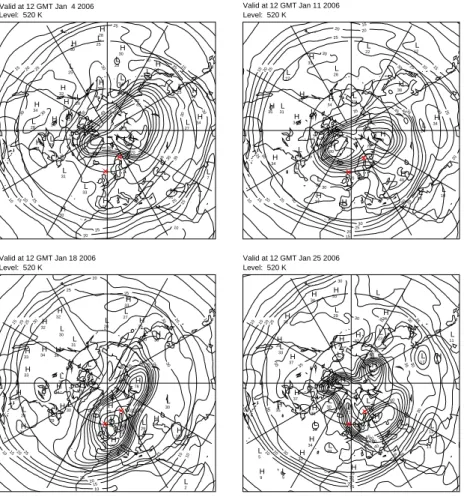
pole. The intensity and duration of this major warming are greater than average. The typical meteorological situation for a cold, undisturbed, January (such as in 2005) is a near-zonally symmetric polar vortex, centred near the pole and with associ-ated cold temperatures. The analyses from January 2006 show a very different picture. Figure 4 shows Ertel’s potential vorticity on the 520 K isentropic surface (approximately
10
50 hPa) for selected days in January 2006. During the course of the month the vor-tex becomes increasingly distorted and moves southwards and eastwards across the North Atlantic and Northern Europe.
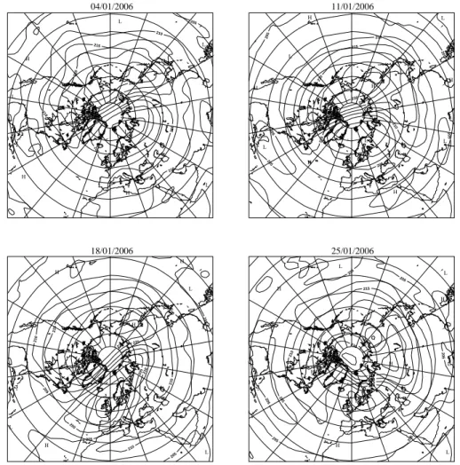
The southward movement of the vortex also implies southward movement of the cold air within it. This is reflected in Fig. 5 which is similar to Fig. 4, except that temperatures
15
at 46 hPa are shown. By 18 January minimum temperatures of less than 195 K are located over the British Isles. From then until 25 January this cold air is transported eastward across the British Isles and into central Europe.
Met Office analyses show that for 14 out of the first 19 days in January critical thresh-olds for Polar Stratospheric Cloud (PSC) formation are exceeded within the polar
vor-20
tex. PSCs at similar locations are also seen in SCIAMACHY observations (von Savigny
et al.,2005) on these days (data available from:http://www-iup.physik.uni-bremen.de/ ∼sciaproc/PSC/PSC 2006 S00.html). The presence of PSCs coupled with the fact that
the vortex has moved during this period from a region of reduced sunlight to an area of greater sunlight allow conditions for heterogeneous chemical destruction of ozone to
25
be met.
The low temperatures and the presence of PSCs during January indicate that the air within the polar vortex is likely to be ozone poor prior to 18 January. The low ozone air observed at Lerwick on 18 January is simply a result of Lerwick being inside the polar
ACPD
6, 8457–8483, 2006
Low ozone over the UK M. Keil et al. Title Page Abstract Introduction Conclusions References Tables Figures J I J I Back Close
Full Screen / Esc
Printer-friendly Version Interactive Discussion
EGU
vortex on that date, rather than as a consequence of local heteregeneous chemical destruction of ozone. Figure 4 does indeed strongly suggest that both Lerwick and Sodankyl ¨a are inside the polar vortex on 18 January and outside it on 4 January. The observed stratosphere ozone at these sites is considerably lower on the former date than on the latter. Furthermore, on 11 January Lerwick is also outside the vortex
5
and the lower stratospheric ozone values are similar to those on 4 January, whilst Sodankyl ¨a is on the edge of the vortex and ozone values are clearly lower than on 5 January (though not quite as low as on 18 January). This strongly suggests that for at least a week before 18 January, stratospheric ozone inside the vortex was depleted. Maps of Ertel’s potential vorticity also show that Reading is within the stratospheric
10
polar vortex on 19 January (not shown) and so it appears that the presence of ozone poor stratosphere vortex air would contribute to the record low ozone column observed at Reading on that date.
Of course, without detailed chemical modelling studies it is hard to quantify how much of the ozone depletion at Lerwick on 18 January is pre-existing and how much is
15
due to local heteregeneous chemical destruction associated with the presence of the PSCs implied by Fig. 5. This is outside the scope of this study.
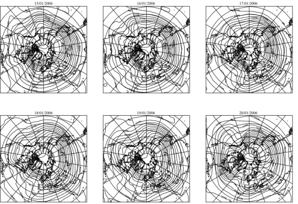
As indicated in Sects. 1 and 2, another possible mechanism for a reduction in total ozone column is the raising of the tropopause associated with a UTLS anticyclone. Figure 6 shows geopotential height at 100 hPa from Met Office analyses for 15–20
20
January 2006. Focusing on the middle latitudes between the central North Atlantic and Russia, we see that there is a clear link between anticyclones (cyclones), which can be seen as ridges (troughs) in Fig. 7, and depletions (enhancements) in the SCIAMACHY total ozone columns (Fig. 2). In addition, these features can also be associated with the surface pressure fields (not shown). In particular, the strong ridging pattern in
25
the 100 hPa geopotential height fields can be related to large surface high pressure systems.
The origin of the ozone minimum over the British Isles on 19 January is seen on 16 January. On that date there are ozone minima over the central North Atlantic and
ACPD
6, 8457–8483, 2006
Low ozone over the UK M. Keil et al. Title Page Abstract Introduction Conclusions References Tables Figures J I J I Back Close
Full Screen / Esc
Printer-friendly Version Interactive Discussion
EGU
Scandinavia which are associated with anticyclones in these regions. The Atlantic anticyclone moves eastward over the next few days, reaching the British Isles on 19 January, and the associated eastward movement of the ozone minimum can be seen in Fig. 2. By 20 January a low pressure system appears to the north of the British Isles, with an associated rise in ozone column (seen as a trough in Fig. 6). In subsequent
5
days there is a continued fall/rise in total ozone over the British Isles associated with the passage of anticyclones/cyclones, but the very low ozone column seen on 18 and 19 January is not observed again.
Similar synoptic situations to those described are seen in the Met Office 100 hPa geopotential height fields in early January 2006. However, it is interesting that the
10
SCIAMACHY fields do not show such a deep minimum in total ozone on these dates. This is confirmed by the ground-based observations in Fig. 1. This suggests that the very low ozone columns on 18 and 19 January are due to a combination of the pres-ence of a UTLS anticyclone and of ozone depletion aloft.
4 NAME III model simulations
15
In order to investigate the origin of stratospheric air back trajectories were run using the Met Office’s dispersion model, NAME III, which is a Lagrangian particle trajec-tory model (Ryall and Maryon, 1998; Jones et al., 2005). Emissions from pollutant sources are represented by particles released into a model atmosphere driven by the meteorological fields from the Met Office’s numerical weather prediction model, the
20
Unified Model (Davies et al.,2005). Each particle carries mass of one or more pollu-tant species. These are advected by the local mean wind, with various random walk techniques used to represent turbulent diffusion processes. Parameterizations also represent processes such as the entrainment between the boundary layer and the free troposphere, and for the mixing by deep convection. The particles also evolve through
25
processes such as wet and dry deposition, sedimentation and chemical destruction and creation. The model is routinely used in a wide range of applications: examples
ACPD
6, 8457–8483, 2006
Low ozone over the UK M. Keil et al. Title Page Abstract Introduction Conclusions References Tables Figures J I J I Back Close
Full Screen / Esc
Printer-friendly Version Interactive Discussion
EGU
include the prediction of air quality levels based on thousands of UK and European anthropogenic and natural emissions, the transport and deposition of debris following the Chernobyl accident (Smith and Clark,1989) and the airborne spread of foot and mouth disease during the epidemic in the UK in 2001 (Gloster et al.,2001).
In addition, a key advantage of utilizing a Lagrangian approach for dispersion
model-5
ing is the ability to run the model backwards in time and thereby enable the identification of source-receptor relationships (Manning et al.,2003). This capability makes it possi-ble to identify the origin (both time and location) of all particles reaching a location at any given time. It is in this configuration that the model has been used here.
Simulations with the NAME III model were run to investigate the origins of the air
10
making up the low ozone columns seen in the WMO maps in Fig. 2. A receptor was defined and then simulations were run backwards in time for 7 days from the receptor date. NAME III was driven by the analysis fields from the Met Office operational global weather prediction model, with the top of the domain being restricted to 30 km. A number of low ozone events are shown in Fig. 2. We choose to investigate the low
15
ozone region seen near Reading on 19 January 2006. Accordingly, a receptor was defined at 51.46◦N 0.97◦W on that date.
In order to assist in understanding the results a series of simulations were carried out using an receptor measuring 100 km2 in the horizontal and extending from 10 km to 30 km in altitude. The receptor was then repositioned at 5 different horizontal
lo-20
cations (North, South, East, West and Central) covering the extent of the observed low ozone feature. This series of simulations was designed to enable the determina-tion of the sensitivity of our specificadetermina-tion and also to reduce the amount of possible information for any given prediction. Results for all the different horizontal locations are very consistent. This indicates that, over an area of 10◦ in latitude and longitude
25
centred at 51.46◦N 0.97◦W (the low ozone area), the simulations are spatially robust. Accordingly, all plots included here are for the central location.
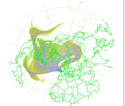
Figure 7 shows the integrated concentration over the first five days of the back trajec-tory run over the whole vertical domain. Much of the air mass arriving at the receptor
ACPD
6, 8457–8483, 2006
Low ozone over the UK M. Keil et al. Title Page Abstract Introduction Conclusions References Tables Figures J I J I Back Close
Full Screen / Esc
Printer-friendly Version Interactive Discussion
EGU
originates in a ring between Iceland and North West Russia. Comparisons with Met Office stratospheric Ertel’s potential vorticity maps for January (Fig. 4) suggest that this flow is very similar to the flow of the stratospheric polar vortex. In order to better de-termine the origins of the air, further plots are shown which only feature air arriving at the receptor from certain atmospheric layers. Figure 8 is similar to Fig. 7, except that it
5
only shows air arriving at the receptor that is in the 15–30 km layer. This confirms that this ring of air is stratospheric in origin.
Figure 7 also shows air originating from other locations, such as the Pacific and the northern subtropical Atlantic. Figure 8 shows that little or none of this air originates from the 15–30 km layer, so in order to determine the origin of this air, further vertical
10
slices at 5–10 km and 10–15 km were examined, and these are shown in Figs. 9 and 10, respectively. These plots give a clear picture of both southerly and vertical transport.
Figure 9 indicates that most of the air in the 10–15 km layer that subsequently arrives at the receptor location is not polar vortex in origin. The flow is very similar in pattern to the geopotential height fields at 100 hPa in Fig. 6 and can be seen to follow an
anti-15
cyclonic path to the receptor region. Figure 10 shows that there is also a volume of air originating in the northern subtropical Atlantic from an altitude between 5 km and 10 km that took 3–5 days to arrive at the receptor location. This air also follows an anti-cyclonic path as it approaches the receptor region.
We can see from Figs. 7–10 that air arriving at the receptor region has two main
20
sources. Air in the 15–30 km region is primarily stratospheric vortex in origin, with very little transport from elsewhere. In the previous section we showed that this air is likely to be ozone poor prior to arriving over the British Isles on 18 and 19 January. In the 5–10 km and 10–15 km layers, the air arriving at the receptor is likely to have undergone horizontal and vertical transport related to the passage of UTLS cyclones
25
and anticyclones shown in Fig. 6. Close to the receptor, the flow regime is anticyclonic which is consistent with a raised tropopause and, accordingly, a decrease in the total ozone column. These results were in agreement with other NAME runs based on receptor regions for the low ozone area on 17 and 18 January. These additional runs
ACPD
6, 8457–8483, 2006
Low ozone over the UK M. Keil et al. Title Page Abstract Introduction Conclusions References Tables Figures J I J I Back Close
Full Screen / Esc
Printer-friendly Version Interactive Discussion
EGU
produced consistent results with air transported to the receptor region from similar areas.
5 Conclusions
A record low total column ozone value of 177 DU was observed at Reading, UK on 19 January 2006. Ozonesonde observations from Lerwick show a large depletion in
mid-5
stratospheric ozone between 50 and 10 hPa around this date. In addition, there was a noticeable decrease in the ozone around the UTLS, 200–80 hPa, region. Analysis of the ozonesonde data indicates that one third of the depletion in the total ozone column originates from the middle stratosphere, while the reduction in UTLS ozone values contributes towards the rest of the depletion. This indicates that important ozone
10
depleting processes were at work in two different regions.
Met Office analyses shows that at this time the stratospheric polar vortex was dis-placed over the British Isles. Evidence from Lerwick and Sodankyl ¨a ozonesondes, and Met Office fields of Ertel’s potential vorticity, suggests that the British Isles was within the stratospheric vortex at this time and that the air within the vortex was already ozone
15
poor. This low ozone air would contribute to the record low ozone column observed at Reading. The temperatures within the vortex were low enough to cause PSC formation and thus local ozone destruction via heterogeneous chemistry, and it is a possibility that this could further add to the ozone depletion. However, without using a chemical model it is impossible to quantify how much ozone depletion could come from this source.
20
WMO total ozone maps show a large region of low ozone approximately colocated with the displaced polar vortex. However, they also show a smaller, synoptic, scale pattern to the ozone column depletion in middle latitudes. This points to another cause for the low ozone over the British Isles, namely the impact of UTLS anticyclones in reducing the total ozone column. These events are well documented, see e.g.Newman 25
et al. (1988);McKenna et al.(1989);Peters et al.(1995);James(1998), and frequently observed. They occur because associated with the presence of the anticyclone is a
ACPD
6, 8457–8483, 2006
Low ozone over the UK M. Keil et al. Title Page Abstract Introduction Conclusions References Tables Figures J I J I Back Close
Full Screen / Esc
Printer-friendly Version Interactive Discussion
EGU
raising of the tropopause, meaning that a greater proportion of the column is occupied by ozone-poor tropospheric air. In addition, the divergence of ozone-rich air out of the column in the lower stratosphere leads to a further reduction in total ozone. We have shown that there is a strong link between the patterns of total ozone minima seen in the WMO maps and the location of anticyclones in 100 hPa geopotential height fields
5
from Met Office analyses. Therefore, it appears that this mechanism also contributes to the record low ozone columns observed.
In order to determine the origin of the ozone poor air we use simulations from the NAME III model. The results show that middle stratosphere air has been transported in the polar vortex from higher latitudes from the region of lowest temperatures, and this
10
adds further weight to the hypothesis that this air will have undergone ozone destruction due to heterogeneous chemistry prior to reaching the region of observed low ozone in mid latitudes. The model results also show that air is transported to the receptor point from near-tropopause levels (5–15 km) in an anticyclonic path. This pattern is consisted with what is shown in Met Office analyses of geopotential height at 100 hPa
15
and WMO total ozone maps. It clearly confirms that the synoptic scale reductions in ozone seen in these maps is associated with the raising of the tropopause that occurs in the presence of these UTLS anticyclones.
It is important to note the possible health impacts of such decreased ozone events.
Austin et al.(1999) reported record low ozone in late April/early May 1997 over
south-20
ern England. The erythemally-weighted ultraviolet levels recorded at this time were similar to those normally recorded in June or July, and the impacts on human health of exposure to this abnormally high amount of radiation are clear. Similarly,Stick et al.
(2006) reported unusually large UV values over northern Germany in May 2005 as a result of an ozone mini-hole. The event in January 2006 that we have reported may
25
have some impact on the biosphere, but is unlikely to have many consequences for hu-man health since erythemally-weighted ultraviolet levels do not usually start to become significant at middle or high latitudes until around a month after the spring equinox.
ACPD
6, 8457–8483, 2006
Low ozone over the UK M. Keil et al. Title Page Abstract Introduction Conclusions References Tables Figures J I J I Back Close
Full Screen / Esc
Printer-friendly Version Interactive Discussion
EGU
assimilated ozone fields to the WMO ozone mapping centre. D. Moore provided Met Office ozonesonde data and his knowledge of the observations was extremely helpful. Sodankyl ¨a ozonesonde data were obtained from the NILU database. Netcen provided the UK surface observations from Reading and Lerwick on behalf of DEFRA. Comments from a number of Met Office colleagues resulted in considerable improvements to this study.
5
References
Allen, D. R. and Nakamura, N.: Dynamical reconstruction of the record low column ozone over Europe on 30 November 1999, Geophys. Res. Lett., 29, 1362, doi:10.1029/2002GL014935,
2002. 8460
Austin, J., Driscoll, C. M. H., Farmer, S. F. G., and Molyneux, M. J.: Late spring ultraviolet levels
10
over the United Kingdom and the link to ozone, Ann. Geophys., 17, 1199–1209, 1999. 8470
Davies, T., Cullen, M. J. P., Malcolm, A. J., Mawson, M. H., Staniforth, A., White, A. A., and Wood, N.: A new dynamical core for the Met Office’s global and regional modelling of the atmosphere, Quart. J. Roy. Meteorol. Soc., 131, 1759–1782, 2005. 8466
Eskes, H. J., van Velthoven, P. F. J., Valks, P. J. M., and Kelder, H. E.: Assimilation of GOME
15
total ozone satellite observations in a three-dimensional tracer transport model, Quart. J. Roy. Meteorol. Soc., 129, 1663–1681, 2003 8462
Eskes, H. J., van der A, R. J., Brinksma, E. J., Veefkind, J. P., de Haan, J. F., and Valks, P. J. M.: Retrieval and validation of ozone columns derived from measurements of SCIAMACHY on Envisat, Atmos. Chem. Phys. Discuss., 5, 4429–4475, 2005. 8462
20
Gao, W., Slusser, J., Gibson, J., Scott, G., Bigelow, D., Kerr, J., and McArthur, B.: Direct-Sun column ozone retrieval by the ultraviolet multifilter rotating shadow-band radiometer and comparison with those from Brewer and Dobson spectrophotometers, Appl. Optics, 40, 3149–3155, 2001. 8461
Gloster J., Champion H. J., Mansley L. M., Romero P., Brough, T., and Ramirez A.: The 2001
25
epidemic of foot-and-mouth disease in the United Kingdom: epidemiological and meteoro-logical case studies, The Veterinary Record, 156, 793–803, 2001. 8467
James, P. M.: A climatology of ozone mini-holes over the northern hemisphere, Int. J. Climatol-ogy, 18, 1287–1303, 1998. 8459,8469
Jones, A., Thomson, D., Hort, M., and Devenish, B.: The U. K. Met Office’s next generation
ACPD
6, 8457–8483, 2006
Low ozone over the UK M. Keil et al. Title Page Abstract Introduction Conclusions References Tables Figures J I J I Back Close
Full Screen / Esc
Printer-friendly Version Interactive Discussion
EGU
mospheric dispersion model NAME III, Air pollution modeling and its application XVII, edited by: Borrego, C. and Norman, A., in press, Springer, 2006. 8466
Komhyr, W. D.: Ozone Observations with a Dobson Spectrophotometer, WMO Global Ozone Research and Monitoring Project Report No. 6, NOAA Environmental Research Laborato-ries, 1980. 8461
5
Komhyr, W. D., Barnes, R. A., Brothers, G. B., Lathrop, J. A., and Opperman, D. P.: Elec-trochemical Concentration Cell ozonesonde performance evaluation during STOIC 1989, J. Geophys. Res., 100, 9231–9244, 1995. 8463
Manning, A. J., Ryall, D. B., Derwent, R. G., Simmonds, P. G., and O’Doherty, S.: Estimating Eu-ropean emissions of ozone-depleting and greenhouse gases using observations and a
mod-10
elling back-attribution technique, J. Geophys. Res., 108, 4405, doi:10.029/2002JD002312,
2003. 8467
McKenna, D. S., Jones, R. L., Austin, J., Browell, E. V., McCormick, M. P., Krueger, A. J., and Tuck, A. F.: Diagnostic studies of the Antarctic vortex during the 1987 Airborne Antarctic Ozone Experiment – ozone miniholes, J. Geophys. Res., 94, 11 641–11 668, 1989. 8459,
15
8469
Newman, P. A., Lait, L. A., and Schoeberl, M. R.: The morphology and meteorology of southern-hemisphere spring total ozone mini-holes, Geophys. Res. Lett., 15, 923–926, 1988.
8459,8469
Peters, D., Egger, J., and Entzian, G.: Dynamical aspects of ozone mini-hole formation,
Mete-20
orol. Atmos. Phys., 55, 205–214, 1995. 8459,8469
Petzoldt, K., Naujokat, B., and Neugeboren, K.: Coorelation between stratospheric tempera-ture, total ozone, and tropospheric weather systems, Geophys. Res. Lett., 21, 1203–1206,
1994. 8460
Petzoldt, K.: The role of dynamics in total ozone deviations from their long-term mean over the
25
Northern Hemisphere, Ann. Geophys., 17, 231–241, 1999. 8460
Ryall, D. B. and Maryon, R. H.: Validation of the UK Met. Office’s NAME model against the ETEX dataset (1998), Atmospheric Environment, 32, 4265–4276, 1998. 8466
Stick, C., Kr ¨uger, K., Schade, N. H., Sandmann, H., and Macke, A.: Episode of unusually high solar ultraviolet radiation over central Europe due to dynamical reduced total ozone in May
30
2005, Atmos. Chem. Phys., 6, 1771–1776, 2006. 8470
Smith, F. B. and Clark, M. J.: The transport and deposition of airborne debris from the Cher-nobyl nuclear power plant accident with special emphasis on the consequences to the United
ACPD
6, 8457–8483, 2006
Low ozone over the UK M. Keil et al. Title Page Abstract Introduction Conclusions References Tables Figures J I J I Back Close
Full Screen / Esc
Printer-friendly Version Interactive Discussion
EGU
Kingdom, Meteorological Office Scientific Paper No. 42, HMSO (available from Met Office, FitzRoy Road, Exeter EX1 3PB, UK), 1989. 8467
Swinbank, R., Keil, M., Jackson, D. R., and Scaife, A. A.: Stratospheric Data Assimilation at the Met Office – progress and plans. ECMWF workshop on Modelling and Assimilation for the Stratosphere and Tropopause, 23–26 June 2003, 2004 8463
5
von Savigny, C., Ulasi, E. P., Eichmann, K. U., Bovensmann, H., and Burrows, J. P.: Detection and mapping of polar stratospheric clouds using limb scattering observations, Atmos. Chem. Phys., 5, 3071–3079, 2005. 8464
ACPD
6, 8457–8483, 2006
Low ozone over the UK M. Keil et al. Title Page Abstract Introduction Conclusions References Tables Figures J I J I Back Close
Full Screen / Esc
Printer-friendly Version Interactive Discussion
EGU
Fig. 1. Total ozone observations between 1 November and 29 February. Top panel:
ob-servations at Reading between 1 November 2005 and 28 February 2006 (asterisks), daily maximum and minimum total ozone at Reading from January 2003–February 2005 data (solid lines), daily maximum and minimum total ozone at Camborne/Bracknell from 1989–2003 data (dashed lines). Bottom panel: observations at Lerwick between 1 November 2005 and 28 February 2006 (asterisks), daily maximum and minimum total ozone at Lerwick from January 1979–February 2005 data (solid lines).
ACPD
6, 8457–8483, 2006
Low ozone over the UK M. Keil et al. Title Page Abstract Introduction Conclusions References Tables Figures J I J I Back Close
Full Screen / Esc
Printer-friendly Version Interactive Discussion
EGU
ACPD
6, 8457–8483, 2006
Low ozone over the UK M. Keil et al. Title Page Abstract Introduction Conclusions References Tables Figures J I J I Back Close
Full Screen / Esc
Printer-friendly Version Interactive Discussion
EGU
Fig. 3. Ozone profiles measured by ozonesondes at Lerwick on the left hand plot and
So-dankyl ¨a, Finland, on the right hand plot. The red line corresponds to 4 and 5 January 2006 for Lerwick and Sodankyl ¨a, respectively, the green line 11 January 2006, the black line 18 January 2006. The January climatology of Lerwick radiosonde ascents is shown in blue on both plots (dashed represents ±1σ). Units: ppmv.
ACPD
6, 8457–8483, 2006
Low ozone over the UK M. Keil et al. Title Page Abstract Introduction Conclusions References Tables Figures J I J I Back Close
Full Screen / Esc
Printer-friendly Version Interactive Discussion EGU Valid at 12 GMT Jan 18 2006 Valid at 12 GMT Jan 11 2006 Valid at 12 GMT Jan 25 2006 Valid at 12 GMT Jan 4 2006 Level: 520 K Level: 520 K Level: 520 K Level: 520 K H H L H 28 33 22 33 H L H L 32 12 34 25 L H L H 27 33 19 30 H L L H 32 28 29 30 L L H L 28 27 34 H H H 25 H 35 38 32 L H H 34 L 30 33 35 L L H 25 L 30 27 37 H H L 25 L 36 34 23 L H L 24 H 31 35 11 H L H 36 H 34 31 35 H L H 32 L 34 30 37 H H L 25 H 33 34 33 H H H 31 L 35 34 37 L L L 26 H 29 24 29 H H L 34 H 33 79 17 L H H 33 32 80 31 L H L H 25 78 30 80 H L H H 34 28 34 74 H H L L 34 34 30 30 L L H H 28 29 49 37 L H L L 27 33 28 30 L L L L 29 30 10 50 H H L H 80 34 14 35 H L H H 38 30 37 71 L H H H 31 79 35 36 L L H 7 28 78 L L L 33 29 29 L L H 15 6 64 72 L H L 36 34 13 H L H 31 29 34 H H L 41 31 13 H H L 30 78 29 H 20 L 32 5 H H 20 79 33 L H 2 35 H 25 9 L 5 25 20 25 30 25 30 15 30 2025 30 25 15 20 20 30 15 25 30 2515 1520 2530 30 10 20 15 15 20 25 30 30 3025 35 30 35 40 45 40 35 30 25 4555 55 45 35 30 60 35 65 40 30 45 30 35 4050 60 30 30 35 35 3530 70 70 60 25 30 50 35 20 60 70 7060 50 40 70 65 35 403530 60 15 30 30 30 35 10 1520 25 30 30 20 10 15 20 10 25 25 15 15 2025 25 15 10 15 40 20 45 25 50 30 55 20 25 60 65 10 10 15 20 25 1020 30 3020 15 202530
Fig. 4. PV on the 520 K theta surface (approx. 50 hPa) derived from Met Office analyses on 4
January 2006 (top left), 11 January 2006 (top right), 18 January 2006 (bottom left), 25 January 2006 (bottom right). Contour interval 5 PV units. Crosses mark the locations of Lerwick and Sodankyl ¨a.
ACPD
6, 8457–8483, 2006
Low ozone over the UK M. Keil et al. Title Page Abstract Introduction Conclusions References Tables Figures J I J I Back Close
Full Screen / Esc
Printer-friendly Version Interactive Discussion EGU H H H H L L L L L 200 205 205 210 210 210 210 215 215 220 220 225 H H H H H H L L L L L 205 205 205 205 205 205 210 210 04/01/2006 18/01/2006 25/01/2006 11/01/2006 210 215 215 220 220 225 230 H H H H H L L L L L 200 205 205 205 205 205 210 210 210 210 215 215 220 225 H H H H H L L L L L L 205 205 205 205 205 205 205 210 210 210 215 215 220 220 225 225 230
Fig. 5. Temperature at 46 hPa from Met Office analysis on 4 January 2006 (top left), 11 January
2006 (top right), 18 January 2006 (bottom left), 25 January 2006 (bottom right). Contour interval 5 K.
ACPD
6, 8457–8483, 2006
Low ozone over the UK M. Keil et al. Title Page Abstract Introduction Conclusions References Tables Figures J I J I Back Close
Full Screen / Esc
Printer-friendly Version Interactive Discussion EGU 15400. 15500. 15600. 15600. 15700. 15700. 15800. 15800. 15900. 15900. 16000. 16000. 16100. 16100. 16100. 16200. 16200. 16200. 16300. 16300. 16300. 16400. 16400. 16400. 16500. 16500. 16500. 15200. 15300. 15400. 15/01/2006 18/01/2006 19/01/2006 15500. 15600. 15700. 15700. 15800. 15800. 15900. 15900. 16000. 16000. 16100. 16100. 16200. 16200. 16200. 16300. 16300. 16300. 16400. 16400. 16400. 16500. 16500. 16500. 15200. 15300. 15400. 15500. 15600. 15700. 15700. 15800. 15800. 15900. 15900. 16000. 16000. 16100. 16100. 16200. 16200. 16200. 16300. 16300. 16300. 16400. 16400. 16400. 16500. 16500. 16500. 15300. 15400. 15500. 15600. 15700. 15700. 15800. 15800. 15900. 15900. 16000. 16000. 16100. 16100. 16100. 16200. 16200. 16300. 16300. 16400. 16400. 16400. 16500. 16500. 16500. 15400. 15500. 15600. 15700. 15700. 15800. 15800. 15900. 15900. 16000. 16000. 16100. 16100. 16200. 16200. 16300. 16300. 16300. 16400. 16400. 16400. 16500. 16500. 16600. 15400. 15500. 15500. 15600. 15700. 15800. 15800. 15900. 15900. 16000. 16000. 16000. 16100. 16100. 16200. 16200. 16200. 16300. 16300. 16300. 16400. 16400. 16400. 16500. 16500. 16500. 16500. 16/01/2006 17/01/2006 20/01/2006
Fig. 6. Geopotential height at 100 hPa from Met Office analyses on 15 January 2006 (top left),
16 January 2006 (top centre), 17 January 2006 (top right), 18 January 2006 (bottom left), 19 January 2006 (bottom centre) and 20 January 2006 (bottom right). Contour interval: 10 dam.
ACPD
6, 8457–8483, 2006
Low ozone over the UK M. Keil et al. Title Page Abstract Introduction Conclusions References Tables Figures J I J I Back Close
Full Screen / Esc
Printer-friendly Version Interactive Discussion
EGU 1.00e−11 1.00e−10 1.00e−09 1.00e−08 1.00e−07 1.00e−06
Maximum value = 1.24e−07
Fig. 7. NAME III derived five day air history map for parcels originating in the 0–30 km vertical
region from a receptor of 100 km2 horizontal area with a 10–30 km vertical extent centred on 51.46◦N, 0.97◦W (black cross). The contours represent the time integrated air concentration from each grid box (dx,dy,dz) that contributes to the receptor on 19 January 2006 between 11:00 and 13:00 UTC given a release rate of 1 g/s.
ACPD
6, 8457–8483, 2006
Low ozone over the UK M. Keil et al. Title Page Abstract Introduction Conclusions References Tables Figures J I J I Back Close
Full Screen / Esc
Printer-friendly Version Interactive Discussion
EGU 1.00e−11 1.00e−10 1.00e−09 1.00e−08 1.00e−07 1.00e−06
Maximum value = 2.04e−07
Fig. 8. As previous figure, except results are shown for air originating from the 15–30 km
ACPD
6, 8457–8483, 2006
Low ozone over the UK M. Keil et al. Title Page Abstract Introduction Conclusions References Tables Figures J I J I Back Close
Full Screen / Esc
Printer-friendly Version Interactive Discussion
EGU 1.00e−11 1.00e−10 1.00e−09 1.00e−08 1.00e−07 1.00e−06
Maximum value = 1.32e−07
ACPD
6, 8457–8483, 2006
Low ozone over the UK M. Keil et al. Title Page Abstract Introduction Conclusions References Tables Figures J I J I Back Close
Full Screen / Esc
Printer-friendly Version Interactive Discussion EGU 10 30 50 70 80 60 40 20 0 20
1.00e−11 1.00e−10 1.00e−09 1.00e−08 1.00e−07 1.00e−06 Maximum value = 2.90e−08