Computational time-resolved imaging

(1)

Computational Time-resolved Imaging

by

Ghulam A. Kirmani

S.M., Media Technology

Massachusetts Institute of Technology, 2010

Integrated M.Tech in Mathematics and Computing

ARCHNE

MASSACHUSETTS INSTITUTE OF TECHNOLOLGY

MAR 19

2015

LIBRARIES

Indian Institute of Technology Delhi, 2008

Submitted to the

Department of Electrical Engineering and Computer Science

in partial fulfillment of the requirements for the degree of

Doctor of Philosophy in Electrical Engineering and Computer Science

at the

MASSACHUSETTS INSTITUTE OF TECHNOLOGY

February 2015

Massachusetts Institute of Technology 2015. All rights reserved.

Signature redacted

A u th or ...

...

Department of Electrical EngineerFig and Computer Science

Certified by

0 nh

'In- I Mu

Signature redacted

mber 15, 2014

Certified by

Jeffrey H. Shapiro

Julius A. Stratton Professor of Electrical Engineering

Massachusetts Institute of Technology

j

/,,

Th'iis

Supervisor

Signature redacted

... ...

r

Vivek

K

Goyal

Assistant Professor of Electrical and Computer Engineering

Boston University

A ccepted by ...

-

. t, . , .

. Thesis Supervisor

Signature redacted...

I'

sl'i4 A. Kolodziejski

Chair, Department Committee on Graduate Students

(2)

(3)

Computational Time-resolved Imaging

by

Ghulam A. Kirmani

Submitted to the Department of Electrical Engineering and Computer Science on December 15, 2014, in partial fulfillment of the

requirements for the degree of

Doctor of Philosophy in Electrical Engineering and Computer Science

Abstract

Classical photography uses steady-state illumination and light sensing with focusing optics to capture scene reflectivity as images; temporal variations of the light field are not exploited. This thesis explores the use of time-varying optical illumination and time-resolved sensing along with signal modeling and computational reconstruction. Its purpose is to create new imaging modalities, and to demonstrate high-quality imaging in cases in which traditional techniques fail to even form degraded imagery. The principal contributions in this thesis are the derivation of physically-accurate signal models for the scene's response to time-varying illumination and the photodetection statistics of the sensor, and the combining of these models with computationally tractable signal recovery algorithms leading to image formation.

In active optical imaging setups, we use computational time-resolved imaging to exper-imentally demonstrate: non line-of-sight imaging or looking around corners, in which only diffusely scattered light was used to image a hidden plane which was completely occluded from both the light source and the sensor; single-pixel 3D imaging or compressive depth ac-quisition, in which accurate depth maps were obtained using a single, non-spatially resolving bucket detector in combination with a spatial light modulator; and high-photon efficiency imaging including first-photon imaging, in which high-quality 3D and reflectivity images were formed using only the first detected photon at each sensor pixel despite the presence

of high levels of background light.

Thesis Supervisor: Jeffrey H. Shapiro

Title: Julius A. Stratton Professor of Electrical Engineering Massachusetts Institute of Technology

Thesis Supervisor: Vivek K Goyal

Title: Assistant Professor of Electrical and Computer Engineering Boston University

(4)

(5)

Acknowledgments

The work in this thesis has been the culmination of the support and inspiration I derived from many people throughout my academic career. But my experience in the doctoral program itself has been very enriching in many dimensions which I credit to the stimulating environment at MIT, and in particular at the Research Laboratory of Electronics. I would like to express my gratitude to each person who made my time here so much more meaningful and interesting.

To my advisor Vivek Goyal, for accepting me to the doctoral program in EECS and welcoming me to his group even before I was officially a graduate student in the department. I am very grateful for his patience and strong support to new ideas, and for truly manifesting that the sky is the limit for any willing and eager graduate student and for fighting hurdles to support his students' interests even when it meant he had to go out of his way. As the leader of the Signal Transformation and Information Representation group, he created

an environment complete with resources, collaborators, opportunities and encouragement there was no excuse for a STIR member to not try hard problems. I would like to thank him for this unique work environment he created and maintained.

To my advisor in the second half of my doctoral program, Jeff Shapiro, who has been a great mentor with very valuable critic at every step. Through his principled and rigorous

approach to optical problems, I have become more a rigorous researcher myself.

In my graduate school career I had the unfortunate or fortunate experience of academic-style differences that escalated to unnecessary conflict. I am grateful to Jeff for helping me navigate these challenges and for teaching me the invaluable lesson of doing the right thing even when the situation is seemingly not in your favor. His judgment and wisdom will be an important part of my learning.

To my thesis reader Pablo Parrilo for his rigorous research and teaching style, and for teaching me that the devil is in the little details when it comes to doing good research. He was my inspiration to come to MIT for graduate school.

To my collaborators in the Optical and Quantum Communications Group, Dr. Franco Wong and Dheera Venkatraman for their insightful contributions to experiments in this

(6)

thesis. I am grateful to them for their willingness to share lab space and equipment which strongly supplemented all the theoretical work and provided concrete experimental results.

To the leaders in signal processing, optimization and information theory with whom I have had several opportunities to interact and learn from Professors Sanjoy Mitter, John Tsitsitklis, Devavrat Shah, George Verghese, Yury Polyanskiy, Moe Win, Greg Wornell.

To the STIR family of students Lav Varshney, Dan Weller, John Sun, Joong Bum Rhim for being great team members, for sharing their grad school experiences with me and brainstorming ideas with me when I was new to the group. To STIR fellow-student Dongeek Shin with whom I collaborated intensely for two years, who diligently found creative solutions to our research problems, and for many stimulating discussions on theoretical bounds to various problems we investigated together. I would also like to thank my collaborator Hye Soo Yang for all her help and expertise. I especially thank Andrea Colago for embarking on many undefined problems and experiments with me when we first began work on 3D optical imaging in the STIR group, and for being a wise mentor on several key occasions. Several other friends at MIT have made my time really memorable and fun. I would like to thank Parikshit Shah, Vaibhav Rathi, Noah Stein, Raghavendra Hosur, Anirudh Sarkar, and Aditya Bhakta for the good times.

I dedicate this thesis to the memory of my late father who would have been very happy and proud today. I would also like to thank my mother for her infinite patience and support, my grandparents who raised me with great love and care and provided the best opportunities at every step, and my younger brother and sister who have been such wonderful supporters and lifelong friends.

This work in this thesis was supported by the U.S. NSF under grant numbers 1161413, 0643836 and 1422034, a Qualcomim Innovation Fellowship, a Microsoft Research Ph.D. Fel-lowship, and a Texas Instrument research grant.

(7)

Chapter 1 Introduction

The goal of imaging is to produce a representation in one-to-one spatial correspondence with an object or scene. For centuries, the primary technical meaning of image has been a visual representation formed through the interaction of light with mirrors and lenses, and recorded through a photochemical process. In digital photography, the photochemical process has been replaced by an electronic sensor array, but the use of optical elements is unchanged. Conventional imaging for capturing scene reflectivity, or photography, uses natural illumination and light sensing with focusing optics; variations of the light field with time are not exploited.

A brief history of time in optical imaging: Figure 1-1 shows a progression of key events which depict the increasing exploitation of temporal information contained in optical signals to form 3D and reflectivity images of a scene. The use of time in conventional photography is limited to the selection of a shutter speed (exposure time). The amount of light incident on the sensor (or film) is proportional to the exposure time, so it is selected to match the dynamic range of the input over which the sensor is most effective. If the scene is not static during the exposure time, motion blur results. Motion blur can be reduced by having a shorter exposure, with commensurate increase of the gain on the sensor (or film speed) to match the reduced light collection. Light to the sensor can also be increased by employing a larger aperture opening, at the expense of depth of field.

(12)

1826 or 1827

Oldest surviving photograph, Long exposure: 8 hours to several days

1870-1687

High speed photography, Eadward Muybridge Short exposure: 1/2000 s

1962

Measuring optical 1995

echoes from the moon First portable digital SLR, used microsecond Minolta

long pulses Medium exposure digital shutter: 1/25 s to 1/50 s

2001

Lange at al, time-of-flight solid state imager used 5 MHz square wave illumination 2002 ALIRT/ Jigsaw LIDAR system employing picosecond duration pulses * 2010 2012

Hidden plane imaging Low photon flux compressive depth using femtosecond imaging with single time-resolved * illumination and sensor

* picosecond sampling 3

Into

1820

138

First Daguerrian photograph Long exposure: several minutes later reduced to few seconds

1900

)Ulu

Film photography, Kodak Brownie Medium exposure mechanical shutter 1/25 s to 1/50 s 1960 1933

Stopping time, Doc Edgerton Very short sub-microsecond exposures

2000

1963

Laser radar in meteorological studies employed nanosecond laser pulses

:2010 2013

2010

2011 2013

Compressive depth acquisition, First photon imaging single time-resolved sensor

2002

Commercial time-of-flight cameras from Canesta, PMD, MESA used up to

10 MHz illumination

Figure 1 1: A brief history of the use of time in optical imaging. The thesis contributions are shown in the dotted box. Photo credits include Wikimedia Creative Commons, Edgerton photos are @ 2010 MIT Courtesy of MIT Museum, @ MIT Lincoln Laboratory, and related publications [1-8]

Cl

(13)

is associated with stopping motion. Very short exposures or flash illuminations are used to effectively "stop time" [4]. These methods, however, could still be called atemporal because even a microsecond flash is long enough to combine light from a large range of transport paths involving many possible reflections. No temporal variations are present at this time scale (nor does one attempt to capture them), so no interesting inferences can be drawn.

Optical range imaging is one of the first applications that employed time-varying illu-mination and time-resolved detection. Range measurement by detection of weak optical echoes from the moon was reported more than half a century ago [1]. Time-of-flight range measurement systems [9,10] exploit the fact that the speed of light is finite. By measuring the time-delay introduced by roundtrip propagation of light from the imager to the scene and back, range can be accurately estimated. Various time-of-flight imagers exist today, and differ in how they modulate their illumination and perform time-resolved photodetection.

In this thesis, we present a radical departure from both high speed photography and time-of-flight systems. We develop computational imaging frameworks that are fundamentally rooted in principled signal modeling of the temporal variations in the light signals in order to solve challenging inverse problems and achieve accurate imaging for cases in which traditional methods fail to form even degraded imagery. In addition, by conducting proof-of-concept experiments, we have corroborated the advantages and demonstrated the practical feasibility of the proposed approaches.

Active optical imaging: In this thesis we are primarily interested in acquiring the scene's 3D structure (or scene depth) and reflectivity using an active imager one that supplies its own illumination. In such ai imager, the traditional light source is replaced with a time-varying illumination that induces time-dependent light transport between the scene and sensor. The back-reflected light is sensed using a time-resolved detector instead of a conven-tional detector, which lacks sufficient temporal resolution. For mathematical modeling, we assume illumination with a pulsed light source and time-resolved sensing with a square-law detector whose output is linearly proportional to intensity of incident light. Figure 1-2 shows and discusses the various optoelectronic elements of ail active optical imaging system used in this thesis. In this thesis we will focus on three specific imaging scenarios to demonstrate

(14)

ambient

light intensity modulation_waveform

Stime

spatialtime-varying modulator light source

tcene + background 30 I time-resoved

response sno

0 time

AIM omptatinalsynchronization,

procesingdate _buftrfng

Figure 1 2: Computational time-resolved imaging setup The illumination is a periodically pulsed light source. The light from the source may also be spatially modulated. The scene of interest comprises life size objects at room scale distances. The light incident on the time resolved detector is a sum of the ambient light flux and the back reflected signal. The light source and detector are time synchronized. The collected data comprises time samples of the photocurrent produced by the incident optical flux in response to the scene illumination. The data is computationally processed using the appropriate signal models in order to form reflectivity or depth maps of the scene, or both.

the computational time-resolved imaging framework and its benefits over existing methods. These scenarios are described in the next section.

1.1 Summary of Main Contributions

This thesis introduces three imaging scenarios in which time-dependent illumination and sensing combined with physically-accurate signal modeling and computational reconstruc-tion play central roles in acquiring the scene parameters of interest. As demonstrated through proof-of-concept experiments, traditional imaging methods can at best form degraded im-agery in the scenarios considered in this thesis. These imaging scenarios are:

14 i

scene

(15)

1. Looking around corners using pulsed illumination and time-resolved detection of dif-fusely scattered light (Chapter 2).

2. Compressive depth acquisition, which is developed in two distinct imaging setups: 2a. One that uses a single bucket photodetector and a spatial light modulator to project

pulsed illumination patterns on to the scene (Chapter 3) and,

2b. a low-light imaging variant of compressive depth acquisition, which employs flood-light illumination, a single-photon counting detector and a digital micro-mirror device for spatial patterning (Chapter 4).

3. Photon-efficient active optical imaging, which is also developed in two different low-light imaging configurations:

3a. The first-photon computational imager, which acquires scene reflectivity and depth using the first detected photon at each sensor pixel (Chapter 5) and,

3b. an extension of the first-photon imaging framework for implementation with sensor arrays (Chapter 6).

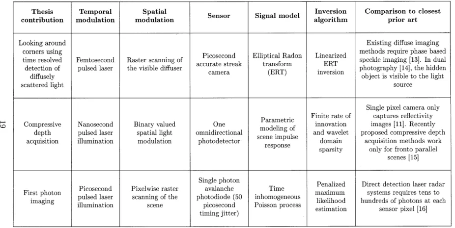
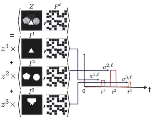
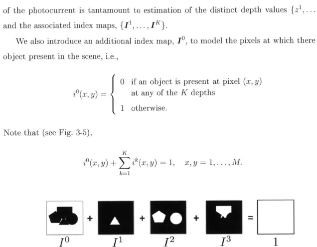
The imaging setups and problem statements for each of the above scenarios are shown and discussed in Figs. 1-3-1-5. A brief overview and comparison of thesis contributions is presented in Table 1.1. The rest of the thesis is organized into chapters corresponding to the aforementioned scenarios. Within each section we discuss:

1. Overview of the problem.

2. Prior art and comparison with proposed computational imager. 3. Imaging setup, data acquisition, and measurement models. 4. Novel image formation algorithms.

5. Experimental setup and results.

(16)

diffuse reflector diffuse light s occl occluded scene r femtosecond duration

raster scanned pulsed illumination

illumination I time

0

red time-varying

light source cene response

IT>

-non-spatially resolving,

0 time time-resolved sensor

uder

computational synchronization,

pr- esig - control and

data buffng

Figure 1 3: Looking around corners using ultrashort pulsed illumination and

picosecond-accurate time-sampling of diffusely scattered light: Here the goal is to reconstruct the position

and reflectivity of an object that is occluded from the light source and the sensor. We achieve this chal lenging task by raster scanning a diffuser with ultrashort pulsed illumination and by time sampling the backscattered light with picosecond accuracy. The computational processing of this time resolved data using elliptical Radon transform inversion reveals the hidden object's 3D position and reflectivity.

scene . ' nanosecond duration pulsed illumination spatial modulator time-varying

patterns light source

sceneresponses

non-sp atially resolving, time-r solved sensor

0 time

computationai synchronization, conatb and

<-proces ngdata _buffering

Figure 1 4: Compressive depth acquisition using structured random illumination and a single time-resolved sensor: Here, we are interested in compressively acquiring scene depth using structured

illumination and single time resolved sensor. This problem may seem analogous to the single pixel camera [11, 12], but unlike reflectivity, it is not possible to measure linear projections of scene depth. We solve this problem for planar and fronto parallel scenes using parametric signal modeling of the scene impulse response and using finite rate of innovation methods to reconstruct the scene's impulse responses using time resolved illumination and detection.

(17)

ambient

ght sub-nanosecond duration

raster scanned pulsed illumination

illumination ₃_time

0

time-varying

scene light source

response non-spatially resolving, single-photon counting Detector (SPAD) 0 time compuetwolsynchrmnization, Ingmputttooan 4-Processingthhrn

Figure 1 5: 3D and reflectivity imaging using one detected photon per pixel: Here, we are interested in reconstructing accurate 3D and reflectivity images of the scene using only one detected photon per pixel, even in the presence of strong background light. We achieve this using physically accurate modeling of single photon photodetection statistics and exploitation of spatial correlations present in real world scenes.

1.2 Key Publications

Most of the material presented in this thesis has previously appeared in the following pub-lications and manuscripts listed below:

Looking Around Corners or Hidden-Plane Imaging

1. A. Kirmani, A. Velten, T. Hutchison, M. E. Lawson, V. K. Goyal, M. G. Bawendi, and R. Raskar, Reconstructing an image on a hidden plane using ultrafast imaging of diffuse reflections, submitted, May 2011.

2. A. Kirmani, H. Jeelani, V. Montazerhodjat, and V. K. Goyal, Diffuse imaging: Creat-ing optical images with unfocused time-resolved illumination and sensCreat-ing, IEEE Signal Processing Letters, 19 (1), pp. 31-34, October 2011.

Compressive Depth Acquisition

1. A. Kirmani, A. Colago, F. N. C. Wong, and V. K. Goyal, Exploiting sparsity in

time-of-flight range acquisition using a single time-resolved sensor, Optics express 19 (22),

(18)

2. A. Colago, A. Kirmani, G. A. Howland, J. C. Howell, and V. K. Goyal, Compressive depth map acquisition using a single photon-counting detector: Parametric signal pro-cessing meets sparsity, In IEEE Conf. on Computer Vision and Pattern Recognition

(CVPR), pp. 96-102, June 2012.

Photon-efficient Active Optical Imaging

1. A. Kirmani, D. Venkatraman, D. Shin, A. Colago, F. N. C. Wong, J. H. Shapiro, and V. K. Goyal, First-Photon Imaging, Science 343 (6166), pp. 58-61, January 2014. 2. D. Shin, A. Kirmani, V. K. Goyal, and J. H. Shapiro, Photon-Efficient Computational

3D and Reflectivity Imaging with Single-Photon Detectors, arXiv preprint arXiv:1406.1761,

June 2014.

(19)

Thesis Temporal Spatial Sensor Signal model Inversion Comparison to closest

contribution modulation modulation algorithm prior art

Looking around Existing diffuse imaging

corners using Picosecond Elliptical Radon Linearized methods require phase based time resolved Femtosecond Raster scanning of accurate streak transform ERT speckle imaging [13]. In dual detection of pulsed laser the visible diffuser photography [14], the hidden

diffusely camera (ERT) object is visible to the light

scattered light source

Single pixel camera only . Finite rate of captures reflectivity Compressive Nanosecond Binary valued One Paaeic innovation images [11]. Recently

depth pulsed laser spatial light omnidirectional meng of and wavelet proposed compressive depth acquisition illumination modulation photodetector scene impulse domain acquisition methods work

response sparsity only for fronto parallel scenes [15]

Single photon _Penalized _{Direct detection laser radar} First photon Picosecond Pixelwise raster avalanche Time maximum systems requires tens to

imaging pulsed laser scanning of the photodiode (50 inhomogeneous likelihood hundreds of photons at each illumination scene picosecond Poisson process estimation sensor pixel [16]

timing jitter)

(20)

(21)

Chapter 2 Looking Around Corners

2.1 Overview

Conventional imaging involves direct line-of-sight light transport from the light source to the scene, and from the scene back to the camera sensor. Thus, opaque occlusions make it impossible to capture a conventional image or photograph of a hidden scene without the aid of a view mirror to provide aii alternate path for unoccluded light transport between the light source, scene and the sensor. Also, the image of the reflectivity pattern on scene surfaces is acquired by using a lens to focus the reflected light on a two-dimensional (2D) array of light sensors. If the mirror in the aforementioned looking around corners scenario was replaced with a Lambertian diffuser, such as a piece of white matte paper, then it becomes impossible to capture the image of the hidden-scene using a traditional light source and camera sensor. Lambertian scattering causes loss of the angle-of-incidence information and results in mixing of reflectivity information before it reaches the camera sensor. This mixing is irreversible using conventional optical imaging methods.

In this chapter we introduce a computational imager for constructing an image of a static hidden-plane that is completely occluded from both the light source and the camera, using only a Lambertian surface as a substitute for a view mirror. Our technique uses knowledge of the orientation and position of a hidden-plane relative to an unoccluded (visible) Lambertian diffuser, along with multiple short-pulsed illuminations of this visible diffuser and

(22)

time-k-. 14 cf T Hidden _S, Scene S4 14-

C

cm'a B s, Occluder Pulsed -10e Light D 2D

45* SurceCamera Pixel ndex

-21 'cm

2D-C

Time- Computational

resolved

4- _CIO _Cameraamr Reconstruction

Lambertian Diffuser

Figure 2-1: Looking around corners imaging setup for hidden-plane reflectivity construction.

resolved detection of the backscattered light, to computationally construct a black-and-white image of the hidden-plane.

The setup for looking around corners to image a static hidden-plane is shown in Fig. 2-1. A pulsed light source serially illuminates selected points, Si, on a static unoccluded Lamber-tian diffuser. As shown, light transport from the illumination source to the hidden-scene and back to the camera is indirect, possible only through scattering off the unoccluded Lamuber-tian diffuser. The light pulses undergo three diffuse reflections, diffuser -+ hidden-plane -*

diffuser, after which they return to a camera co-located alongside the light source. The opti-cal path differences introduced by the multipath propagation of the scattered light generates a time profile that contains the unknown hidden-plane reflectivity (the spade). A time-resolved camera that is focused at the visible diffuser and accurately time-synchronized with the light source time-samples the light incident from observable points on the diffuser, Dj.

Given the knowledge of the complete scene geometry, including the hidden-plane orientation and position, the time-sample data collected by interrogating several distinct source-detector pairs, (Si, Dj), is computationally processed using a linear inversion framework (see Figs. 2-2 and 2-8) to construct an image of the hidden-plane (see Fig. 2-9).

(23)

The remainder of this chapter is organized as follows. Prior art is discussed in Section 2.2. Then Section 2.3 introduces the imaging setup and signal model for the proposed looking around corners computational imager. Next, Section 2.4 presents the scene response model. The measurement model and data acquisition pipeline are described in Section 2.5. These models form the basis for the novel hidden-plane reflectivity estimation algorithm developed in Section 2.6. The experimental setup and results are presented in Section 2.7 and finally Section 2.8 provides additional discussion of limitations and extensions.

2.2 Prior Art and Challenge

Non line-of-sight imaging: Capturing images despite occlusions is a hard inverse imaging problem for which several methods have been proposed. Techniques that use whatever light passes through the occluder have been developed. With partial light transmission through the occluder, time-gated imaging [17,181 or the estimation and inversion of the mesoscopic transmission matrix [13] enables image formation. While some occluding materials, such as biological tissue, are sufficiently transmissive to allow light to pass through them [19,20], high scattering or absorption coefficients make image recovery extremely challenging. There are also numerous attempts to utilize light diffusely-scattered by tissue to reconstruct embedded objects [13, 21]. Our proposed computational imager is based on the pulsed illumination of the hidden-scene by reflecting off the visible diffuser followed by time-sampling of the backscattered light, rather than on transmission through the occluder itself. As opposed to prior work on non line-of-sight imaging [13,19 21] we image around the occluder rather than through it, by exploiting the finite speed of light.

Illumination wavelengths may be altered to facilitate imaging through occluders, as in X-ray tomography [22] or RADAR [23,24]. However, such imaging techniques do not yield

images in the visible spectrum that are readily interpreted by a human observer.

Hidden-scene image capture has been demonstrated, provided there is direct line-of-sight at least between the light source and the scene, when the scene is occluded with respect to the sensor

[14].

This was accomplished by raster scanning the scene by a light source followed by computational processing that exploits Helmholtz reciprocity of light transport.

(24)

Looking around corners using diffuse reflections: The closest precedent to the ineth-ods proposed in this chapter experirrientally demonstrated the recovery of hidden-scene struc-ture for one-dimensional scenes, entirely using diffusely-scattered light [25 27]. Selected visi-ble scene points were illuminated with directional short pulses of light using one-dimensional femtosecond laser scanning. The diffuse, scattered light was time-sampled using a single-pixel detector with picosecond resolution. The resulting two-dimensional dataset was pro-cessed to compute the time-delay information corresponding to the different patches in the hidden-scene. Then, standard triangulation algorithms were used to estimate the geomet-ric parameters of a simple occluded scene. The geometry reconstructions were noted to be highly susceptible to failure in the presence of noise and timing jitter. Also, the experimental validation of these methods was limited to a very simple one-dimensional scene comprising only three mirrors. While [25 27] used time-of-arrival measurements to enable estimation of hidden-scene geometry, estimation of hidden-scene reflectivity, which is also contained in the light signal, has not been accomplished previously.

Synthetic aperture radar: The central contribution in this chapter is to demonstrate the use of temporal information contained in the scattered light, in conjunction with appropriate post-measurement signal processing, to form images that could not have been captured using a traditional camera, which employs focusing optics but does not possess high temporal resolution. In this connection it is germane to compare our proposed computational imager to synthetic aperture radar (SAR), which is a well-known miicrowave approach for using time-domain information plus post-measurement signal processing to form high spatial-resolution images [28 30]. In stripmap mode, an airborne radar transmits a sequence of high-bandwidth pulses oi a fixed slant angle toward the ground. Pulse-compression reception of individual pulses provides across-track spatial resolution superior to that of the radar's antenna pattern as the range response of the compressed pulse sweeps across the ground plane. Coherent integration over many pulses provides along-track spatial resolution by forming a synthetic aperture whose diffraction limit is much smaller than that of the radar's antenna pattern.

SAR differs from the proposed computational imager in two general ways. First, SAR requires the radar to be in miotion to scan the scene, whereas the proposed imager does

(25)

not require sensor motion because it relies on raster scanning the beam on the visible dif-fuser. Second, SAR is primarily a microwave technique, and most real-world objects have a strongly specular bidirectional reflectance distribution function [31] (BRDF) at microwave wavelengths. With specular reflections, an object is directly visible only when the angle of il-lumination and angle of observation satisfy the law of reflection. Multiple reflections which are not accounted for in first-order SAR models can then be strong and create spurious im-ages. On the other hand, most objects are Lambertian at optical wavelengths, so our imager operating at near-infrared wavelengths avoids these sources of difficulty.

Time-resolved imaging of natural scenes: Traditional imaging involves illumination of the scene with a light source whose light output does not vary with time. The use of high-speed sensing in photography is associated with stopping motion [4]. In this thesis, we use time-resolved sensing differently: to differentiate among paths of different lengths from light source to scene to sensor. Thus, as in time-of-flight depth cameras [9,10] that are covered in detail in Chapter 3, we are exploiting the speed of light being finite. However, rather than using the duration of delay to infer distances, we use temporal variations in the backreflected light to infer scene reflectivity. This is achieved through a computational unmixing of the reflectivity information that is linearly combined at the sensor because distinct optical paths may have equal path lengths (see Fig. 2-2).

Some previous imagers, like light detection and ranging (LIDAR) [91, systems have em-ployed pulsed illumination and highly sensitive single-photon counting time-resolved detec-tors to more limited effect. Elapsed time from the pulsed illumination to the backreflected light is proportional to target distance and is measured by constructing a histogram of the photon-detection times. The operation of LIDAR systems is discussed in detail in Chapter 5. In the context of LIDAR systems, time-based range gating has been used to reject unwanted direct reflections in favor of the later-arriving light from the desired scene [32 341. Captur-ing multiple such time-gated images allows for construction of a three-dimensional model of the scene [17,181, as well as for imaging through dense scattering media, such as fog or foliage

[33,351.

As opposed to the methods proposed in this chapter, however, the aforemen-tioned LIDAR-based techniques also rely on using temporal gating to separate the direct,

(26)

unscattered component of the backreflected light from the diffusely-scattered component.

Challenge in Hidden-Plane Image Formation

To illustrate the challenge in recovering the reflectivity pattern on the hidden-scene using only the backscattered diffuse light, we pick three sample points A, B, and C on the hidden-plane. Suppose we illuminate the point S1 on the visible Lambertiani diffuser with a very short laser pulse (Fig. 2-2A), and assume that this laser impulse is scattered uniformly in a hemisphere around S1 and propagates toward the hidden-plane (Fig. 2-2B). Since the hidden points A, B, and C may be at different distances from Si, the scattered light reaches them at different times. The light incident at A,B and C undergoes a second Lambertian scattering and travels back towards the visible diffuser with attenuations that are directly proportional to the unknown reflectivity values at these points (see Fig. 2-2C).

The visible diffuser is in sharp focus of the camera optics, so each sensor pixel is observing a unique point on the diffuser. We pick a sample point D1 that functions as a bucket detector

collecting backscattered light from the hidden-plane without angular (directional) sensitivity and reflecting a portion of it towards the camera. The hidden points A, B, and C may be at different distances from D1 as well. Hence, light scattered from these points reaches the

camera at different times. The times-of-arrival of the light corresponding to the distinct optical paths, light source-* S -4(A, B, C)-+ D1 -+camnera, depend on the scene geometry

(see Fig. 2-2D), which we assume to be known.

Diffuse scattering makes it impossible to recover the hidden-plane reflectivity using tradi-tional optical imaging. An ordinary camera with poor temporal resolution records an image using an exposure time that is at least several microseconds long. All of the scattered light, which includes the distinct optical paths corresponding to A, B, and C, arrives at the sensor pixel observing D1 during this exposure time and is summed into a single intensity value

(see Fig. 2-2E), making it impossible to recover the hidden-plane reflectivity.

We now discuss how temporal sampling of the backscattered light allows at least partial recovery of hidden-plane reflectivity. Suppose now that the camera observing the scattered light is precisely tirme-synchronized with the outgoing laser pulse, and possesses a very high

(27)

A

Hidden Hidden

Scene Scene

B

Occluder Light _Occluder _Light

Source Source

t=5 t=1

Lambertlan Camera Lambertian Camera

Diffuser Diffuser

CHiden

D

Hdden

Scene Scene

t=8 B

tt=8

8

Occluder LgtOccluderLih

~LightLgh

Source Source

t=9

Lambertian Camera Lambertian Camera

Diffuser Diffuser t 12 t = 12t 13 t 13

E

100F

AC

TTm

0 0 (picoseconds) Pixe

Pixel Index - Index

Figure 2-2: Challenge in hidden-plane image formation. (A)-(D) Time-dependent light transport

diagrams showing diffuse scattering of the short pulse illumination through the imaging setup and back to the camera. The hidden point B has the shortest total path

length,

S1 -+ B -+ D1, and the points A and C have equal total path

lengths.

(E) An ordinary camera with microsecond long exposure integrates the entire scattered light time profile into a single pixel value that is proportional to the sum of all hidden plane reflectivity values. (F) Exploiting the differences in total path

lengths

allows partial recovery of hidden plane reflectivity. For example, reflectivity at B is easily distinguishable from that at points A and C via temporal sampling of the scattered light. Several points

on

the hidden plane, such as A and C, have equal total path

lengths

and even using a time resolved camera, we may only record a sum of their reflectivity values. timse-sampling resolutioni. As shown ini Fig. 2-2(F), the measured time-samples can

(28)

may be multiple points on the hidden-plane such that the light rays corresponding to these points have equal optical path lengths and therefore have the same time-of-arrival at the camera sensor. We call this phenomena mnultipath mixing: the summation of the hidden-plane reflectivity information due to equal total optical path lengths. Although undesirable, this mixing is reversible.

As described in Section 2.4, the hidden-plane reflectivity values that are added together belong to a small set of points on the hidden-plane that lie within a known elliptical shell. As shown in Section 2.6, spatio-temporal sampling followed by a linear inversion allows the complete recovery of hidden-plane reflectivity from time-resolved measurements.

2.3 Imaging Setup

Our imaging setup (see Fig. 2-1) comprises a pulsed collimated light source serving as our directional illumination source which is co-located with a resolved camera that time-samples the backscattered light. The hidden-scene consists of a single occluded hidden-plane composed of Lambertian material with an unknown reflectivity pattern. We assume that the 3D orientation, position and dimensions of the hidden-plane areknown a priori. If these geometric quantities are unknown, then they may be first estimated using the hidden-plane geometry estimation method described in [25 27]. We also assume that the reflectivity pattern, 3D position, and orientation of the visible Lambertian diffuser relative to the cam-era and light source are known. These quantities can be easily estimated using traditional imaging techniques. The complete knowledge of 3D scene geometry allows us to formu-late hidden-plane reflectivity estimation as a linear inversion problem. This formulation is described next, but we first make a sinmplification.

Simplified illumination and sensing model: In our data acquisition setup the points of interest on the visible diffuser, {Sj}_1, are illuminated one at a time with a collimated beam of pulsed light. Since the visible diffuser is assumed to be perfectly Lambertian, it scatters the incident light uniformly in all directions. We assume that at least a part of this scattered light illuminates the entire hidden-plane for each {Sj}_1. Given this assumption,

(29)

it is possible to abstract the combination of the pulsed light source and the chosen visible diffuser points, {Si}, into six omnidirectional pulsed light sources whose illumination profiles are computed using the surface normal at these points, the angle of incidence of the collimated beam and the reflectivity at these points.

Similarly, each ray of backreflected light from the hidden-plane is incident at the visible diffuser points, {Dj}i, where it undergoes another Lambertian scattering and a portion of this scattered light reaches the time-resolved camera optics. The points, {Dj}>_1, are in sharp focus relative to the time-resolved camera, which comprises of a horizontally oriented, linear array of sensors that time-sample the incident light profile relative to the transmitted laser pulse. Since all the orientations, distances and dimensions of the scene are assumed to be known, it is possible to abstract the combination of the time-resolved camera and the chosen visible diffuser points, {Dj}, into three resolved bucket detectors that are time-synchronized with the omnidirectional light sources {Sj}_1. The sensitivity profiles of these

bucket detectors are known functions of the reflectivity and surface normals at these points, and their orientation relative to the hidden-plane that determines the angle of incidence of backscattered light.

In order to further simplify our mathematical notation, we assume that each of the omnidirectional light sources, {Si}i_ 1, transmits equal light power in all directions and that

each of the bucket detectors, {Dj}>1, has a uniform angular sensitivity profile.

In effect, as shown in Fig. 2-3, we abstract the entire hidden plane imaging setup into a set of six omnidirectional pulsed light sources illuminating the hidden-plane with a common pulse shape s(t), and three tine-resolved bucket detectors with a common impulse response h(t) that time-sample the backscattered light with sampling interval, T,. The 3D positions of the (source, detector) pairs {Si, Dj}Q i- are known and they are assumed to be accurately time-synchronized to enable time-of-arrival measurements. We also assume that there is no background light and that the imager operates at single wavelength.

Hidden-plane scene setup: We have assumed that the position, orientation, and dimen-sions (W-by-W) of the hidden Lambertian plane are known or estimated a priori. Formation of an ideal grayscale image therefore is tantamount to the recovery of the reflectivity pattern

(30)

visible diffuser B hidden Scene S6 S S4 S3 i D w- hidden Scene s S4 e 0 D s, se omni-directional light sources i bucket detectors

Figure 2 3: Simplified illumination and detection model. (left) Portion of the hidden plane imaging setup in Fig. 2 1 comprising the visible diffuser, the hidden plane, and the chosen points of illumination and detection. (right) The simplified imaging setup, under the assumptions stated in Section 2.3, is equivalent to the setup in the left sub figure.

on the hidden-plane. As is usual in optics and photometry, reflectivity is defined as the fraction of incident radiation reflected by a surface. Reflectivity is thus bounded between 0 and 1. Therefore, in this chapter, hidden-plane reflectivity is modeled as a 2D function a : [0, W]2

-* [0,1]. In general, the surface reflectivity must be treated as a directional

property that is a function of the reflected direction, the incident direction, and the incident wavelength [361. We assume, however, that the hidden-plane is Lambertian, so that its per-ceived brightness is invariant to the angle of observation [311; incorporation of any known

BRDF would not add insight.

2.4 Scene Response Modeling

The backreflected light incident at sensor Dj in response to hidden-scene illumination by source Si is a combination of the tie-delayed reflections from all points on the hidden-plane. For any point x = (x, y) E [0, WI2, let zs(x) denote the distance from illumination source Si

to x, and let zf(x) denote the distance from x to sensor Dj. Then zfD(X) = (X) + zfX)

30

(31)

0.s5

Se

D2 45cm

(a) source S6 and sensor D2

0.5

45 cm

30 m

(b) source S2 and sensor D

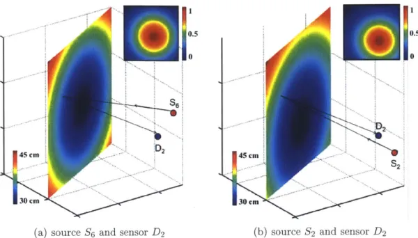
Figure 2 4: Main plots: Time delay from source to scene to sensor is a continuous function, zSD (x), of the

32

position in the scene. The range of zSD

(x)

values shown in this figure corresponds to the scene geometry in

Fig. 2 1. Insets: The normalized geometric attenuation aij(x) of the light is also a continuous function of the position in the scene (see Equation (2.1)).

is the total distance traveled by the contribution from x. This contribution is attenuated by the reflectivity a(x), square-law radial fall-off, and cos(0(x)) to account for foreshortening of the hidden-plane with respect to the illumination, where 0(x) is the angle between the surface normal at x and a vector from x to the illumination source. Thus, the backreflected waveform from the hidden-scene point x is

ai (x) a(x) s(t - zjD(X)/c),

where c is the speed of light and

ap

(X) cos(0(x))

z (x) zP (x))

(2.1)

Examples of distance functions and geometric attenuation factors are shown in Figure 2-4. Combining contributions over the plane, the total light incident at detector Dj in response to hidden-scene illumination by source Si is,

(32)

w w

rij(t)

JJ

(x) a(x) s(t - z D (x)/c) dx dy.

0 0 W W~

[I

ajj(x) a(x) (t - z D(x)/c) dxddy *s(t).

where * denotes continuous-time convolution, 6(.) is the Dirac delta function, and equality ( follows from the Dirac sifting property.

Putting aside for now the effect of the pulse waveform, s(t), we define the scene impulse response function corresponding to the (source, detector) pair, (Si, Dj), as

pij (t) - ajj(x) a(x) 6(t - zSj (x)/c) dx dy. (2.2)

0 0

Thus, evaluating pij(t) at a fixed time t amounts to integrating over x E [0, W]2 _with

t zsjD(x)/c. Define the isochronal curve Ci = {x : z D(X) = ct}. Then

pij(t) Jaij(x)a(x) ds aij (x(k, u))a(x(k, u)) du dk (2.3)

Ct

where x(k, u) is a parameterization ofcjj

n

[0, W]2_{. The scene impulse response pij(t) thus} contains the contour integrals over Cli's of the desired function a. Each Cjj is a level curve

of zsD(x); as illustrated in Figure 2-4, these are ellipses.

2.5 Measurement Model

A digital system can use only samples of rij(t) rather than the continuous-tine function itself. We now show how uniform sampling of rij(t) with a linear time-invariant (LTI) prefilter relates to linear functional measurements of a. This establishes the foundation for a Hilbert space view of our computational imaging formulation.

(33)

At the detector the backreflected light signal, rij(t), is convolved with the sensor impulse response filter, h(t), prior to discrete time-sampling with a sampling interval T, in order to produce time-samples denoted,

ri [n]

=

(rij

(t) *

h(t))

T,

The sample data length, N, is chosen sufficiently high so that NT, is slightly greater than the time-domain support of the signal rij(t). Also, in this chapter we use the box-detector impulse response to match the operation of the streak camera that was employed in our experimental setup in Section 2-7, i.e.,

h(t) =

1,

10,)

for 0 < t < T,;

otherwise,

corresponding to integrate-and-dump sampling in which the continuous signal value is first integrated for duration T, and sampled immediately thereafter. Also, note that by the

associativity of the convolution operator,

rij [n] = (pij(t) * s(t) * h(t)) t=, T

Defining the combined impulse response of the source-detector pair, g(t) - s(t) * h(t), we

obtain

r-i [n] = _{(pij (t) * g(t))}_tnT,

A time-sample rij[n] can be seen as a standard 2(R) inner product between pij(t) and a time-reversed and shifted system impulse response, g(t) [37], i.e.,

ri [n] = (pij (t), g(nT. - t)). (2.5)

Using Equation (2.2), we can express Equation (2.5) in terms of a using the standard

(2.4)

n = 0, 1, . . ., (N - 1).

(34)

2([0, W]2) inner product:

rij[n] = (a, pi~j,n) where (2.6)

pij,n(x) = aij(x) g(nT, - zD (x)/c). (2.7)

Over a set of sensors and sample times, {ij,n} will span a subspace of L2([O, W]2), and a sensible goal is to form a good approximation of a in that subspace.

Now, since h(t) is nonzero only for t C [0, T], by Equation (2.5), the time-sample rij[n] is the integral of rij (t) over t E [(n-1)T, nTI. Thus, by Equation (2.3), rij[n] is an aij-weighted integral of a between the contours C (l)T, and CTs. To interpret this as an inner product with a, as in Equations (2.6) and (2.7), we note that Pi,,(x) is aij(x) between C> and CT and zero otherwise. Figure 2-5(a) shows a single representative pij,n. For the case of the box-detector impulse response (see Equation (2.4)), the functions { i,,}nEZ for a single sensor have disjoint supports; their partitioning of the domain [0, W]2

is illustrated

in Figure 2-5(b).

Data acquisition: For each time-synchronized source-detector pair, (Si, Dj), N discrete time-samples were collected as follows: the light sources were turned on one at a time, and for each light source all the detectors were time-sampled simultaneously. The use of the resulting dataset, {rij[n]} i= 3 --1, in recovering the hidden-scene reflectivity, a, is

described next.

2.6 Image Recovery using Linear Backprojection

Piecewise-constant Model for Hidden Plane Reflectivity

To express an estimate a of the reflectivity a, it is convenient to fix an orthonormal basis for a subspace of 2([0, W]2) and estimate the expansion coefficients in that basis. For an

(35)

0.5 0

30 cm

(a) source S6 and sensor D2

M

b

cm

(b) source S2 and sensor D2

Figure 2 5: (a) A single measurement function Pi,jn(x) when h(t) is the box function defined in Equa tion (2.4). Inset is unchanged from Figure 2 4(a). (b) When h(t) is the box function defined in Equa tion (2.4), the measurement functions for a single sensor {pijn(x)}N_1 partition the plane into elliptical annuli. Coloring is by discretized delay using the colormap of Figure 2 4. Also overlaid is the discretization of the plane of interest into an M by M pixel array.

M-by-M pixel representation, let

M/W,

for (mx

-

1)W/M

< x < mxW/M,

bmx,my(x)

(mY

- 1)W/M < y < mYW/M;

0, otherwise

m, my= .1, ... M (2.8)

so that the hidden-plane reflectivity estimate has the following representation

M M

a

=:

&O(mX,

_{my) mXmy,}

m =1 mY=1

(2.9)

which lies in the span of the vector space generated by the orthonorial basis vector collection,

{'Cmmm C L2([0, W]2)xm IM , =M

(36)

Linear System Formulation of Measurement Model

We will now form a system of linear equations to find the basis representation coefficients {&V(mx, m,)}2-M!""M. For & to be consistent with the value measured by the detector Dj in response to hidden scene illumination by source Sj at time t = nT, we must have

M M

rij [n] = ( ,n,) = E E &0 (mnx, My) (Orm,mny , Oij,n). (2.10)

mn=1 my=l

Note that the inner products { (mx,my, Pi,n)} exclusively depend on M, W, the positions of illumination sources and detectors, {S,, Dj}i i, the hidden-plane geometry, the combined source-detector impulse response g(t), and the sampling intervals T, not on the unknown reflectivity of interest a. Hence, we have a system of linear equations to solve for the basis coefficients &p (mX, my). (In the case of orthonormal basis defined in Equation (2.8), these coefficients are the pixel values multiplied by M/W.)

When we specialize to the box sensor impulse response defined in Equation (2.4) and the orthonormal basis defined in Equation (2.8), many inner products (4mx,my, Oi,j,n) are zero, so the linear system is sparse. The inner product (4mX,my, ij,n) is nonzero when the reflection from the pixel (mr, my) affects the light intensity at detector Dj in response to hidden-plane illumination by light source Si within tine interval [(n - 1)T, nT]. Thus, for a nonzero inner product the pixel (mx, my) must intersect the elliptical annulus between C"-'T and CnS. With reference to Figure 2-5(a), this occurs for a small fraction of (mr, my) pairs unless M is small or T, is large. The value of a nonzero inner product depends on the fraction of the square pixel that overlaps with the elliptical annulus and the geometric attenuation factor.

To express Equation (2.10) as a vector-inatrix multiplication, we replace double indices with single indices (i.e., vectorize, or reshape) to get

y = E &' (2.11)

where y E Rl8xN contains the data samples

{rij[n]},

the first N from source-detector pair (S1, D1), the next N from source-detector pair (S1, D2), etc.; and &, R R 2

con-tains the coefficients &V,(m2, my), varying i first and then j. Then the inner product

(37)

1 M2

0

Figure 2 6: Visualizing linear system representation

E

in (2.11). Contribution from source detector pair (SI, D1) is shown. To generate this system matrix we choose M = 10 and therefore the

E

has 100

columns. Also we choose T, such that

E

has 40 rows. All zero rows arising from times prior to first arrival of light and after the last arrival of light are omitted.

(OmX,my, SPij,n) appears in row ((i - 1) x 6 + (j - 1) x 3)N + n, and column (mx - _1)M+ my

of

E

E R18xNxM2. Figure 2-6 illustrates an example of the portion of 0 corresponding to source-detector pair (S1, D1) for the scene in Figure 2-3.

Assuming that

E

has a left inverse (i.e., rank(e) = M2

), one can form an image by solving Equation (2.11). The portion of

E

from one source-detector pair cannot have full column rank, because of the collapse of information along elliptical annuli depicted in Fig-ure 2-5(a). Full rank and good matrix conditioning [38] are achieved with an adequate number of source-detector pairs, noting that such pairs must differ significantly in their spa-tial locations to increase rank and improve conditioning. As a rule of thumb, greater spaspa-tial disparity between (source,detector) pair positions improves the conditioning of the inverse problem. In this chapter, we use 18 well-separated (source, detector) pairs to satisfy the full-rank condition and to achieve good matrix conditioning.

Hidden-Plane Reflectivity Estimation

The unconstrained least-squares estimate for the hidden-plane reflectivity under the piecewise planar reflectivity model is [38]:

(38)

The M x M pixel image is obtained after reshaping the solution vector back to al array. Since reflectivity is constrained to lie within the interval [0, 1], the constrained least-squares estimate that satisfies this bounded reflectivity condition is obtained by the pixelwise thresh-olding of the unconstrained reflectivity estimate [38], i.e.,

for dULS(m,, my) > 1;

&LS (mx, my) 0 , for dULS(mx, my) < 0; m, m = 1,... , M dULS(mnx, my), otherwise.

Mitigating the effect of measurement noise: We assume that the time samples, ri[n], are corrupted with signal-independent, zero-mean, white Gaussian noise of a known variance,

72, which depends on the choice of the detector and time-sampling assembly.

We employ two main methods to reduce the effect of noise: First we reduced noise in the time-samples by repeatedly illuminating the static scene and averaging the measured tie-samples. Second, we employed constrained Tikhonov regularization [38] to obtain the following hidden-plane reflectivity estimate,

1

for iU-TIKH

6ZC-TIKH(rn, mY) 0 , for &U-TIKH(mT, my) 0; m my y, - 1, - - M

ZU-TIKH(Mx, Tym), otherwise,

(2.12)

where

-U-TIKH _ _)T' ₊ _4T) _-1 _OTy,

<D is the discrete wavelet transform (DWT) matrix derived from Daubechies's 2-tap filter [39]

(1i, -1]/N2), and

#

- [0, 1] is a weight parameter to control the degree of Tikhonov regular-ization. A high value of the weight parameter, 0, forces the reflectivity image to be overly smooth while a low-value of

#

leads to noisy reflectivity estimates. Therefore, an optimal value of

#

needs to be chosen. In this chapter, we selected this optimal /-value by con-structing the reflectivity image for

#

= {0.1, 0.2, . . ., 0.9} and then choosing the one which minimized the squared error 11y -

e

&UTIKH

Computational time-resolved imaging

Computational Time-resolved Imaging

by

Ghulam A. Kirmani

S.M., Media Technology

Massachusetts Institute of Technology, 2010

Integrated M.Tech in Mathematics and Computing

ARCHNE

MAR 19

2015

LIBRARIES

Indian Institute of Technology Delhi, 2008

Submitted to the

Department of Electrical Engineering and Computer Science

in partial fulfillment of the requirements for the degree of

Doctor of Philosophy in Electrical Engineering and Computer Science

at the

MASSACHUSETTS INSTITUTE OF TECHNOLOGY

February 2015

Massachusetts Institute of Technology 2015. All rights reserved.

Signature redacted

A u th or ...

...

Department of Electrical EngineerFig and Computer Science

Certified by

Signature redacted

mber 15, 2014

Certified by

Jeffrey H. Shapiro

Julius A. Stratton Professor of Electrical Engineering

Massachusetts Institute of Technology

j

/,,

Th'iis

Supervisor

Vivek

K

Goyal

Assistant Professor of Electrical and Computer Engineering

Boston University

A ccepted by ...

-

. t, . , .

. Thesis Supervisor

Signature redacted...

I'

sl'i4 A. Kolodziejski

Chair, Department Committee on Graduate Students

Computational Time-resolved Imaging

by

Ghulam A. Kirmani

Abstract

Acknowledgments

Contents

Chapter 1

Introduction

1.1

Summary of Main Contributions

IT>

1.2

Key Publications

Looking Around Corners or Hidden-Plane Imaging

Compressive Depth Acquisition

Photon-efficient Active Optical Imaging

Chapter 2

Looking Around Corners

2.1

Overview

C

2.2

Prior Art and Challenge

[14].

[33,351.

Challenge in Hidden-Plane Image Formation

A

CHiden

D

Hdden

8

~LightLgh