Cement Bond Evaluation Using Early Refracted Arrivals

(1)

REFRACTED ARRIVALS

Rama Rao V. N.

Earth Resources Laboratory

Department of Earth, Atmospheric, and Planetary Sciences Massachusetts Institu~eof Technology

Cambridge, MA 02139

Batakrishna MandaI

Halliburton Energy Services

Houston, TX

Arthur C. H. Cheng

Western Atlas Logging Services

Houston, TX and

Dept. of Earth, Atmospheric, and Planetary Sciences Massachusetts Institute of Technology

Cambridge, MA 02139

M. N afi Toksoz

Department of Earth, Atmospheric, and Planetary Sciences Massachusetts Institute of Technology

(2)

ABSTRACT

The cement bond evaluation tool is a device used to examine the integrity of cement bonding to the casing. A conceptual tool operating between 80-200 kHz is considered here, with a transmitter and two receivers, oriented parallel to the axis of the bore-hole and next to the casing. The compressional head wave in the casing, excited by the transmitter, will be the first arrival to be measured by the two receivers in most situations. With both receivers on the same side of the transmitter, the attenuation of this wave in traveling between the two receivers is dependent on the properties of the medium immediately outside the casing. The radially layered borehole was modeled as a layered plane medium for large operating frequency. A spectral integral approach (com-plete wave synthesis) was used to compute the response at the receiver locations, which then provided attenuations. Different parameters, such as transducer separation (1-12 in), annulus thickness (0-6 in), annulus impedance (free pipe to good cement), casing thickness (0.25-0.45 in), standoff distance (0.5-1 in) and source frequency (80-200 kHz) were varied in the evaluation of the operation of the tool. The parameter studies based on the theoretical computations revealed that free pipe could be distinguished from the presence of cement in a variety of situations. Additionally, lower bounds on receiver separations are given for reliable operation of the tool.

INTRODUCTION

Cement bond evaluation tools attempt to identify the presence of cement behind the casings using transmitters and receivers inside the casing. Cement bond logs have been used in the oil industry for more than three decades using sonic frequency (e.g., Walker, 1962, 1968; Pardue, et aI., 1963; Gollwitzer and Masson, 1982) and for more than a decade using ultrasonic frequency (e.g., Froelich, et aI., 1981; Havira, 1982). In this paper, we conduct numerical computations to evaluate the effect of different parameters of cement bonding to the casing.

The tool considered here is operating at ultrasonic frequency, and has a transmitter and two receivers that are parallel to the axis of the borehole and that are next to the casing. The two receivers are on the same side of the transmitter and the separation between the transmitter and the closest receiver is the same as that between the two receivers. The ratio of the earliest arrival at the two receivers is used to determine the attenuation of this wave traveling between the two receivers. Since it is a ratio of two response measurements, it is independent of the source power. This attenuation varies with the thickness and material properties of the casing, the cement and the formation. The sensitivity of the attenuation of the earliest arrival to layers outside the casing is used in characterizing the nature of the bond between the casing and the cement.

(3)

MODEL

The wavetypes that are recorded at the receivers include early refracted arrivals (com-pressional and shear), a reflected mud arrival and a direct (Stoneley) arrival. The arrival of concern is the refracted compressional arrival that impinges on the casing wall at near critical angles and travels along the casing wall as a compressional lateral wave in the steel and then radiates at near critical angles in a conical wavefront to the receivers COberall, 1973 ).

The operation of the tool is evaluated by computing the attenuation predicted by a model of the tool. The variation in the attenuation of the first arrival in traveling between the two receivers is examined as various model parameters are varied. This is used to elicit bounds of operation and sensitivity levels of the tool.

Assumptions

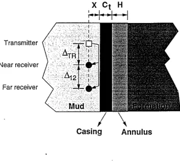
• The cylindrically layered borehole was modeled with plane layers. The typical op-erating frequencies of such tools are around 100 kHz. At such high frequencies the radial curvature of the borehole can be neglected. Hence, the offset-independent, horizontally stratified, seismo-acoustic model, OASES (Schmidt and Tango, 1986), was used to compute the effects of wave propagation between the source and re-ceiver. The model is shown in Figure 1. There are two plane layers, the casing and the cement, which are bound by two half spaces, the drilling mud on one side and the formation on the other.

• All media were modeled as being lossless. The attenuation of the first arrival is due to radiation into the formation and mud and due to spreading between the two receivers. The radiation to the formation depends on the coupling between the casing and the formation provided by the annulus material.

PARAMETER VARIATION

The attenuation is computed as the following parameters are varied.

1. Source frequency, Ricker wavelets with center frequencies from 80-200 kHz in steps of 20 kHz.

2. Annulus material properties, considering air, water, and weak and strong cement (the terms weak and strong cement are used specifically to indicate cement types with P impedances of 3 x 106 _{and 6 x 10}6 _kg/m2_{s, respectively).}

3. Annulus thickness, h, in the range 0.1-6 in. 4. Casing thicknesses, Ct, of 0.25, 0.35 and 0.45 in.

(4)

6. Standoff distances, X, of 0.5 and 1 in.

As the parameters are varied, the receiver responses for a wideband impulse is pre-dicted using OASES. This result is then bandpass-filtered for Ricker source wavelets of different center frequencies. The ratio of amplitudes of the first arrival at the two receivers is then computed to arrive at the apparent attenuation of the compressional head wave in traveling between the two receivers. In all attenuation plots, computed re-sults are marked with 'o's or '+'s, with a least squares fit solid line drawn through them. The attenuation corresponding to the 80 kHz Ricker source wavelet is plotted as a thick grey line and the attenuations of the six subsequent center frequencies are plotted as thin black lines. Increasing the center frequencies leads to increased attenuations, with

the 200 kHz response being the most attenuated. Also included are results for different annulus thickness and the media. The material properties used in the simulations are given in Table 1.

Casing Thickness Effects

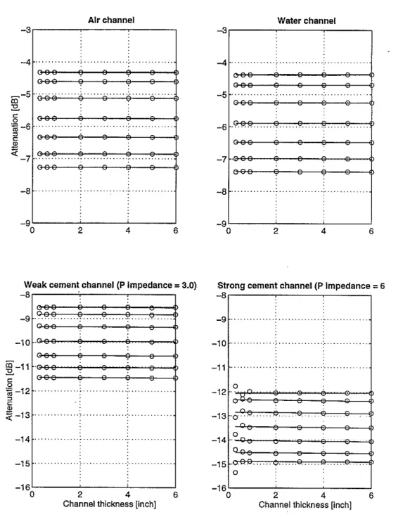
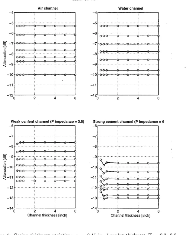
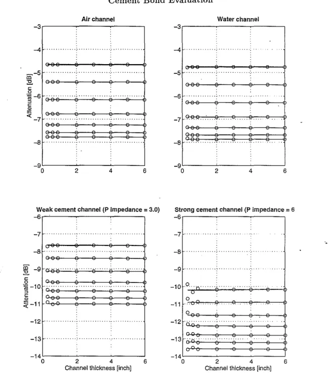
The attenuations are computed from the time responses at the two receivers for various annulus and casing thicknesses and are shown in Figures 2, 3 and 4. They show the computed first arrival attenuations for 0.25, 0.35 and 0.45 in thick casings, respectively. For most cases, attenuations are insensitive to annulus thickness greater than 1 in. As expected, the attenuations in cement are greater than that in air or water as there is stronger coupling and more efficient energy leakage into the formation. Attenuations in air and water increase with increasing casing thickness. However, this change is 1 dB at 80 kHz and 3 dB at 200 kHz. Thus, a more consistent performance in different casings can be expected at lower frequencies. The change in attenuation is a function of the change in the ratio of casing thickness to compressional wavelength in the casing, which is smaller for lower frequencies.

In weak cement, attenuations decrease as casing thickness changes from 0.25 to 0.35 in and then increase as it changes from 0.35 to 0.45 in. In contrast, strong cement attenuations decrease with increasing casing thickness. The attenuations are the result of the interaction of the casing, cement and formation, and exhibit undulations for different casing thicknesses and different layer properties.

Transducer Separation Effects

The transmitter-near receiver separation(b.rTR) and the near receiver-far receiver sep-aration (b.r12) are assumed to be the same. The term 'transducer separation' refers to the numerical value of both separations. The attenuations for different transmitter receiver separations are analyzed in two ways.

First, two transducer separations of 3 and 6 in are considered for a range of an-nulus thicknesses (0.1-6 in) when the anan-nulus medium is strong cement. This gives a highly resolved attenuation profile with annulus thickness, as shown in Figure 5. The

(5)

(1)

attenuations for 80 and 100 kHz at 3 in separation are not plotted due to the diffi-culty in identifying the amplitude of the first arrival. The profile of attenuation with annulus thickness exhibits variations at small annulus thicknesses, which levels out for thicknesses greater than 1 in.

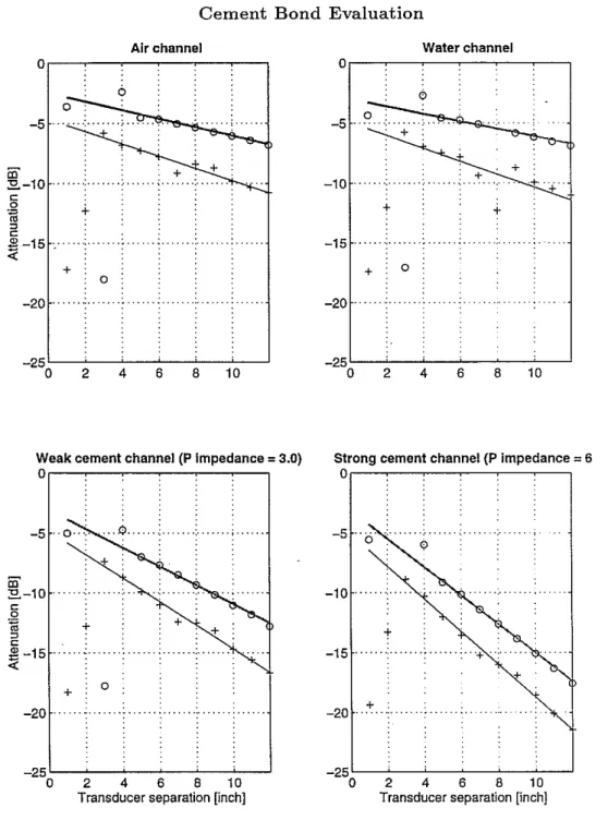
In the second case, the attenuations for a range of transducer separations, 1-12 in, are calculated for two specific annulus thicknesses, 0.5 and 1 in. Here, four different types of annulus media are considered. The attenuation profiles for 80 and 200 kHz alone are plotted for an annulus thickness of 0.5 in in Figure 6, and for 1 in in Figure 7. Attenuation increases linearly with transducer separation. Furthermore, the increase in attenuation with transducer separation is low for air and water (0.35 dB per in change of separation) compared to weak cement (0.7 dB/in) and strong cement (1.25 dB/in).

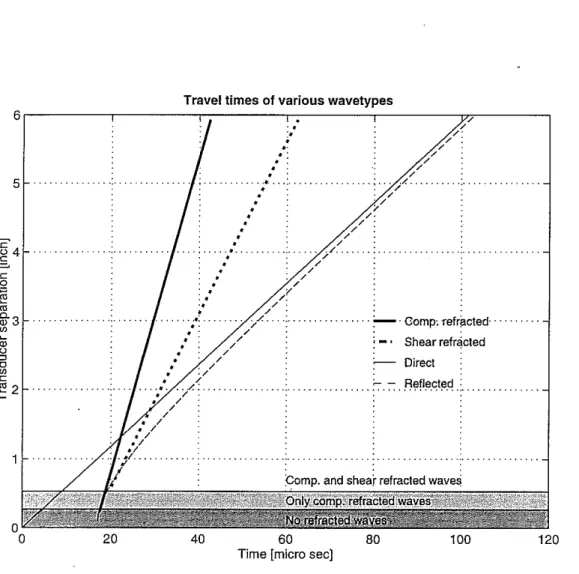
The erratic results for small separations are explained below. Figure 8 shows a plot of traveltimes of the various wavetypes in traveling from the source to the near receiver for different separations. This plot shows that at transmitter-near receiver separations

(6rTR) less than 1.30 in, the direct arrival (thin solid line) is the first arrival at the near receiver, while at larger separations it is the compressional refracted arrival (thick solid

line). The threshold separation is given by equating the traveltimes of the two paths.

6r 6r - -2Xtan

e,,12

2X

- =

+---,--" ' 1 ' "'2 "'1cos

e"

12

where

e,,12

is the compressional critical angle between the mud and the steel casing. Further, below 0.26 in separation, there are no refracted waves. Between 0.26 and 0.53 in only compressional refracted arrivals are present and above 0.53 in both refracted wavetypes are present. This is indicated in Figure 8 as different shaded regions. Thus at small separations, both receivers do not consistently measure the same wavetype in the first arrival. This accounts for the erratic attenuation profile in Figures 6 and 7. While a minimum transmitter-near receiver separation of 1.3 inches ensures that the compression arrival is the first arrival at both receivers, larger separations are required to ensure that the overlap with succeeding arrivals is minimized. Thus the attenuation estimates become consistent beyond a separation of 4 in at 80 kHz and 3 in at 200 kHz. This can also be seen as those transducer separations beyond which the leading arrival is separated from the next arrival by a time separation greater than the width of the Ricker wavelet (about 12 /.LS for 80 kHz and 5/.LS for 200 kHz).

Stand-Off Distance Effects

The attenuations for two different stand-off distances are calculated and plotted in Figures 9 and 10, with the results for 0.5 and 1 in stand-off distances, respectively.

With all parameters being the same, a change in stand-off distance from 0.5 to 1 in produces no change in attenuation levels. Moving all transducers away from the casing simultaneously changes the signal strength that they measure, but does not change their relative strengths. In this theoretical experiment, we assumed the same standoff distances for the transmitter and receivers.

(6)

CONCLUSIONS

A theoretical parametric study of the operating ranges of a cement bond evaluation tool was conducted over a wide range of parameters using frequency-wavenumber integration techniques, with the following results.

• Attenuation levels in free pipe (air and water in the annulus) are at least 2 dB lower than those in poor to good cement (weak and strong cement) in a wide variety of situations. Thus the presence or absence of cement can be detected with a tool of the type discussed here.

• Attenuation in weak cement is at least 2 dB less than that in the strong cement considered here. Thus it is possible to distinguish the quality of cement bond using this tool.

• Transducer separations, t:.TTR, need to be greater than 4 inches when operating at 80 kHz, and 3 inches, when operating at 200 kHz, to produce reliable attenuation results.

• Casing thickness changes the measured attenuation with the change being a func-tion of frequency. The lower source frequencies tend to be insensitive to casing thicknesses and produce consistent attenuation in different casings.

• Increasing transducer separations lead to increased attenuations with the increase being proportional to the impedance of the annulus material.

• Changes in standoff distance do not affect the attenuation profiles.

ACKNOWLEDGMENTS

This work was supported by the Borehole Acoustics and Logging Consortium at the Massachusetts Institute of Technology and by the Gas Research Institute, Chicago.

(7)

REFERENCES

Froelich, B., Dumont, A., Pittman, D., Seeman, 1981, B., and Ravira, M.,1981, Ultra-sonic imaging of material mechanical properties through steel pipe,IEEE Ultrasonics Symposium.

Gollitzer, L. R., and Masson, J. P., 1982, The cement bond tool, SPWLA Annual Logging Symposium.

Ravira, R. M., 1982, Ultrasonic cement bond evaluation, SPWLA Annual Logging Sym-posium, Corpus Christi, TX.

Pardue, G. R., Morris, R. L. Gollwitzer, L. R., and Moran, J. R.,1963, Cement Bond Log-A Study of cement and, casing variables, J. Pet. Tech., 545-555.

Schmidt, R. and Tango, G, 1986, Efficient Global Matrix approach for the computation of synthetic seismograms, Geophys. J. Roy. astr. Soc., 84,331-359.

Uberall, R., 1973, Surface Waves in Acoustics, in Physical Acoustics-Principles and Methods, 10, Academic Press, New York, NY.

Walker, T., 1962, Case histories of bond logging, Oil and Gas Journal.

Walker, T., 1968, A full-wave display of acoustic signal in cased holes, J. Pet. Tech.,

(8)

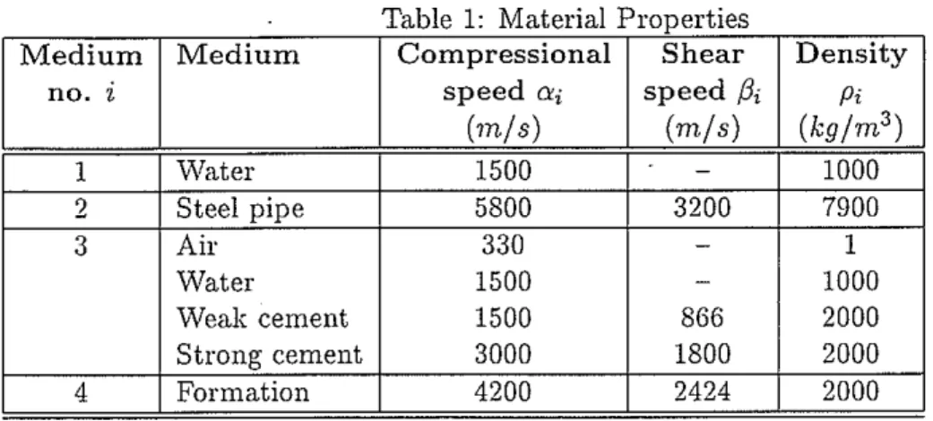
Table 1- Material Properties

Medium Medium Compressional Shear Density

no. i speed "'i speed f3i _Pi

(mls) (mls) (kglm3) 1 Water 1500 - 1000 2 Steel pipe 5800 3200 7900 3 Air 330 - 1 Water 1500 - ₁₀₀₀ Weak cement 1500 866 2000 Strong cement 3000 1800 2000 4 Formation 4200 2424 2000 (

(9)

Transmitter

Near receiver

Far receiver

Annulus

(10)

Air channel -3r---~---, - 3 r - - - ,Water channel -4 ... -4 .. _-5 . OJ :!1. c o ~-6 , .

"

c j!J <f.-7 .. -5 . -6 .. -8 .. -8 ... -9:----~---'---' 0 2 4 6 6 4 - 9 ' - - - ' - - - - ' - - - ' o 2

Weak cement channel (P Impedance

=

3.0)

- 8 r - - - - ' , - - - , _-8r---~---,Strong cement channel (P impedance=6

-9 -9 .. -10 -10 . ~-11 c ~-12

"

c .!! ;;:-13 -11 .. -12 0 . n v _ 13 '0::"0 . .==ir.c=~"""""'cc<>=~ -14 .. -15 .. _-15 -16'---~---'----'

o

2 4 6

Channel thickness [inch]

o

-16:----~--__c_---J

0 2 4 6

\.

Figure 2: Casing thickness variation: c,

=

0.25 in; Annulus thickness H

=

0.3; 0.6, 0.9, 2, 3, 4, 5 and 6 in; Annulus = air; water, weak cement and strong cement; Transducer separations t,.rTR=t,.r12

=

6 in; Stand-off distance X

=

0.5 in; Ricker source wavelet center freq. = 80-200 kHz, in steps of 20 kHz, with 80 kHz result shown in gray (multiply attenuations in the plot by 2 for attenuation in units of dB/ft).

(11)

6 6 Air channel

-3,---.,---,---,

-4 ... ~-5 .

'"

:>!.

"

~ -6 , .

"

~ «-7 . -8 -9~---'---'-_ _..J o 2 4

Weak cement channel (P impedance=3.0) -6,--:---,---~---, -7 . -8~' -12 . -13 -14~--~---'-_ _--.J o 2 4

Channel thickness [inch]

Water channel

- 3 , - - - _ - - _ - - . . . ,

-4 -5 . -6 . -7 . -8 -9~---:':----'-

_ _

..J

o

2 4 6

Strong cement channel (P impedance=6

-6,---_---:._----:.-..., -7 -8 . -9 . -10 .9...~.. v o -11 o -12"" . -13 -14~---::----'--_--.J

o

2 4 6

=

0.3,-0.6,

0.9, 2, 3, 4, 5 and 6 in; Annulus = air, water, weak cement and strong cement; Transducer separations Ll.rTR=Ll."12

=

0.5 in; Ricker source wavelet center freq. = 80-200 kHz, in steps of 20 kHz, with 80 kHz result shown in gray (multiply attenuations in the plot by 2 for attenuation in units of

(12)

Air channel Water channel - 4 , - - - , - 4 , - - - , -5 . -5 . -6 -6

co

-7 :!2. c o ~ -8

"

§ :;c -9 -8 . -9 .... -10 -10 -11 -11 6 -12'---'---'~--...Jo 2 4 6 -12 ' - - - ' - - - - " - - - ' 0 2 4 (

Weak cement channel (P Impedance

=

3.0)

- 6 , - - - , - 6 , - - - . , . - - - ,Strong cement channel (P impedance

=

6

-7 . -7 . _8"""· _-8 iIi' -9 . :!2. c o ~-10 , ~..

"

c 2 :;c-11

.:::::==:==:=::=::::=~

~2"""""""'" ~3··· -12~."~ . ICl~

-13~

~=::=~=::=~==*

-14~--~---'---...J

o

2 4 6

-14 ' -_ _-'-_ _---'-_ _--.J

0 2 4 6

=

0.3, 0.6, 0.9, 2, 3, 4, 5 and 6 in; Annulus = air, water, weak cement and strong cement; Transducer separations D.rTR=D.r12

=

(13)

in 0". c o .~ ::l C Q) ;j'

Source-receiver spacing = 3 [inch]

-4

-5

-6

Source-receiver spacing = 6 [inch]

-9

- 10L---'---'----'---'----'-_-'--'---'---'-.J

10-1 10°

_ 15L---'---'----'----'---'-_-'--'----'---'-.J

10-1 10°

Channel thickness [Inch]

Figure 5: Transducer separation variation: fl1"TR=fl1"12 = 3 and 6 in; Annulus thickness H = 0.1-6 in; Annulus = strong cement, Casing thickness = 0.35 in; Stancl-off distance X

=

0.5 in; Ricker source wavelet center freq.

=

80-200 kHz, in steps of 20 kHz, with 80 kHz result shown in gray (multiply attenuations in the left plot by 4 and the right plot by 2 for attenuation in units of clB/ft).

(14)

Air channel Water channel

..

+ + o + + -15 -10 . -5 + """"'-';";;~' .

..

"

-5 . o + OJ ~-10 <= o ~_:> <= .$-15 .

«

-20 -20 . -25'--'---'--~~~-'----l o 2 4 6 8 10 10 8 6 4 2 -25 '----''----'---'---'---'----' o (

Weak cement channel (P Impedance=3.0)

O,-~-~-~-:...--, Strong cement channel (P impedance

_{0 . - - - ,}

=6

-5 OJ ~-10 . <= .Q "iii :> <= .$-15

«

+ 0 -5 "0' ., .... , -10 . + -15 ... -20 -20 ..:1:" . ( -25,.-~--':"_-:---'--,.,....---.J o 2 4 6 8 10

Transducer separation [inch]

-25'--~_--'-_-'-_~_~---.J

o

2 4 6 8 10

Figure 6: 'Transducer separation variation: f1"TR=f1r12 = 1-12 in; Annulus thickness H = 0.5 in; Annulus = air, water, weak cement and strong cement; Casing thickness

=

0.35 in; Stand-off distance X

=

0.5 in; Ricker source wavelet center freq.

=

80 kHz (gray lines with '0') and 200 kHz (black lines with '+').

(15)

Air channel Water channel _25~~---"---':---,;---:':,---.J

o

2 4 6 8 10 + + + + o + + _5. 0 -20 . -15 -10 .. 0 -5 iii' 31.-10 c: 0

₊

~

"

c: 2-15· :;: + 0 -20 -25 0 2 4 6 6 10

Weak cement channel (P Impedance=3.0)

Or-~---, Strong cement channel (P impedanceOr-~---,=6

-10 .... -20 . + o -5 + -15 . -5 ··0·· iii' !!.-10 c:

~

"

c: ~-15 ..: + 0 -20 _25l-_~_~---,~---',----'::--J o 2 4 6 8 10

-25L---"_---':_---:-_--:-_:':---'

o

2 4 6 8 10

Figure 7: Transducer separation variation: ll.rTR=ll.r12 = 1-12 in; Annulus thickness

H

=

1 in; Annulus

=

air, water, weak cement and strong cement; Casing thickness = 0.35 in; Stand-off distance X = 0.5 in; Ricker source wavelet center freq. = 80 kHz (gray lines with '0') and 200 kHz (black lines with '+').

(16)

Travel times of various wavetypes 6 , - - - , - - - , - . , . - - - , - - , - - - r - - - " , - - - - , 120 100 80 . ... - _ . Comp: refri3.cted· . Shearrefr~cted Direct ..~~!I~.qt~.q.:

pomp. and shearrefractedwave~ 11IylqQmR~1r~faqtga

60

Time [micro sec]

40 • 0 ~" o·

..

.

..

...

..

,,-. o

.

• o o o o ... o o o o

.

:/ ·0 o ...

.

..

:. .

.

• o

.

o

.

o o ... o

.

20

a

c .2

iii

'"

:B-3

w :;;

"

::> 1:J w c i"2 f-5 134_c =

(17)

Air channel Water channel -3r---~--~---' -3r---~--~~--, -4 -4 -5 -6 ...-... -7 -6 -9 6 0 2 4 6 4 2 _9l.--_~_ _~ ~_ _..J

o

-8 .. ~ a 15-6 " . => ~ g -<-7 ..

Weak cement channel (P Impedance = 3.0) -6r--~---~----'

Strong cement channel (P impedance=6

-6r---~---~----' -7 .. _-7 " -8 .~. _-8 W -9 !!. -9 .. ~ a 'iii-10 .;; . =>

~

g::t:=::=::=::=::=:1

2 n ;;:-11 . -11 o o -12 .. -12 'n .. -13 -13 ...,,:: ... n . .. 6 _14L-_ _~ ~_ _....J o 2 4

6 _14L-_ _~ ~_ _....J

o 2 4

Figure 9: Stand-off distance variation: X

=

0.3, 0.6, 0.9, 2, 3, 4, 5 and 6 in; Annulus = air, water, weak cement and strong cement; Transducer separations 6.TTR=D.'·12

=

6 in; Casing thickness Ct

=

(18)

Air channel Water channel -3r---~---, - 3 r - - - , -4 . -4 .... _-5 co :!2.

"

a ~-6

""

jg "" -7 . -5 -6 -7 -6 -6 6 4 2 _9 ' - - - - ' - - - ' - - - - ' o 6 4 2 - 9 ' - - - - ' - - - - ' - - - ' o

Weak cement channel (P Impedance=3.0) - 6 r - - - ,

Strong cement channel (P impedance=6 - 6 r - - - , -7 -7 ( -6 :~ . _-6

co

-9 :!2. § ~-10

""

2 ;;:-11 -9 ( -12 -12 . ....; . 6 -13

·u~··~

"..

~.

':==::==::==::==::==*

-14 ' - - - ' - - - ' - - - ' o 6 2 4

-14 ' - - - ' - - . - - - - ' - - - '

o

-13

Figure 10: Stand-off distance variation: X

=

1 in; Annulus thickness H

=

0.3, 0.6,

0.9 , 2, 3, 4, 5 and 6 in; Annulus = air, water, weak cen1ent and strong cen1entj

Transducer separations LlTTR=Ll"12 = 6 in; Casing thickness c, = 0.35 in; Ricker source wavelet center freq. = 80-200 kHz, in steps of 20 kHz, with 80 kHz result shown in gray (multiply attenuations in the plot by 2 for attenuation in units of