HAL Id: hal-01544879
https://hal.inria.fr/hal-01544879v2
Submitted on 30 May 2017
HAL is a multi-disciplinary open access
archive for the deposit and dissemination of
sci-entific research documents, whether they are
pub-lished or not. The documents may come from
teaching and research institutions in France or
abroad, or from public or private research centers.
L’archive ouverte pluridisciplinaire HAL, est
destinée au dépôt et à la diffusion de documents
scientifiques de niveau recherche, publiés ou non,
émanant des établissements d’enseignement et de
recherche français ou étrangers, des laboratoires
publics ou privés.
Less effective selection leads to larger genomes
Tristan Lefébure, Claire Morvan, Florian Malard, Clémentine François, Lara
Konecny-Dupré, Laurent Guéguen, Michèle Weiss-Gayet, Andaine
Seguin-Orlando, Luca Ermini, Clio Der Sarkissian, et al.
To cite this version:
Tristan Lefébure, Claire Morvan, Florian Malard, Clémentine François, Lara Konecny-Dupré, et al..
Less effective selection leads to larger genomes. Genome Research, Cold Spring Harbor Laboratory
Press, 2017, 27, pp.1016-1028. �10.1101/gr.212589.116�. �hal-01544879v2�
Less effective selection leads to larger genomes
Tristan Lef´
ebure
1, Claire Morvan
1, Florian Malard
1, Cl´
ementine Fran¸cois
1, Lara
Konecny-Dupr´
e
1, Laurent Gu´
eguen
4, Mich`
ele Weiss-Gayet
2, Andaine
Seguin-Orlando
3, Luca Ermini
3, Clio Der Sarkissian
3, N. Pierre Charrier
1, David
Eme
1, Florian Mermillod-Blondin
1, Laurent Duret
4, Cristina Vieira
4,5, Ludovic
5
Orlando
3,6, and Christophe Jean Douady
1,51
Univ Lyon, Universit´e Claude Bernard Lyon 1, CNRS UMR 5023, ENTPE, Laboratoire d’Ecologie des Hydrosyst`emes Naturels et Anthropis´es, F-69622 Villeurbanne, France
2
Univ Lyon, Universit´e Claude Bernard Lyon 1, CNRS UMR 5310, INSERM, Institut NeuroMyoG`ene, F-69622 Villeurbanne, France
10
3
Center for GeoGenetics, Natural History Museum of Denmark, University of Copenhagen, Øster Voldgade 5-7, 1350K Copenhagen, Denmark
4Univ Lyon, Universit´e Claude Bernard Lyon 1, CNRS UMR 5558, Laboratoire de Biom´etrie et Biologie Evolutive, F-69622 Villeurbanne, France
5Institut Universitaire de France, F-75005 Paris, France
15
6
Universit´e de Toulouse, University Paul Sabatier (UPS), CNRS UMR 5288, Laboratoire AMIS, F-31073 Toulouse, France
March 23, 2017
Corresponding author: [email protected] Running title: Less effective selection leads to larger genomes
20
Keywords: Genome size, effective population size, transposable elements, selection efficacy, Asel-lidae, groundwater
Abstract
The evolutionary origin of the striking genome size variations found in eukaryotes remains enig-matic. The effective size of populations, by controlling selection efficacy, is expected to be a key
25
parameter underlying genome size evolution. However, this hypothesis has proved difficult to investigate using empirical datasets. Here, we tested this hypothesis using twenty-two de novo transcriptomes and low-coverage genomes of asellid isopods, which represent eleven independent habitat shifts from surface water to resource-poor groundwater. We show that these habitat shifts are associated with higher transcriptome-wide dN/dS. After ruling out the role of positive selection
30
and pseudogenization, we show that these transcriptome-wide dN/dSincreases are the consequence
of a reduction in selection efficacy imposed by the smaller effective population size of subterranean species. This reduction is paralleled by an important increase in genome size (25% increase on average), an increase also confirmed in subterranean decapods and mollusks. We also control for an adaptive impact of genome size on life history traits but find no correlation between body size, or
35
growth rate, and genome size. We show instead that the independent increases in genome size mea-sured in subterranean isopods are the direct consequence of increasing invasion rates by repeated elements, which are less efficiently purged out by purifying selection. Contrary to selection efficacy, polymorphism is not correlated to genome size. We propose that recent demographic fluctuations and the difficulty to observe polymorphism variations in polymorphism-poor species can obfuscate
40
the link between effective population size and genome size when polymorphism data is used alone.
Introduction
Eukaryotic organisms exhibit striking variations in their genome size (GS). Within animals, the range of GS extends from 20 Mb in the roundworm Pratylenchus coffeae to 130 Gb in the lungfish Protopterus aethiopicus (Gregory, 2005a). GS shows no correlation with organism complexity, an
45
observation early referred to as the C-value paradox (Thomas, 1971). Even though the contribution of mechanisms such as polyploidization events or transposable element amplification to DNA gain or loss is now better understood (Gregory, 2005b), the evolutionary origin of GS variation still remains largely unexplained (Petrov, 2001).
Large genomes mostly consist of non-coding DNA (Gregory, 2005b; Lynch, 2007). The origins
50
of the large variations in the amount of non-coding DNA found across eukaryotes are currently ten-tatively explained through two opposite sets of theories. Adaptive theories postulate that variation of the amount of non-coding DNA results in significant phenotypic changes and thus evolves under
the control of natural selection. Main examples of phenotypic changes commonly associated to GS variations include nucleus and cellular sizes (Cavalier-Smith, 1982), growth rate (Grime and
Mow-55
forth, 1982) and metabolic rate (Vinogradov, 1995) variations. Conversely, non-adaptive theories postulate that GS variations have little phenotypic impact (Doolittle and Sapienza, 1980), leaving non-adaptive forces such as mutation and genetic drift as the main evolutionary drivers underlying GS variation (Lynch and Conery, 2003). In particular, the mutational-hazard (MH) hypothesis sug-gests that slightly deleterious mutations, including those that lead to GS variation, can segregate
60
in small populations where the efficacy of purifying selection is impaired by genetic drift (Lynch et al., 2011; Lynch, 2011). Under this hypothesis, the evolution of GS would be controlled by the balance between the emergence of large-scale insertions and deletions (indels) and their fixation rate, which ultimately depends on the efficacy of selection and, thus, the effective population size (Ne).
65
Phylogenetic inertia, varying mutational patterns and uncertainties in Ne estimates, are but a
few difficulties that complicate testing of the MH hypothesis with empirical evidence. While GS appears to correlate negatively with population size in eukaryotes (Lynch and Conery, 2003), in agreement with the MH hypothesis, this relationship vanishes when accounting for phylogenetic non-independence among taxa (Whitney and Garland, 2010). In addition, predictions of the MH
70
hypothesis can vary in opposite directions depending on the underlying pattern of indel mutations. In eukaryotes, where indel mutation patterns are typically biased toward insertions, reductions in population size are predicted to lead to increasing GS. Conversely, similar Ne reductions are
expected to result in decreasing GS in bacteria, for which the mutation pattern is biased toward deletions (Kuo et al., 2009). Moreover, although essential to the MH hypothesis, Ne remains
75
difficult to estimate. Most studies rely on population polymorphism (Lynch and Conery, 2003) or heterozygosity (Yi and Streelman, 2005), two measures that typically reflect population size history over the last tens of thousands to millions of generations, while the pace of genome evolution might take place at much longer temporal scales (Whitney and Garland, 2010; Whitney et al., 2011).
Since the formulation of the MH hypothesis, the few early empirical studies that originally
80
supported a relationship between GS and Ne (Lynch and Conery, 2003; Yi and Streelman, 2005)
have been criticized (Whitney and Garland, 2010; Gregory and Witt, 2008) and later analyses failed to support this relationship. No relationships were found between GS and (i) allozyme polymorphism in plants (Whitney et al., 2010), (ii) molecular polymorphism among different species of rice (genus Oryza, Ai et al., 2012), and (iii) the relative population size in seed beetles (Arnqvist
85
Finally, the influence of Neon Caenorhabditis has been dismissed in favor of an adaptive explanation
(Fierst et al., 2015). However, all these studies suffered either from the use of very indirect proxies of Ne or from small gene samples, often characterized for not more than 12 species (although
exceptions exist, see Whitney et al., 2010). Therefore, the influence of Ne on GS remains to be
90
tested on an empirical dataset that provides a robust estimate of Newithin a statistically powerful
framework.
Habitat shifts often result in drastic changes in population size and therefore offer useful case studies for testing the MH hypothesis. In this study, we use a comparative genomic approach to test whether non-adaptive forces drive changes in GS following the habitat shift from surface water
95
to groundwater within asellid isopods. The colonization of groundwater from surface water took place at multiple times and locations over the last tens to hundreds million years ago within this family (Morvan et al., 2013), thereby providing independent replicates of the transition to dark and low-energy habitats (Venarsky et al., 2014; Huntsman et al., 2011). Groundwater colonization leads to eye-degeneration and is considered irreversible (Niemiller et al., 2013). We use 11 pairs of
100
closely-related surface and subterranean asellid species to test the predictions of the MH hypothesis (Table S1). According to the MH hypothesis and assuming that consistent population size reduction took place following groundwater colonization, then, subterranean species are predicted to show reduced selection efficacy and larger GS than their surface relatives. We also considered alternative hypotheses, namely (i) the possible reduction in GS in response to energy limitation in groundwater,
105
and (ii) the selection of particular life history traits (hereafter, growth rate and body size) as a driver of patterns of GS variation.
Results
Efficacy of natural selection in groundwater
To evaluate differences in selection efficacy between surface and subterranean species, we sequenced
110
and de novo assembled the transcriptomes of 11 pairs of asellid species. After gene families de-limitation, we estimated the rate of non-synonymous over synonymous substitutions (dN/dS) on a
set of conserved and single copy genes. This ratio is jointly defined by the distribution of selection coefficient of new mutations (s) and the magnitude of genetic drift as defined by Ne (Nielsen and
Yang, 2003). Therefore, the transcriptome-wide dN/dSis expected to increase over extended
peri-115
ods of small Nebecause of the increasing fixation of slightly deleterious mutations (Ohta, 1992), an
transcriptome-wide dN/dS is a direct proxy of selection efficacy. Subterranean species show significantly higher
transcriptome-wide dN/dSthan their surface relatives (Figure 1, Table 1). Looking at each pair of
species independently, 8 pairs out of 11 display a higher subterranean transcriptome-wide dN/dS,
120
a relative increase that can be as high as 59% (Figure 1).
While long periods of reduced Ne will induce higher transcriptome-wide dN/dS, adaptation to
new habitats could potentially produce the same effect. Under the action of positive selection, ben-eficial non-synonymous mutations will reach fixation faster than their synonymous counterparts and will lead to sites with dN/dS> 1. If the frequency of such sites increases during the transition
125
to groundwater, then, we can expect the transcriptome-wide dN/dSto increase. We first tested this
adaptive hypothesis using a model that allows dN/dSvariation across sites and makes it possible to
differentiate between variation in the intensity of purifying (w−) and positive selection (w+) and their respective frequencies. Subterranean species do not show an elevated frequency (f q(w+)) or
intensity of positive selection (w+) but show higher w− (Table 1 & S2, Figure S1 & S3). This
sup-130
ports a scenario in which subterranean species do not experience higher rates of positive selection, but instead evolve under reduced purifying selection efficacy.
We next tested the adaptive dN/dS increase scenario using polymorphism data. Under high
rate of positive selection with recurrent fixation of non-synonymous mutations, populations will display an excess of non-synonymous substitutions compared to non-synonymous polymorphism
135
(McDonald and Kreitman, 1991). We used the “direction of selection” statistics (DoS, Stoletzki and Eyre-Walker, 2011), which is a transcriptome-wide comparison of the rates of non-synonymous substitution and polymorphism, to test if positive selection indeed led to higher rates of fixation in subterranean species (DoS > 0). Most subterranean species have negative DoS (Figure S4) and subterranean species do not have higher DoS than surface species (Table 1). On the contrary, in
140
most species, irrespective of their habitat, the DoS is close to 0 or negative indicating that many slightly deleterious mutations are segregating in these species. While this observation is in line with the idea that effective population sizes reduces the efficacy of selection in these species, it does not completely rule out the hypothesis that subterranean species may have concomitantly evolved higher dN/dSas a result of more frequent adaptations during the shift from surface to subterranean
145
habitats. When slightly deleterious mutations dominate the evolutionary dynamics, which appears to be the case in this group, they can mask the influence of adaptive evolution on polymorphism (James et al., 2016). We further tested this hypothesis by directly estimating the rate of adaptation (α) in two species pairs where subterranean species display elevated dN/dSthan their surface sister
species (P. beticus versus P. jalionacus and P. coiffaiti versus P. cavaticus, Figure 1). We used
a McDonald-Kreitman (McDonald and Kreitman, 1991) modified approach (Messer and Petrov, 2013) designed to cancel the influence of demography and linkage effects. For species such as the ones studied here, the high prevalence of segregating deleterious mutations at low frequency inflates the rate non-synonymous polymorphism and artificially decrease α estimates. Messer and Petrov suggest to reconstruct α as a function of the derived allele frequencies. As allele frequency increases,
155
slightly deleterious alleles become rarer, to the point that a robust estimate of α can be obtained by calculating the asymptotic α for an allele frequency of 1. By re-sequencing the transcriptomes of 4 to 5 individuals per species, we reconstructed the unfolded site frequencies of these two pairs of species, fitted the distribution of α(x) and estimated the asymptotic α(1). For each species we recovered the expected distribution of α(x) as in Messer and Petrov (2013) and obtained asymptotic
160
α that were negative (Figure S5). While subterranean species of these two pairs of species show clear transcriptome-wide dN/dSincreases, they do not display elevated rate of adaptation. For one
pair there is no significant α variation (P. beticus - P. jalionacus, p-value=0.49), while in the other pair the subterranean species shows lower α estimates (P. coiffaiti - P. cavaticus, p-value=0.02). Therefore both DoS and α analyses confirm that the increase in dN/dS in subterranean species
165
is not caused by a higher rate of positive selection, in line with the results found on the model differentiating between variation in the intensity of purifying (w−) and positive selection (w+).
Subterranean species share multiple convergent regressive phenotypes, such as the loss of eyes and pigmentation which may ultimately be associated with gene non-functionalizations (Protas et al., 2005; Niemiller et al., 2013). A transcriptome-wide dN/dS increase can therefore also be
170
caused by an excess of genes that have lost their function and consequently have acquired dN/dS
nearing 1. As an example, the opsin gene of subterranean species has much higher dN/dSas a result
of gene non-functionalization (see next section and Figure S6). Release of functional constraint on a gene and the resulting dN/dSincrease should also be paralleled with much lower gene expression,
if no expression at all (Zou et al., 2009; Yang et al., 2011). This is typically observed for the
175
opsin gene that has much lower expression in the subterranean species (Figure S6). If gene non-functionalization in subterranean species is pervasive enough to shift the transcriptome-wide dN/dS
upwards, we expect to see a subset of genes with lower expression in the subterranean species. We tested this hypothesis by comparing the expression of the genes in the surface and subterranean species of each pair. The set of conserved and single copy genes that was used to calculate each
180
species dN/dS have much higher expression levels than the complete transcriptomes (Figure S7).
This set of genes also displays more conserved gene expression levels across species (Figure S7). Finally, after counting changes in gene expression category between sister species, we found no
evidence of an excess of genes with lower expression in the subterranean species (Wilcoxon signed rank test p-value=0.650, Table S4). We further tested this non-functionalization hypothesis by
185
looking for a subset of genes that would display larger dN/dSin the subterranean species while the
remaining genes would display no dN/dS variation. Distributions of the variation in gene dN/dS
did not support the existence of such a small subset of genes (Figure S2). On the contrary, these distributions were unimodal with a median positively correlated to the transcriptome-wide dN/dS
(R2 = 0.62, p-value = 0.004).
190
Altogether, we accumulated multiple evidences that the transcriptome-wide dN/dS increase
observed in subterranean species is not the consequence of increased levels of positive selection or gene non-functionalization, but rather the result of convergent reductions in the efficacy of purifying selection among subterranean species.
Polymorphism proxies of N
e195
Instead of directly assessing selection efficacy, the MH hypothesis has traditionally been tested using polymorphism data. Indeed, polymorphisms provide a direct proxy for Ne, which tunes the
magnitude of genetic drift and ultimately the efficacy of selection. As transcriptomes were sequenced from pooled individuals, we estimated synonymous and non-synonymous polymorphism for genes with high coverage. We used the population mutation rate (ˆθw) which is proportional to the product
200
of Neand the mutation rate µ, and the ratio of non-synonymous over synonymous polymorphism
(pN/pS), which is expected to decrease with increasing Ne, independently of µ. Both the dN/dS
and the pN/pS measure the efficacy of selection to purge slightly deleterious mutations, though
the later works at a much shorter timescale. As expected, ˆθwand pN/pSare negatively correlated
(phylogenetic generalized least-squares models, PGLS p-value <0.001, R2= 0.43). Polymorphism
205
data are generally consistent with selection patterns inferred from dN/dS: subterranean species
have significantly higher pN/pS than their surface relatives in 6 out of 11 pairs, whereas there is
no pair significantly supporting the opposite pattern (Figure 1). However for ˆθw the pattern is less
clear: in 6 pairs subterranean species have significantly lower ˆθw, while in 3 pairs subterranean
species show significantly higher ˆθw (Figure 1). Overall, the differences in pN/pS or ˆθw between
210
subterranean and surface species are not statistically significant (Table 1). In addition, there is no correlation between ˆθwor pN/pSand the efficacy of selection as estimated using the
transcriptome-wide dN/dS (PGLS p-value=0.80 and 0.79, respectively). Traditional polymorphism proxies of Ne
Estimating colonization times with opsin sequences
215
Subterranean species may have colonized groundwater at different time periods, some being sub-terranean for a much longer time than others. Ignoring such differences through the use of a qualitative present-day ecological status (i.e. surface versus subterranean) may limit our power to detect a change in GS or polymorphism associated with the subterranean transition. One could contrast polymorphism measures and the time since the latest speciation event, where we know
220
that a species ancestor was a surface species, but this would only be valid if speciation and col-onization times were synchronous. Alternatively, we estimated the colcol-onization time using the non-functionalization of the opsin gene. Indeed, similarly to observations made in underground mammals (Emerling and Springer, 2014), together with the regression of the ocular system, some subterranean species display loss-of-function mutations in eye pigment (Leys et al., 2005) or opsin
225
genes (Niemiller et al., 2013), which are indicative of a loss of functional constraint. If we assume that opsin gene sequences have lost their function early in the process of groundwater colonization, then, they must have been evolving under a neutral model (dN/dS = 1) since that colonization.
Using a two states model of evolution with one surface opsin dN/dS estimated using opsins from
surface species, and one subterranean opsin dN/dSequal to 1, we can then estimate the colonization
230
time as a function of the speciation time and the estimated opsin dN/dSmeasured on a given branch
leading to a subterranean species.
Using a combination of Sanger sequencing, transcriptome assemblies and genome sequencing reads, we reconstructed one opsin ortholog for 19 species out of 22. Irrespective of their ecological status, the two species of the genus Bragasellus probably do not possess this opsin locus. In
addi-235
tion, for one Proasellus subterranean species (P. parvulus), failure to amplify or recover Illumina reads from this locus suggests that the whole locus was lost in this species. Subterranean species showed lower opsin expression levels and had much higher opsin dN/dS ratios than surface species
(average dN/dS = 0.3 and 0.05, respectively, Figure S6). In addition to one subterranean species
which completely lost the loci (P. parvulus), two subterranean species also harbored clear
non-240
functionalization signatures consisting of an 18 base-long deletion for P. solanasi and the insertion of a 280 base-long repeated element in the sequence of P. cavaticus. These observations validate the opsin locus as a colonization clock.
Estimated colonization times vary a lot with more than 50X variation between the youngest subterranean species (P. jalionacus, 2 MYA) and the oldest one (P. herzegovinensis, 122 MYA,
245
Table S5). Colonization time is related to the regression of the eye and pigmentation, with species with intermediate phenotypes (reduced eyes and partial depigmentation) being very recent
sub-terranean species (Figure S8). Using relative colonization time (timecolonization
timespeciation ) for dN/dS ratios or
absolute colonization time instead of the present-day ecological status gives very similar results (Ta-ble 1), indicating that variations in the colonization time are not likely to obfuscate polymorphism
250
variations. Conversely, the strength of the correlation between the transcriptome-wide dN/dS (or
w−) and relative colonization time is higher than with the ecological status (Table 1), reinforcing the hypothesis of a causal link between the subterranean colonization and the subsequent drop in selection efficacy. The only exception is the frequency of sites under positive selection (f q(w+),
Table 1) which becomes significantly higher in subterranean species when colonization time is used
255
instead of ecological status (PGLS p-value=0.016, +0.6% per 100 MY of colonization).
Genome size increase in groundwater
We next measured genome sizes in all 11 species pairs using flow cytometry. Using either the ecological status or the colonization time, we found a statistically significant increase in GS following the transition from surface to groundwater habitats (Figure 1, Table 1). Looking at each pair of
260
species independently, 7 pairs out of 11 display a significantly higher GS, a relative increase reaching 137% in P. hercegovinensis (Figure 1). This finding is robust to the addition of 19 asellid species (PGLS with 41 asellids, p-value= 0.022, coefficient=0.273) and to the inclusion of a wider range of metazoans (linear mixed model with 18 independent pairs including Decapoda and Gastropoda, p-value = 0.040, 25% average increase in GS, Figure 2, Table S6).
265
Linking genome size to selection efficacy
One of the main predictions of the MH hypothesis is that GS is negatively correlated with selection efficacy in eukaryotes. We validated this prediction because we found a highly significant positive relationship between GS and the transcriptome-wide dN/dS(or w−, Table 1, Figure S9). In addition
the dN/dSratio (or w−) achieves similar, if not better, performance in predicting GS variation than
270
the ecological status or colonization time (lower AIC and higher R2, Table 1). When d
N/dS(or w−)
is put first and ecological status second into a single PGLS model of GS, the effect of the ecological status is no longer significant (PGLS p-value=0.189).
Testing other covariates
In contradiction to the MH hypothesis, adaptative hypotheses postulate that variation in GS is
275
parameters (such as body size and growth rate) (Gregory, 2001). In many species, population size covaries with traits under selection such as growth rate and body size, themselves correlated to some extent to GS, making any causation test extremely challenging (Gregory, 2005b). While body size was readily available in the literature, we estimated growth rate in 16 species using the RNA/protein
280
ratio which is known to be positively correlated to growth rate in Rotifera (Wojewodzic et al., 2011). Indeed, in situ estimates of growth rates were out of reach, and a more traditional proxy such as the RNA/DNA ratio is inapplicable when GS varies. In accordance to the general assumption that subterranean animals tend to adopt K-selection life history traits, subterranean asellids species display lower growth rate, though no trend was found regarding body size (Table 1). However,
285
growth rate and body size do not correlate with GS (Table 1, Figure S9). Thus, although many forces might be at play during the transition to groundwater habitats, in asellids, we only found correlation between selection efficacy and GS.
Mechanism of genome size increase
Implicit in the MH hypothesis is that an increase in GS should result from the progressive spread
290
of insertions with slightly deleterious fitness effects, such as transposable elements (Vieira et al., 2002). Yet, other much faster mechanisms such as polyploidization events can also inflate GS (Otto, 2007). We tested for the occurrence of such large duplication events by looking for an excess of recent paralogs in the 11 subterranean species compared to their surface sister species. The mean number of gene copy per gene family is not correlated to the ecological status nor to GS (PGLS
295
p-value=0.773 and 0.579, respectively, Figure S10), indicating that subterranean species do not present an excess of recent duplication events.
To test for the accumulation of repeated elements, we evaluated the amount of repeated DNA in the 11 asellid species pairs using low-coverage genome sequencing, followed by clustering of the highly repeated elements. Indeed, contrary to the non-repeated fraction of the genome, elements at
300
high frequency will collect enough reads to be assembled. Summing across the contributions of each element provides an estimate for the size of the repeatome (ie. the fraction of the genome consisting of repeated DNA elements). We found larger repeatomes in large genomes (Figure 3A & D, Table 2, Figure S11). The repeatomes are largely made of repeat families found in a single species, called repeat orphans, with very few shared repeats across species (Figure 3B). The occurrence of these
305
shared repeats is largely explained by phylogenetic relatedness: closely related sister species share more than 200 repeat families with this number quickly decreasing with divergence time (Figure 3C). GS has little power to explain the composition of the repeatome. None of the axes of a repeatome
composition correspondence analysis is correlated to GS while the first three axes harbor a strong phylogenetic signal (Blomberg K > 1 with p-value < 0.01, Table S7, Figure S12).
310
The pattern of GS increase is globally congruent with a global increase of the repeatome inva-siveness. Indeed, big genomes have at the same time more repeats and repeats at higher frequencies (Table 2, Figure 3E & D). To a lesser extent, the number of repeat orphans and their frequencies also increase with GS (Table 2), demonstrating that big genomes are also more prone to genome invasion by new repeats. Nonetheless, the ratio of the total genomic size (TGS) occupied by new
315
repeats over common repeats do not change ( TGSorphans
TGSnon−orphans, Table 2), indicating that this aspect
of the repeat community structure does not change as GS increases. So, contrary to several model organisms such as humans or maize, the GS increase was not induced by a very limited set of ele-ments, but is the consequence of a repeat element community that became globally more invasive subsequently to the ecological transition.
320
While the repeated portion of the genome increases linearly with GS, it does not explain 100% of GS variations: on average 1Gb of repeats was gained for 1.3Gb of GS increase (Table 2). Con-sequently, the estimated TGS of the non-repeated portion of the genome also increases with GS, though at a much slower pace (1Gb for 2.8Gb, Table 2). Either repeats are harder to assemble in large genomes or another minor mechanism is also at play during GS increase. Directly using
325
the repeatome size instead of GS in correlation analyses gives similar or reinforced results: while polymorphism based Ne proxies (ˆθw or pN/pS), growth rate and body size do not correlate with
repeatome size, selection efficacy (dN/dSor w−) does (Table 1).
Discussion
We found a substantial correlation between selection efficacy, as measured by transcriptome-wide
330
dN/dS, and repeatome size. This finding indicates that, for a large part, GS is controlled by the
efficacy of selection to prevent the invasion of the genome by repeated elements. Conversely, we found no correlation between Neestimates derived from polymorphism data and GS. At first glance,
this result sounds contradictory since the efficacy of selection depends on Ne. We propose two
non-mutually exclusive hypotheses to explain this contradiction. First, while the transcriptome-wide
335
dN/dS provides an average estimate of selection efficacy since the divergence of two species of a
pair, polymorphism-based proxies such as ˆθw or pN/pS are influenced by recent Ne fluctuations,
independently of the divergence time. If Ne fluctuates rapidly with large amplitude around a
This hypothesis is supported by larger coefficients of variations for ˆθwor pN/pSthan for the dN/dS
340
(CVdN/dS = 0.22, CVpN/pS= 0.39, CVθˆw= 0.73, test of the equality of CVs p-value < 0.001). In this
study, we observed the effect of multiple groundwater transitions that happened tens to hundreds million years ago, a time scale long enough to produce large dN/dS and GS variations, but also
encompassing important climatic fluctuations which potentially generated shorter time-scale Ne
variations. Particularly, quaternary climatic fluctuations are likely to have produced important Ne
345
fluctuations in surface species which have much more unstable habitats than subterranean species. Therefore, the lack of a clear correlation between short-term Ne proxies, like polymorphism, and
GS might be the consequence of recent climatic fluctuations. Interestingly, this hypothesis received some support using Tajima’s D tests. Indeed, only P. beticus (a surface species) out of the 4 species for which we have adequate data to estimate Tajima’s D is not at the mutation-drift equilibrium
350
(p-value=0.017, Table S8). This surface species shows evidence of recent population contraction (Tajima’s D > 0) which might explain its unexpected combination of low polymorphism and low dN/dSwhen compared to its sister subterranean species (Figure 1). Second, polymorphism variation
might also be more prone to measurement artifacts than dN/dS. In particular, SNP calling errors
can constitute a relatively important fraction of detected variants among species with low levels of
355
polymorphism. For most species pairs (7 out of 11), we observed a higher level of polymorphism in surface than in subterranean species (Figure 1, Figure S13). The four other cases all correspond to pairs for which both species have low level of polymorphism, which might therefore be subject to higher measurement error rates. This is in line with the strong relationship observed between the surface species ˆθw and the difference in ˆθw between species pairs (R2 = 0.74, p-value < 0.001,
360
Figure S13). This suggests that below approximately 2, ˆθw becomes a poor indicator of Ne
changes. Altogether, the use of polymorphism proxies of Ne for polymorphism-poor species or for
species which experienced recent Nevariations might therefore result in misleading rejection of the
MH hypothesis.
Our findings shed new light on the debate of the validity of the MH hypothesis and the
com-365
parative methods that should be implemented to test it (Charlesworth and Barton, 2004; Gregory and Witt, 2008; Whitney and Garland, 2010; Lynch, 2011; Whitney et al., 2011). Using a relatively reduced set of ecologically-contrasted species pairs as true replicates of the same ecological transi-tion is statistically more powerful than testing for differences in genomic attributes among a larger set of distantly related taxa, in which the number of independent observations is unknown and for
370
which many traits varies. Accounting for phylogenetic effects in statistical analyses of GS variation among multiple species is another yet crucial aspect because it increases not only specificity
(Whit-ney and Garland, 2010) but also sensitivity. Taken altogether, subterranean species do not have larger GS than surface species (ordinary least square linear model p-value = 0.122 for the 11 species pairs, p-value = 0.095 for the 41 asellid species, p-value = 0.261 for the 18 metazoan species pairs),
375
whereas pairwise comparisons of surface and subterranean species (Figure 1 & 2) and PGLS models (Table 1) reveal a very clear and significant pattern of higher GS among subterranean species.
While there is several lines of evidence supporting a lower selection efficacy caused by long-term Ne reduction in subterranean species, we found little support that the colonization of this new
habitat was also paralleled with adaptive evolution. The only evidence was found in the frequency
380
of sites under positive selection when colonization time was used. The increase was nonetheless moderate (+0.6% per 100 MY of colonization) and was not supported by polymorphism (DoS or α) analyses. However, this study is limited to a small set of gene families that are found in most species, in a single copy and whose expression is very conserved. This set of genes is probably under strong purifying selection and might be less prone to positive selection. Fully investigating
385
the relative role of adaptive versus non-adaptive forces during this ecological transition will require a much broader genomic approach.
Disentangling the forces that drive GS variation has commonly been complicated by rampant covariation between GS and multiple traits such as cell and body sizes, growth rates, metabolism and Ne, to name a few. In this study, we found no association between GS and two common covariates
390
(body size and growth rate). While we cannot completely rule out other non-tested parameters and alternative ad hoc adaptive hypotheses, the results of this study are fully compatible and best explained by a causal relationship between Ne and GS. The mechanisms that drive genome size
variation are also fully compatible with the MH hypotheses. The repeated elements were globally more diversified and more invasive in species with reduced selection efficacy, an expected outcome
395
if selection against repeated element proliferation is less effective.
Documenting changes in the architecture of genomes among taxa that have undergone major shifts in habitats (Protas et al., 2005; Jones et al., 2012; Fang et al., 2014; Soria-Carrasco et al., 2014) holds much promise for disentangling evolutionary processes driving genome evolution. According with the MH hypothesis, our focus on the genomics of groundwater colonization brings new evidence
400
for a prominent role of non-adaptive forces in GS evolution. Despite strong energetic constraints in groundwater, GS likely increases under the long-term effect of reduced Ne, which limits the
strength of natural selection in hampering the invasion of slightly deleterious repeated elements. Altogether this study supports long-term effective population size variation as a key evolutionary regulator of genome features.
Methods
Aselloidea timetree
Phylogenetic comparative methods require accurate estimates of phylogenetic relationships and divergence times among species (Purvis et al., 1994). Both were inferred from a large timetree of Aselloidea containing 193 evolutionary units (Morvan et al., 2013) (Table S9). Sequences of the
410
mitochondrial cytochrome oxidase subunit I (COI) gene, the 16S mitochondrial rDNA gene and the 28S nuclear rDNA gene used to build the Aselloidea timetree were obtained according to methods described in (Calvignac et al., 2011; Morvan et al., 2013). Alignments and Bayesian estimates of divergence times were conducted according to (Morvan et al., 2013). From the Aselloidea timetree, we selected 11 independent pairs of surface and subterranean asellid species as replicates of the
415
ecological transition from surface water to groundwater.
RNA-seq
For the 11 selected species pairs (Table S1) individuals were sampled from caves, springs, wells, and the hyporheic zone of streams using different pumping and filtering devices (Bou-Rouch pump, Cvetkov net, and Surber sampler) and were flash frozen alive. Total RNA was isolated using
420
TRI Reagent (Molecular Research Center, Cincinnati, USA). Extraction quality was checked on a Bioanalyser RNA chip (Agilent Technologies, Santa Clara, USA) and RNA concentrations were estimated using a Qubit fluorometer (Thermo Fisher Scientific, Waltham, USA). Prior to any addi-tional analysis, species identification was corroborated for each individual by sequencing a fragment of 16S gene. Equimolar pools of at least 5 individuals were made to achieve 10µg of the total RNA
425
(Table S1). Volumes were reduced using a Concentrator-Plus (Eppendorf, Hamburg, Germany) to achieve approximately 10µL. Double strand poly(A)-enriched cDNA were then produced using the Mint2 kit (Evrogen, Moscow, Russia) following the manufacturer protocol except for the first-strand cDNA synthesis, where the CDS-1 adapter was used with the plugOligo-Adapter of the Mint1 kit (5’ AAGCAGTGGTATCAACGCAGAGTACGGGGG P 3’). After sonication with a Bioruptor Nextgen UCD300
(Diagen-430
ode, Lige, Belgium) and purification with MinElute (Qiagen, Hilden, Germany), Illumina libraries were prepared using the NEBNext kit (New England BioLabs, Ipswich, USA) and amplified using 22 unique indexed primers. After purification with MinElute, 400-500 base pair fragments were size selected on an agarose gel. Libraries were paired-end sequenced on a HiSeq 2000 sequencer (Illu-mina, San Diego, USA) using 100 cycles at the Danish National High-throughput DNA Sequencing
435
reads were resampled to represent about 2%, 5%, 10%, 25%, 50% and 100% of a full lane. These 6 sets of reads were de novo assembled (see next section) and the number of assembled components > 1kb was compared among sets (Figure S14). This preliminary experiment was used as a rational procedure to multiplex 4 species on one lane.
440
Transcriptome assembly
Adapters were clipped from the sequence, low quality read ends were trimmed (phred score <30) and low quality reads were discarded (mean phred score <25 or if remaining length <19bp) using fastq-mcf of the ea-utils package (Aronesty, 2013). Transcriptomes were de novo assembled using Trinity (version 2013-02-25, Grabherr et al., 2011). Open reading frames (ORF) were identified
445
with TransDecoder (http://transdecoder.sourceforge.net/). For each assembled component, only the longest ORF was retained, and gene families were delimited using all against all BLASTP (Altschul et al., 1990) and SiLiX (Miele et al., 2011). SiLiX parameters were set to i=0.6 and r=0.6 as they were maximizing the number of 1-to-1 orthologous gene families.
d
N/d
Scalculation
450
Single copy orthologs were extracted for 3 different sets of taxa: the 11 asellid species pairs (320 genes), the ibero-aquitanian clade (863 genes), and the alpine-coxalis clade (2257 genes) (see Fig-ure 1). Each gene family was then aligned with the following procedFig-ure: (1) search and masking of frameshift using MACSE with frameshift cost set to -10 (Ranwez et al., 2011), (2) multiple align-ments of the translated sequences with PRANK (L¨oytynoja and Goldman, 2008) using the empirical
455
codon model and F option, (3) site masking with Gblocks (Castresana, 2000) using -t=c, -b5=h and -b2 set as -b1. After gene concatenation, a transcriptome-wide dN/dSratio was estimated with
the free ratio model of CODEML from the package PAML 4.7a (Yang, 2007). Confidence intervals were obtained using 100 non-parametric bootstrap samples (random sampling of the codon sites with replacement).
460
To test whether the observed dN/dS increase could be attributed to a reduction in the efficacy
of purifying selection or to an increase in positive selection (a higher number of sites under positive selection and/or an elevated positive selection intensity), we used the M10 branch-site model (Yang et al., 2000) as implemented in BppML (Dutheil and Boussau, 2008). To reduce computation times, the analysis was performed using quartets of taxa: the two species of a pair and two additional
465
surface species used to root the tree. Large alignments (>300 000 codons) were reduced by randomly sampling 280 000 codons and only sites that were complete were retained. Purifying and positive
selection intensity (w− and w+) and frequency (f q(w−) and 1 − f q(w−)) were estimated using the a posteriori mean site dN/dSusing BppMixedLikelihoods (Dutheil and Boussau, 2008).
Single nucleotide polymorphism
470
Estimating population polymorphism from pooled RNA-seq samples is complicated by the fact that (1) RNA-seq is prone to both RT-PCR and sequencing errors (Gout et al., 2013), (2) polymorphism can be over-estimated by hidden paralogs (Gayral et al., 2013), and (3) it is difficult to differentiate low frequency alleles from sequencing errors in pooled data-sets (Futschik and Schl¨otterer, 2010). While an accurate estimate is currently out of reach, it is possible to obtain polymorphism estimates
475
that are comparable across taxa. We developed a statistical design that (1) is conservative in defining polymorphism, (2) balances the sampling effort so that estimates obtained within a species pair are comparable and (3) maximizes the number of analyzed genes to gain statistical power. Single nucleotide polymorphism (SNP) was searched on a set of 5027 gene families that were present as a single copy in at least 6 out of the 11 species pairs. Gene famillies with hidden paralogs were
480
filtered by using 10X coverage DNA-seq data available for 4 species (P. karamani, P. hercegovinenis, P. ibericus and P. arthrodilus). Gene families that had a DNA-seq coverage higher than the 90th percentile in any of these 4 species were filtered for any further polymorphim analysis. RNA-seq reads were aligned on the assembled ORF using BWA (aln algorithm, (Li and Durbin, 2009)). SAMtools (Li et al., 2009) was then used to generate a BAM file, discard duplicated reads, and
485
export a BCF file. SNPs were filtered and called with bcftools and vcfutils.pl with the following conservative filtering parameters: minimum read depth of 10, minimum number of reads supporting an allele of 4, and minimum distance to a gap set to 15. Then, SNPs were classified as synonymous or non-synonymous. Only the genes that were highly covered in both species of a pair (average coverage >50X, same results were obtained with lower coverage cutoff) were further considered to
490
compute transcriptome-wide summary statistics (Table S3). This design ensured that synonymous and non-synonymous polymorphism estimates could be compared across taxa, although each of these estimates might be over or under estimated. We then calculated the population mutation rate (θ) using the Watterson estimator:
ˆ θw= pS P2n−1 i=1 1 i
with pS the frequency of synonymous segregating sites and n the number of pooled individuals.
495
Con-fidence intervals were obtained by bootstrapping the genes 10000 times.
This polymorphism data-set was also used to measure the direction of selection statistics (DoS, Stoletzki and Eyre-Walker, 2011) using:
DoS = Dn
Dn+ Ds
− Pn
Pn+ Ps
with Ds and Dn the number of synonymous and non-synonymous divergences, and Ps and Pn
500
the number of synonymous and non-synonymous polymorphisms. Divergences where measured with PAML 4.7a (Yang, 2007) and polymorphisms using the above described pipeline. DoS were measured gene by gene for every species pairs and compared for every pair using a wilcoxon signed rank test or globally using the median DoS per species.
Rate of adaptation and Tajima’s D
505
For two species pairs (P. beticus, P. jalionacus, P. coiffaiti and P. cavaticus), we performed addi-tional RNA-seq 50 base single-end Illumina sequencing, but this time by independently sequencing 4 to 5 individuals per species owing the estimation of allele frequencies. Reads were mapped on the assembled transcriptomes using BWA (mem algorithm, (Li and Durbin, 2009)), and SNPs were called using Reads2snp (Gayral et al., 2013). The site frequency spectrum (SFS) were than unfolded
510
using the alignment with the respective sister species orthologs. Only sites with non-ambiguously reconstructed ancestral and derived allele were kept. We then used Messer and Petrov approach (Messer and Petrov, 2013) to directly estimate the proportion of adaptive substitutions (α) from the unfolded-SFS. Confidence intervals for α were obtained by bootstrapping the SNP 1000 times. The same dataset was also used to test if population were at the mutation-drift equilibrium using
515
Tajima’D test (Tajima, 1989).
Colonization time
For 19 species, we were able to determine the sequence of one opsin gene. Sequences were determined using (i) transcriptome sequences, (ii) Sanger sequencing using (Taylor et al., 2005) PCR primers (LWF1a and Scylla) and PCR conditions, and (iii) genomic Illumina reads as detailed bellow. For
520
the latter, reads were mapped on the closest available opsin sequence following the same approach as for the SNP search and a consensus was called with the Samtools program suite.
To estimate colonization time, we used the loss of function observed in several subterranean species and postulated that the opsin gene loss-of-function took place at the time of groundwater
colonization. We used a model with two dN/dS ratios, one for the functional opsins (ωsurf) and
525
one for the non-functional opsin (ω1) which was set to 1. We then defined the dN/dSof a branch
leading to a subterranean taxa (ωsubt) as the weighted mean between these two defined ratios, such
as: ωsubt = ωsurf T − t T + ω1 t T
with T the speciation time, and t the time of colonization. From this, we estimated the time of colonization as follows:
530
t = T ×ωsubt− ωsurf 1 − ωsurf
Another relevant parameter is the proportion of time a species has been subterranean since the divergence with its sister species, named the relative colonization time (RCT ), which we estimated using:
RCT = t T =
ωsubt− ωsurf
1 − ωsurf
Opsin dN/dSwere estimated using PAML free-ratio branch model, and the ωsurf was estimated as
the average dN/dSof the surface species showing the most obvious surface phenotypes (P. coiffaiti,
535
P. coxalis, P. karamani, P. ibericus, P. meridianus and P. beticus).
Measurement of genome size
We measured GS for 41 species of asellid (including the 11 species pairs), 4 Atyidae (Pancrustacea, Decapoda) and 2 Rissoidae (Mollusca, Gastropoda) (Table S6). After sampling, individuals were preserved at ambient temperature in silica gel. Measurements were conducted according to (Vieira
540
et al., 2002). Nuclei were extracted from the head of organisms (or from entire individuals when body size was less than 3 mm in length). Heads were crushed in 200µL of cold modified Galbraiths nuclei isolation buffer (20 mM MOPS, 20.5 mM MgCl2, 35.5 mM trisodium citrate, 0.1% Triton X-100, 20µg mL−1 boiled RNase A, pH 7.2 adjusted with NaOH; (Galbraith et al., 1983)). The mixture was filtered through 100µm and then 30 µm mesh-size nets. The filtrate was centrifuged
545
during 10 sec at 2600g and the supernatant was carefully removed. Pellets were resuspended in 200µL of nuclei isolation buffer. The resuspension was again centrifuged during 10 sec at 2600g and the supernatant was carefully removed. Pellets were resuspended in 250µL of buffer and transferred in 5 mL polystyrene round-bottom tubes. An amount of 50µL of propidium iodure was added to each tube. Tubes were kept in ice and darkness until GS measurements.
550
Instru-ments) fitted with an argon laser at 488-nm wavelength. We analyzed 5 individuals per species. Individuals were measured in a random order and two individuals of the same species were never analyzed in the same run. Samples were calibrated to two external standards: Drosophila virilis females (GS of 0.41 pg, Bosco et al., 2007) and Asellus aquaticus (GS of 2.49 pg, Rocchi et al.,
555
1988, and authors’ cross validation). The Drosophila were maintained under laboratory conditions at 25 ◦C for two to three generations before GS measurements. Standards were prepared using the protocol described above from 5 organism heads and were measured in each run (2 measures for D. virilis at the beginning and end of runs and 5 measures for A. aquaticus evenly distributed during the runs).
560
The FlowQ bioconductor package (Gentleman et al., 2004) in R software (R Core Team, 2013) was used for quality assessment of flow cytometry data. All the flow cytometer analyses were checked for cell number, boundary events and time anomalies. Cell subsetting known as gating, was firstly performed manually using the BD FACSDiva software (BD Biosciences). Secondly, the automatic curvHDR filtering method (Naumann et al., 2010) was used to select the cells located
565
in the highest density region (HDR level = 0.8). Then, when drift over time was significant, gated values were corrected using a linear regression on A. aquaticus reference using the following equation: IPcoor= IPx−IPIPx
st× (x − x0) × λ, where IPcorr is the corrected gated value, IPxis the
gated value to correct, IPst is the A. aquaticus reference gated value at the beginning of the run
(time t = x0) estimated by the linear regression, x is the measurement time for the gated value
570
to correct, x0 is the time at the beginning of the run and λ is the slope of the linear regression
on A. aquaticus reference. Drift was considered significant when the regression on A. aquaticus reference had adjusted R2 values ≥ 0.1. Finally, GS were derived from fluorescence data using
D. virilis as a standard for Asellidae and Rissoidae and using A. aquaticus as a standard for Atyidae. Indeed, large GS in Atyidae (previously known GS range from 3.30 to 7.20 pg, Gregory,
575
2005a) prevented the use of D. virilis as a standard.
Growth rate and body size
Growth rates were estimated using the total RNA normalized by the total protein biomass of an organism (RNA/protein ratio, Wojewodzic et al., 2011) for at least 7 individuals per species. Total RNA and proteins were isolated using TRI Reagent (Molecular Research Center). RNA
580
concentrations were calculated by fluorometry with a Qubit (Life Technologies). Total proteins were obtained using the Bicinchoninic acid assay (Smith et al., 1985). Body size were estimated using maximum body size as reported in each species description.
Genome sequencing
To compare the size of the repeatome between surface and subterranean species, we sequenced the
585
genome of the 11 pairs of Asellidae species. For 4 species (P. ibericus, P. arthrodilus, P. karamani, P. hercegovinensis), we built blunt-ended libraries for shotgun sequencing on Illumina platforms, as described in (Orlando et al., 2013; Seguin-Orlando et al., 2013) with few modifications. Oneµg of DNA in 100µL TE buffer was sheared using a Bioruptor NGS device (Diagenode) with four cycles of 15 seconds ON/90 seconds OFF. The obtained size distributions of sheared DNA fragments were
590
centered at around 500 bp. After concentration in 22µL EB buffer (Qiagen) with the MinElute PCR Purification kit (QIAGEN), the sheared DNA fragments were built into blunt-ended DNA libraries using the NEBNext Quick DNA Library Prep Master Mix Set for 454 (New England BioLabs, reference nb. E6070L), following the protocol described in (Meyer and Kircher, 2010), but with 0.5µM Illumina adapters (final concentration). All reactions were carried out in 25 µL
595
volumes; incubation times and temperatures were as follows: 20 min at 12◦C, 15 min at 37◦C for end-repair; 20 min at 20◦C for ligation; 20 min at 37◦C, 20 min at 80◦C for fill-in. After the end-repair and ligation steps, reaction mixes were purified using the MinElute PCR Purification Kit (Qiagen) using elution volumes of 16µL and 22 µL of EB buffer, respectively. The final 25 µL volume of blunt-end libraries was split in two parts and PCR amplified independently in 50µL
600
reaction mixes containing: 5 units Taq Gold (Life Technologies), 1X Gold Buffer, 4 mM MgCl2, 1 mg/ml BSA, 0.25 mM of each dNTP, 0.5µM of Primer inPE1.0 (5’-AAT GAT ACG GCG ACC ACC GAG ATC TAC ACT CTT TCC CTA CAC GAC GCT CTT CCG ATC T-3) and 0.5µM of an Illumina 6 bp-indexed (I) primer (5-CAA GCA GAA GAC GGC ATA CGA GAT III III GTG ACT GGA GTT CAG ACG TGT GCT CTT CCG-3). Thermocycling conditions for
the amplifications were: activation at 92◦C for 10 min; followed by nine cycles of denaturation at
605
92◦C for 30 sec, annealing at 60◦C for 30 sec, elongation at 72◦C for 30 sec; and final elongation at 72◦C for 7 min. PCR products were purified using the MinElute PCR Purification kit, with a final elution volume of 25µL EB buffer.
For the remaining 18 species, we built Illumina TruSeq DNA PCR-free LT libraries (Illumina, catalog FC-121-3001), following manufacturers recommendations. Briefly, 1µg of DNA extract
610
was sheared in a total volume of 50µL TE buffer, using a Bioruptor NGS device (Diagenode) with three cycles of 25 seconds ON/90 seconds OFF. The fragmented DNA was cleaned up using Illumina Sample Purification Beads. After end-repair, the DNA fragments were size-selected around 350bp using two consecutive bead purification steps, A-tailed, and ligated to 6bp-indexed Illumina TruSeq adaptors (Set A). Two last bead purifications were performed to remove any adaptor dimer and
615
for contaminations, library and PCR blanks were carried out at the same time as the samples. Amplified libraries and blanks were quantified using the 2100 Bioanalyzer (Agilent) High-Sensitivity DNA Assay. No detectable amount of DNA could be recovered from the blanks. Blunt-End indexed DNA libraries were pooled and sequenced on two lanes of a HiSeq 2000 Illumina platform (100 cycles
620
paired-end mode run), while the two PCR-free libraries pools were sequenced each on one flow-cell of the Hiseq 2500 Illumina platform (150 paired-end run, Rapid Mode, 6bp index read), at the Danish National High-Throughput DNA Sequencing Centre.
Repeatome size estimates
We used low coverage read sequencing to characterize repeated genome sequences (Nov´ak et al.,
625
2010) using RepeatExplorer (Nov´ak et al., 2013). Prior to analysis, DNA-seq reads were randomly sampled to achieve 0.05X coverage following the GS estimated by flow cytometry, so that estimates are comparable across taxa. After clustering of the reads into highly repeated elements by Re-peatExplorer, the number of reads representing each repeated element is a direct function of the repeat frequency, the GS, and the sequencing effort. The proportion of the genome (GP) made
630
by this repeat is GPi = nreadsi/nreads, with nreadsi the number of reads making the repeat i,
and nreads the total number of reads. The proportion of genome made of repeats (the repeatome
size) is then GP =P
iGPi. By default, RepeatExplorer filters repeat elements that have genome
proportion lower than 0.01%. To achieve comparable estimates independent of genome sizes, the number of repeats or the repeatome size of a given genome were recalculated by filtering repeats
635
that occupied less than 0.5 Mb. A repeat element total genomic size (TGS) was then calculated as T GSi = GPi× GSj with GSj the genome size of species j. Repeat families were delimited using
blastn (e-value=0.1) and SiLiX (i=50 and r=70).
Comparative analyses
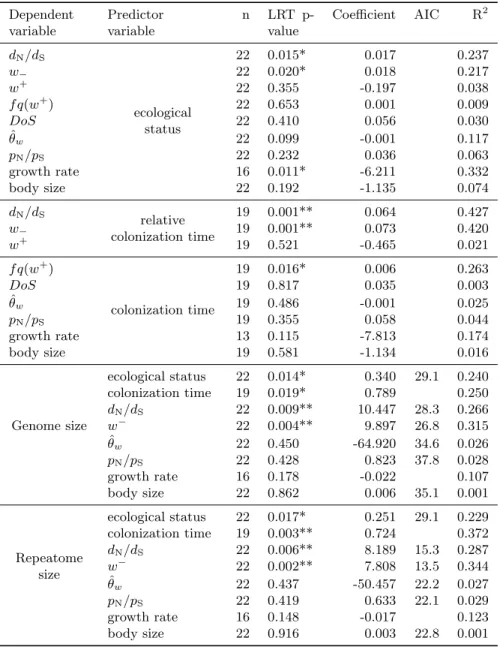
Phylogenetic generalized least squares (PGLS) regression models (Martins and Hansen, 1997) were
640
used to test for the correlation between 2 variables. We first tested the association between the ecological transition and population size, biological traits or GS (top of Table 1). PGLS were also used to test for the association between GS and population size, biological traits (bottom of Table 1) or genomic features (Table 2). The correlation between two variables was assessed by comparing a model without the predictor variable (intercept model) to a model including the predictor variable
645
using a likelihood ratio test (LRT). Analyses were performed in R using ape (Paradis et al., 2004) and nlme (Pinheiro et al., 2014) packages. The best model of trait evolution and its associated
covariance structure, in our case the Brownian motion model, was selected according to minimum Akaike information criterion (AIC). The difference in ˆθw, pN/pS, and dN/dSbetween the two species
of a surface - subterranean pair was tested using the proportion of bootstrap replicates supporting
650
a difference (critical level = 5%) and the difference in GS was tested using a Wilcoxon rank sum test with 5 measurements of GS (ie. 5 individuals) per species. We also performed ordinary least squares models to test for the effect of the ecological status on GS while ignoring phylogenetic relationships among species. To test for the effect of the ecological transition on GS using a wider range of taxa (ie. 18 species pairs including Decapoda and Mollusca with 5 measurements of GS per
655
species), we performed a linear mixed model in R using the nlme package because a chronogram with accurate branch length could not be obtained given the available molecular markers and calibration points. The ecological status (ie. surface versus subterranean) was a fixed effect, and we specified the random error structure as ecological status nested into species pairs to account for phylogenetic relationships among species. Then, we performed the model with no hierarchy in the
660
random error structure, which is equivalent to an ordinary least squares model, to test for the effect of the ecological status on GS while ignoring phylogenetic relationships among species. Differences in the coefficient of variations of different variables were tested using modified signed-likelihood ratio test (Krishnamoorthy and Lee, 2014) using the R package cvequality.
Data access
665
Sequence reads and assemblies have been deposited to the European Nucleotide Archive (ENA;
http://www.ebi.ac.uk/ena) under the study accession numberPRJEB14193. Sanger sequences were
submitted to NCBI (GenBank; https://www.ncbi.nlm.nih.gov/nucleotide/) under the accession numbers KC610091-KC610505 (Table S9).
Acknowledgments
670
This work was supported by the Agence Nationale de la Recherche (ANR-08-JCJC-0120-01 DEEP, ANR-15-CE32-0005 Convergenomix); the Institut Universitaire de France; the European Commis-sion (7th EU Framework Programme, Contract No. 226874, BioFresh), the CNRS (APEGE No. 70632, PEPS ExoMod 2014 and Enviromics 2014), the french embassy in Denmark, the Danish National Research Foundation (DNRF94) and the Marie-Curie Intra-European Fellowship (IEF
675
biolog-ical material: Alhama de Granada municipality, Besson JP, Bodon M, Bouillon M, Capderrey C, Carreira I, Chatelier B, Colson-Proch C, Creuz´e des Chatelliers M, Cueva de Valporquero, Culver D, Datry T, Delegacion provincial de medio ambiente Ronda, Ferrandini J, Ferrandini M, Fiser C, Fong D, Gina D, Gottstein S, Gouffre de Padirac, Kaufmann B, Knight L, Lana E, Le Pennec R,
680
Lescher-Moutoue F, Magniez G, Messana G, Michel G, Nassar E, Nassar-Simon N, Notenboom J, Orozco R, Parc National du Mercantour, Parco Naturale Alta Valle Pesio e Tanaro, Planes S, Pri´e V, Reboleira AS, Sauve municipality, Sendra A, Simon L, Sket B, Stoch F, Turjak M and Zag-majster M. We thank the laboratory technicians at the Danish High-throughput DNA Sequencing Centre for technical assistance. We thank Boulesteix M, Burley N, Goubert C, Paradis E and Simon
685
L for providing advices on the analyses, Bi´emont C and Schaack S for their advices or comments on earlier drafts of this manuscript. We gratefully acknowledge support from the CNRS/IN2P3 Com-puting Center (Lyon/Villeurbanne - France), for providing a significant amount of the comCom-puting resources needed for this work. This work was performed using the computing facilities of the CC LBBE/PRABI. We thank 2 anonymous reviewers and Adam Eyre-Walker for their comments.
690
Disclosure declaration
The authors declare no conflicts of interest.
References
Ai B, Wang ZS, and Ge S. 2012. Genome size is not correlated with effective population size in the oryza species. Evolution 66: 3302–3310.
Altschul SF, Gish W, Miller W, Myers EW, and Lipman DJ. 1990. Basic local alignment search tool. J. Mol. Biol. 215: 403–410.
Arnqvist G, Sayadi A, Immonen E, Hotzy C, Rankin D, Tuda M, Hjelmen CE, and Johnston JS. 2015. Genome size correlates with reproductive fitness in seed beetles. Proc. R. Soc. Lond., B, Biol. Sci. 282: 20151421. Aronesty E. 2013. Comparison of sequencing utility
pro-grams. Open Bioinformatics Journal 7: 1–8. Bosco G, Campbell P, Leiva-Neto JT, and Markow TA.
2007. Analysis of drosophila species genome size and satellite dna content reveals significant differences among strains as well as between species. Genetics 177: 1277–1290.
Calvignac S, Konecny L, Malard F, and Douady CJ. 2011. Preventing the pollution of mitochondrial datasets with nuclear mitochondrial paralogs (numts). Mitochondrion 11: 246–254.
Castresana J. 2000. Selection of conserved blocks from multiple alignments for their use in phylogenetic anal-ysis. Mol. Biol. Evol. 17: 540–552.
Cavalier-Smith T. 1982. Skeletal dna and the evolution of genome size. Annu. Rev. Biophys. Bioeng. 11: 273– 302.
Charlesworth B and Barton N. 2004. Genome size: does bigger mean worse? Curr. Biol. 14: R233–R235. Doolittle WF and Sapienza C. 1980. Selfish genes, the
phenotype paradigm and genome evolution. Nature 284: 601–603.
Dutheil J and Boussau B. 2008. Non-homogeneous mod-els of sequence evolution in the bio++ suite of libraries and programs. BMC Evol. Biol. 8: 255.
Emerling CA and Springer MS. 2014. Eyes underground: regression of visual protein networks in subterranean mammals. Mol. Phylogenet. Evol. 78: 260–270. Fang X, Nevo E, Han L, Levanon EY, Zhao J, Avivi
A, Larkin D, Jiang X, Feranchuk S, Zhu Y, et al.. 2014. Genome-wide adaptive complexes to under-ground stresses in blind mole rats spalax. Nat. Com-mun. 5: 10.1038/ncomms4966.
Fierst JL, Willis JH, Thomas CG, Wang W, Reynolds RM, Ahearne TE, Cutter AD, and Phillips PC. 2015. Reproductive mode and the evolution of genome size and structure in caenorhabditis nematodes. PLoS Genet. 11: e1005323.
Futschik A and Schl¨otterer C. 2010. The next generation of molecular markers from massively parallel sequenc-ing of pooled dna samples. Genetics 186: 207–218. Galbraith DW, Harkins KR, Maddox JM, Ayres NM,
Sharma DP, and Firoozabady E. 1983. Rapid flow cytometric analysis of the cell cycle in intact plant tis-sues. Science 220: 1049–1051.
Galtier N. 2016. Adaptive protein evolution in animals and the effective population size hypothesis. PLoS Genet. 12: 1–23.
Gayral P, Melo-Ferreira J, Gl´emin S, Bierne N, Carneiro M, Nabholz B, Lourenco JM, Alves PC, Ballenghien M, Faivre N, et al.. 2013. Reference-free population ge-nomics from next-generation transcriptome data and the vertebrate–invertebrate gap. PLoS Genet. 9: e1003457.
Gentleman RC, Carey VJ, Bates DM, Bolstad B, Det-tling M, Dudoit S, Ellis B, Gautier L, Ge Y, Gentry J, et al.. 2004. Bioconductor: open software devel-opment for computational biology and bioinformatics. Genome Biol. 5: R80.
Gout JF, Thomas WK, Smith Z, Okamoto K, and Lynch M. 2013. Large-scale detection of in vivo transcription errors. Proc. Natl. Acad. Sci. U.S.A. 110: 18584– 18589.
Grabherr MG, Haas BJ, Yassour M, Levin JZ, Thomp-son DA, Amit I, Adiconis X, Fan L, Raychowdhury R, Zeng Q, et al.. 2011. Full-length transcriptome assem-bly from RNA-Seq data without a reference genome. Nat. Biotechnol. 29: 644–652.
Gregory TR. 2001. Coincidence, coevolution, or causa-tion? dna content, cellsize, and the c-value enigma. Biological Reviews 76: 65–101.
Gregory TR. 2005a. Animal genome size database. http://www.genomesize.com.
Gregory TR. 2005b. The evolution of the genome. Else-vier, San Diego.
Gregory TR and Witt JD. 2008. Population size and genome size in fishes: a closer look. Genome 51: 309– 313.
Grime J and Mowforth M. 1982. Variation in genome size – an ecological interpretation. Nature 299: 151–153. Huntsman BM, Venarsky MP, Benstead JP, and Huryn
AD. 2011. Effects of organic matter availability on the life history and production of a top vertebrate predator (plethodontidae: Gyrinophilus palleucus) in two cave streams. Freshwat. Biol. 56: 1746–1760.
James JE, Piganeau G, and Eyre-Walker A. 2016. The rate of adaptive evolution in animal mitochondria. Mol. Ecol. 25: 67–78.
Jones FC, Grabherr MG, Chan YF, Russell P, Mauceli E, Johnson J, Swofford R, Pirun M, Zody MC, White S, et al.. 2012. The genomic basis of adaptive evolution in threespine sticklebacks. Nature 484: 55–61. Krishnamoorthy K and Lee M. 2014. Improved tests for
the equality of normal coefficients of variation. Com-putational Statistics 29: 215–232.
Kuo CH, Moran NA, and Ochman H. 2009. The conse-quences of genetic drift for bacterial genome complex-ity. Genome Res. 19: 1450–1454.
Leys R, Cooper SJ, Strecker U, and Wilkens H. 2005. Regressive evolution of an eye pigment gene in inde-pendently evolved eyeless subterranean diving beetles. Biol. Lett. 1: 496–499.
Li H and Durbin R. 2009. Fast and accurate short read alignment with burrows–wheeler transform. Bioinfor-matics 25: 1754–1760.
Li H, Handsaker B, Wysoker A, Fennell T, Ruan J, Homer N, Marth G, Abecasis G, Durbin R, et al.. 2009. The sequence alignment/map format and sam-tools. Bioinformatics 25: 2078–2079.
L¨oytynoja A and Goldman N. 2008. Phylogeny-aware gap placement prevents errors in sequence alignment and evolutionary analysis. Science 320: 1632–1635. Lynch M. 2007. The origins of genome architecture,
vol-ume 98. Sinauer, Sunderland.
Lynch M. 2011. Statistical inference on the mechanisms of genome evolution. PLoS Genet. 7: e1001389. Lynch M, Bobay LM, Catania F, Gout JF, and Rho M.
2011. The repatterning of eukaryotic genomes by ran-dom genetic drift. Annu. Rev. Genomics Hum. Genet. 12: 347–366.
Lynch M and Conery JS. 2003. The origins of genome complexity. Science 302: 1401–1404.
Martins EP and Hansen TF. 1997. Phylogenies and the comparative method: a general approach to incorpo-rating phylogenetic information into the analysis of in-terspecific data. Am. Nat. pp. 646–667.
McDonald JH and Kreitman M. 1991. Adaptive protein evolution at the Adh locus in Drosophila. Nature 351: 652–654.
Messer PW and Petrov DA. 2013. Frequent adaptation and the mcdonald-kreitman test. Proc. Natl. Acad. Sci. U.S.A. 110: 8615–8620.
Meyer M and Kircher M. 2010. Illumina sequencing li-brary preparation for highly multiplexed target cap-ture and sequencing. Cold Spring Harbor Protocols 2010: pdb.prot5448.
Miele V, Penel S, and Duret L. 2011. Ultra-fast sequence clustering from similarity networks with SiLiX. BMC Bioinformatics 12: 116.
Mohlhenrich ER and Mueller RL. 2016. Genetic drift and mutational hazard in the evolution of salamander genomic gigantism. Evolution 70: 2865–2878. Morvan C, Malard F, Paradis E, Lef´ebure T,
Konecny-Dupr´e L, and Douady C. 2013. Timetree of aselloidea reveals species diversification dynamics in groundwa-ter. Syst. Biol. 62: 512–522.
Naumann U, Luta G, and Wand MP. 2010. The curvhdr method for gating flow cytometry samples. BMC Bioinformatics 11: 44.