Nonnegative control of finite-dimensional linear systems

(1)

HAL Id: hal-02335968

https://hal.archives-ouvertes.fr/hal-02335968

Submitted on 28 Oct 2019

HAL is a multi-disciplinary open access

archive for the deposit and dissemination of

sci-entific research documents, whether they are

pub-lished or not. The documents may come from

L’archive ouverte pluridisciplinaire HAL, est

destinée au dépôt et à la diffusion de documents

scientifiques de niveau recherche, publiés ou non,

émanant des établissements d’enseignement et de

Nonnegative control of finite-dimensional linear systems

Jérôme Lohéac, Emmanuel Trélat, Enrique Zuazua

To cite this version:

Jérôme Lohéac, Emmanuel Trélat, Enrique Zuazua. Nonnegative control of finite-dimensional linear

systems. Annales de l’Institut Henri Poincaré (C) Non Linear Analysis, Elsevier, 2021, 38 (2),

pp.301-346. �10.1016/j.anihpc.2020.07.004�. �hal-02335968�

(2)

Nonnegative control of finite-dimensional linear systems

Jérôme Lohéac

∗

_{Emmanuel Trélat}

†

_{Enrique Zuazua}

‡§¶

Abstract

We consider the controllability problem for finite-dimensional linear autonomous control systems with nonnegative controls. Despite the Kalman condition, the unilateral nonnegativity control constraint may cause a positive minimal controllability time. When this happens, we prove that, if the matrix of the system has a real eigenvalue, then there is a minimal time control in the space of Radon measures, which consists of a finite sum of Dirac impulses. When all eigenvalues are real, this control is unique and the number of impulses is less than half the dimension of the space. We also focus on the control system corresponding to a finite-difference spatial discretization of the one-dimensional heat equation with Dirichlet boundary controls, and we provide numerical simulations.

Keywords: Minimal time, Nonnegative control, Dirac impulse.

Résumé

Dans cet article, nous considérons la contrôlabilité d’un système linéaire avec des contrôles positifs. Malgré la condition du rang de Kalman, la condition de positivité des contrôles peut conduire à l’existence d’un temps minimal de contrôlabilité strictement positif. Lorsque tel est le cas, nous démontrons que si la matrice du système de contrôle possède une valeur propre réelle, alors il existe dans l’espace des mesures de Radon positives, un contrôle en le temps minimal et ce contrôle est nécessairement une somme finie de masse de Dirac. De plus, lorsque toutes les valeurs propres de la matrice sont réelles, ce contrôle est unique et le nombre de masses de Dirac le constituant est d’au plus la moitié de la dimension de l’espace d’état. Nous particularisons ces résultats sur l’exemple de l’équation de la chaleur unidimensionnelle, avec des contrôles frontières de type Dirichlet, discrétisée en espace et nous proposons quelques simulations numériques.

Mots clefs :Temps minimal, Contrôles positifs, Impulsions de Dirac.

1 Introduction and main results

Let n∈ IN∗, A be an n× n real-valued matrix and B be an n × 1 real-valued matrix, such that the

pair(A, B) satisfies the Kalman condition. We consider the finite-dimensional linear autonomous control system

˙

y(t) = Ay(t) + Bu(t) (1.1) where controls u are real-valued locally integrable functions. Given any initial state y0_{∈ IR}n _and

any final state y1_{∈ IR}n_{, the Kalman condition implies that the control system (1.1) can be steered}

from y0 _{to y}1 _{in any positive time. In other words, the minimal controllability time required to}

pass from y0 _{to y}1 _{is zero.}

Now, we impose the unilateral nonnegativity control constraint

u(t) ⩾ 0 (t > 0 a.e.). (1.2) It has been shown in [20] that such a constraint may induce a positive minimal controllability time (this is also the case for unilateral state constraints). Actually, for every y0_{∈ IR}n_{, there exists a}

target y1_{∈ IR}n _{such that the minimal time required to pass from y}0 _{to y}1_{is positive.}

The objective of this paper is to study the structure of minimal time controls, which do exist in the class of Radon measures. Actually, we will provide evidence of the importance of the two possible assumptions:

(H.1) The matrix A has at least one real eigenvalue. (H.2) All eigenvalues of A are real.

(4)

We will prove that, under assumption (H.1), there exists a minimal time nonnegative control in the class of Radon measures, which consists of a finite number N of Dirac impulses, and that, under the stronger assumption (H.2), we have N⩽ ⌊(n + 1)/2⌋.

Application to a discretized 1D heat equation.

Nonnegativity control constraints are actually closely related to nonnegativity state constraints (see [19, 20]). For example, the comparison principle implies that the control of the heat equation under nonnegativity state constraints by Dirichlet boundary controls is equivalent to the control of the heat equation with nonnegative Dirichlet boundary controls. In this paper we will pay a particular attention to a discretized version of the 1D heat equation

∂tψ(t, x) = ∂x2ψ(t, x) (t > 0, x ∈ (0, 1)),

∂xψ(t, 0) = 0 (t > 0),

ψ(t, 1) = u(t) ⩾ 0 (t > 0), ψ(0, x) = ψ0(x) (x ∈ (0, 1)).

For the continuous version, it has been proved in [19] that for every initial state ψ0_{∈ L}2_{(0, 1) and}

every positive constant target ψ1 _{≠ ψ}0_{, the minimal controllability time is positive, and}

control-lability can be achieved at the minimal time for some nonnegative control in the space of Radon measures. However, uniqueness of this control and its expression as a countable sum of Dirac impulses are open issues.

Here, we consider the finite-difference spatial discretization of (1.3), written as (1.1), where n+ 1 > 2 is the number of discretization points and yi(t) (the ith component of y(t)) stands for

ψ(t, (i − 1)/n), with matrices A= n2 ⎛ ⎜⎜ ⎜⎜ ⎜⎜ ⎜⎜ ⎝ −2 2 0 ⋯ ⋯ 0 1 −2 1 0 ⋯ 0 0 ⋱ ⋱ ⋱ ⋱ ⋮ ⋮ ⋱ ⋱ ⋱ ⋱ 0 ⋮ ⋱ ⋱ ⋱ 1 0 ⋯ ⋯ 0 1 −2 ⎞ ⎟⎟ ⎟⎟ ⎟⎟ ⎟⎟ ⎠ B= n2 ⎛ ⎜⎜ ⎜⎜ ⎜⎜ ⎜⎜ ⎝ 0 ⋮ ⋮ ⋮ 0 1 ⎞ ⎟⎟ ⎟⎟ ⎟⎟ ⎟⎟ ⎠ (1.4)

which do satisfy the Kalman condition. In addition, all eigenvalues of the matrix A are real and negative: this property is even stronger than (H.2) above. Furthermore, the pair(A, B) satisfies the comparison principle: if y0_{⩾ 0 then the solution y of (1.1)-(1.2) with initial condition y(0) = y}0

satisfies y(t) ⩾ 0 for every t ⩾ 0. This follows from the fact that In− τA is a M-matrix (see [1,

Chapter 6]) for every τ⩾ 0, which in turn implies that state and control constraints y(t) ⩾ 0 and u(t) ⩾ 0 are equivalent to the sole control constraint u(t) ⩾ 0 (argument used in [19]).

Main result.

Before stating the main results, we introduce some notations. For every T > 0, we define the set of nonnegative L∞ controls by

U+(T) = {u ∈ L

∞(0, T) ∣ u ⩾ 0} ,

and the set of nonnegative Radon measure controls by

M+(T) = {u ∈ M([0, T]) ∣ u ⩾ 0} ,

whereM([0, T]) is the set of Radon measures on [0, T]. The classical input-to-state mapping ΦT ∶

L∞(0, T) → IRn is defined by Φ Tu= ∫

T 0 e

(T −t)A_Bu_{(t) dt and is extended to Φ}

(5)

by ΦTu= ∫[0,T ]e

(T −t)A_{B du}_{(t). We define the minimal controllability time required to steer y}0

to y1_{, with nonnegative “classical” L}∞-controls, by

TU(y

0_{, y}1_{) = inf {T ⩾ 0 ∣ ∃u ∈ U}

+(T) s.t. y

1_{= e}T A_y0_{+ Φ}

Tu} (1.5)

and with nonnegative Radon measure controls, by TM(y 0 , y1) = inf {T ⩾ 0 ∣ ∃u ∈ M+(T) s.t. y 1_{= e}T A y0+ ΦTu} . (1.6) By convention, we setTU(y 0_{, y}1_{) = +∞ (respectively T} M(y

0_{, y}1_{) = +∞) when y}1 _{is not accessible}

from y0_{in any time with nonnegative L}∞-controls (respectively Radon measure controls).

Since any element inU+(T) can be identified to an element in M+(T), we always have

TM(y

0_{, y}1_{) ⩽ T} U(y

0_{, y}1_). _(1.7)

We will see on some examples that this inequality can be strict (see Remark 5.1.9) and we refer to [21] for some no-gap conditions. Let us however point out that when y1_{is a positive steady-state,}

i.e., y1_{∈ S}∗ +, with S∗ += {¯y ∈ IR n _{∣ ∃¯u ∈ IR}∗ + s.t. A¯y+ B¯u = 0} (1.8) thenTM(y 0_{, y}1_{) = T} U(y 0_{, y}1_).

Recall that, by definition, ¯y∈ IRn _{is a steady-state for the system (1.1) if there exists ¯u}_{∈ IR such}

that A¯y+ B¯u = 0.

Our main result is the following.

Theorem 1. Let y0∈ IRn and y1∈ IRn be such that y0 can be steered to y1 in some positive time with nonnegative L∞ controls (i.e.,T

U(y

0_{, y}1_{) < +∞).}

• Under Assumption (H.1), there exists a control u∈ M+(TU(y

0_{, y}1_{)) steering the system (1.1)}

from y0 _{to y}1 _{in time}_T U(y

0_{, y}1_{), which is a linear combination with nonnegative coefficients}

of a finite number N of Dirac impulses.

• Under the stronger assumption (H.2), we have N⩽ ⌊(n+1)/2⌋. If moreover y1_{∈ S}∗

+, then the

minimal time control u is unique.

The proof of Theorem 1 follows from Propositions 5.1.7, 5.1.11, 5.2.5 and 5.3.1 and Corol-lary 5.2.2, proved in Section 5. This section actually contains more precise results, most of them being summarized in Table 1.

Remark 2.

• The result remains true when replacingTU(y

0_{, y}1_{) with T} M(y

0_{, y}1_{), except that the additional}

assumption y1_{∈ S}∗

+ is not required to have uniqueness.

• Assumption (H.1) is used in an instrumental way in order to provide the existence of a nonnegative minimal time control in the class of Radon measures (see Proposition 5.1.7). ∎ Organization of the paper.

In Section 2, we show on the example of the discretized heat equation (i.e., with the matrices A and B given by (1.4)) how the result of Theorem 1 can be used, and we perform some numerical simulations. The proof of the results given in Section 2 are presented in Appendix A. In Section 3 we give some possible strategies to numerically obtain a time optimal control, and in Section 4, we list some open questions. The proof of the main results of this paper (see Table 1) are performed

(6)

in Section 5. More precisely, in Section 5.1, we recall some results ensuring that the target y1

can be reached from the initial condition y0 _{in some time T} _{> 0 with a nonnegative control (see}

§ 5.1.1), we show that if Assumption (H.1) is satisfied, then there exists a nonnegative Radon measure control at the minimal timesTU andTM(see § 5.1.2), and we show that if the target y

1

belongs to S∗

+ then we have equality in (1.7) (see § 5.1.3). Assuming that Assumption (H.1) is

satisfied, we show in Section 5.2 that any nonnegative Radon measure control at the minimal timeTMis a finite sum of Dirac impulses. In addition, with the more restrictive assumption (H.2),

we bound the number of Dirac impulses and show that this nonnegative Radon control is unique. Section 5.3 gives some results in order to approximate, with bounded L∞-controls, the minimal

controllability timeTU and the corresponding minimal time control. We provide this section, since

we will show in Remark 5.1.9 that a gap phenomena can occur, and in this case, the results given in Section 5.2 are useless for obtaining the minimal timeTU and a minimal time control in timeTU.

In Appendix B, we give the technical details of some relevant examples presented in Section 5. Finally, in Appendix C, we present some technical results related to a numerical method proposed in Section 3. More precisely, in Appendix C, we consider nonnegative controls of minimal L1_-norm

in times greater thanTM.

2 Control of the semi-discrete 1D heat equation under a

non-negative control constraint

We consider the control system (1.1) with matrices A and B given by (1.4). We consider an initial state y0 _{point and a positive steady-state target point y}1_{, i.e., there exist ¯u}1_{∈ IR}∗

+ such that

y1 _{= ¯u}1_{(1, . . . , 1)}⊺_. All results stated in Table 1 apply to this control problem. Moreover, in this

case, we can give a more precise result (see Proposition 3) and an a priori lower bound on the minimal time (see Proposition 7). To this end we recall that the eigenvalues λk and associated

eigenvectors ψk∈ IRn of the matrix A given by (1.4) are given by

λk= −2n2(1 − cos ( k− 1/2)π n ) (k ∈ {1, . . . , n}) (2.1a) and ψk= ⎛ ⎜⎜ ⎜⎜ ⎜ ⎝ 1 cos((k − 1/2)π/n) cos(2(k − 1/2)π/n) ⋮ cos((n − 1)(k − 1/2)π/n) ⎞ ⎟⎟ ⎟⎟ ⎟ ⎠ (k ∈ {1, . . . , n}) (2.1b) and the eigenvalues of A⊺ are these λ

k with associated eigenvectors ϕk∈ IRn given by

ϕk= ⎛ ⎜⎜ ⎜⎜ ⎜ ⎝ 1/2 cos((k − 1/2)π/n) cos(2(k − 1/2)π/n) ⋮ cos((n − 1)(k − 1/2)π/n) ⎞ ⎟⎟ ⎟⎟ ⎟ ⎠ (2.1c)

Proposition 3. Assume the pair (A, B) is given by (1.4) and let y0∈ IRn and y1∈ S∗

+, i.e., there

exist ¯u1 _{∈ IR}∗

+ such that y

1 _{= ¯u}1_{(1, . . . , 1)}⊺. Then T U(y

(7)

Assumptions on A Assumptions on y0 _{and y}1 Results No assumption No assumption 0⩽ TM(y 0_{, y}1_{) ⩽ T} U(y 0_{, y}1_{) ⩽ +∞.} y1∈ S∗ + TU(y 0_{, y}1_{) = T} M(y

0_{, y}1_{) (Proposition 5.1.11, see also}

Proposition 5.1.12 for a more general result). y0_{, y}1_{∈ S}∗

+ TU(y

0_{, y}1_{) < +∞ (Proposition 5.1.1).}

All eigenvalues of A have a neg-ative real part

y1∈ S∗ + TU(y 0_{, y}1_{) < +∞ (Proposition 5.1.2).} (H.1) (at least one eigenvalue of A is real) TM(y

0_{, y}1_{) < +∞} _{There exists a control u}_{∈ M}

+(TM(y

0_{, y}1_{)) steering y}0

to y1_{in time}_T M(y

0_{, y}1_{), which is a linear combination}

with nonnegative coefficients of a finite number of Dirac impulses (Corollary 5.2.3).

TU(y

0_{, y}1_{) < +∞} _{There exists a control u}_{∈ M} +(TU(y

to y1 _{in time} _T U(y

0_{, y}1_{) (Proposition 5.1.7), which is}

a linear combination with nonnegative coefficients of a finite number of Dirac impulses (Proposition 5.3.1). (H.2) (all

eigen-values of A are real)

TM(y

0_{, y}1_{) < +∞} _{There exists a unique control u} _{∈ M}

+(TM(y 0_{, y}1₎₎

steering y0 _{to y}1 _{in time}_T M(y

0_{, y}1_{), which is a linear}

combination with nonnegative coefficients of at most ⌊(n + 1)/2⌋ Dirac impulses (Proposition 5.2.5).

TU(y

0_{, y}1_{) < +∞} _{There exists a control u}_{∈ M} +(TU(y

to y1 _{in time} _T U(y

0_{, y}1_{), which is a linear}

combina-tion with nonnegative coefficients of at most⌊(n+1)/2⌋ Dirac impulses (Proposition 5.3.1).

Table 1 – Main results. Note that the assumptionTU(y

0_{, y}1_{) < +∞ (respectively T} M(y

0_{, y}1_{) < +∞)}

is an implicit assumption on y0_{and y}1_{meaning that y}1_{is reachable from y}0_{in a finite time T} _{∈ IR} +

with a control inU+(T) (respectively M+(T)).

minimization problem min T T⩾ 0, ∃ m1, . . . , mN ∈ IR+ and t1, . . . , tN ∈ [0, T], s.t. ¯ u1 −λk − ⟨ ϕk, y0⟩ eλkT ⟨ϕk, B⟩ = N ∑ i=1 mieλk(T −ti) (k ∈ {1, . . . , n}), (2.2)

with N= ⌊(n + 1)/2⌋ and λk given by (2.1a).

Furthermore,

• the time control u∈ M+(TU(y

0_{, y}1_{) is unique and given by u =} N

∑

i=1

miδti, with t1, . . . , tN and

(8)

• there exist p1_{∈ IR}n_{∖ {0} such that the solution p of the adjoint problem ˙p = −A}⊺_p, with final

condition p(TU(y

0_{, y}1_{)) = p}1_{, satisfies B}⊺_p⩾ 0, and

{t1, . . . , tN} = {t ∈ [0, TU(y

0_{, y}1_{)] ∣ B}⊺_p(t) = 0}.

Remark 4. When y0 is also a steady state, i.e., there exist ¯u0∈ IR such that y0= ¯u0(1, . . . , 1)⊺,

then the minimization problem (2.2) becomes min T T⩾ 0, ∃ m1, . . . , mN ∈ IR+ and t1, . . . , tN ∈ [0, T], s.t. ¯ u1− ¯u0eλkT = −λk N ∑ i=1 mieλk(T −ti) (k ∈ {1, . . . , n}), (2.3) ∎ Remark 5. Given a control u=

N

∑

i=1

miδti ∈ M(0, T) for some m1, . . . , mN ∈ IR, some T > 0 and

some t1, . . . , tN ∈ [0, T], the solution of (1.1) with initial condition y0and control u is given by

y(t−) = etA y0+ N ∑ i=1 ti<t e(t−ti)A_Bm i and y(t+) = etAy0+ N ∑ i=1 ti⩽t e(t−ti)A_Bm i (t ∈ [0, T]). ∎ Remark 6. In Proposition 3, we have considered a steady state target y1_{. Recall that, in this}

case, we haveTU(y

0_{, y}1_{) = T} M(y

0_{, y}1_). _∎

Proposition 7. With the assumptions and notations introduced in Proposition 3,TU= TU(y 0_{, y}1₎ satisfies sup k∈{1,...,n}( ¯ u1 −λk − e λkTU⟨ϕk, y 0_⟩ ⟨ϕk, B⟩) ⩽ inf k∈{1,...,n}( ¯ u1e−λkTU −λk − ⟨ ϕk, y0⟩ ⟨ϕk, B⟩) . (2.4)

Remark 8. As for Remark 4, when y0 is a steady state, y0= ¯u0(1, . . . , 1)⊺, the constraint (2.4)

becomes sup k∈{1,...,n} 1− eλkTU_u_¯0/¯u1 −λk ⩽ inf k∈{1,...,n} e−λkTU− ¯u0/¯u1 −λk . (2.5) ∎ The Propositions 3 and 7 are proved in Appendix A.

Numerical simulation. In order to numerically obtain the minimal time control, we numeri-cally solve the minimization problem (2.2), see also the discussion in Section 3 for other possible numerical approaches. In order to numerically solve this constrained optimization problem, we use the interior-point optimization routine IpOpt (see [29]) combined with the automatic differentia-tion and modelling language AMPL (see [12])1_{. We refer to [2, 27, 28] for a survey on numerical}

methods in optimal control and how to implement them efficiently according to the context. In these simulations, we take n= 20, meaning that we expect that the minimal time control is the sum of at most N= 10 Dirac masses.

1_{See https://deustotech.github.io/DyCon-Blog/tutorial/wp03/P0002 for some examples of usage of IpOpt} and AMPL.

(9)

Below, we give the numerical results obtained in for y0_{≡ 1 and y}1 _{≡ 5, for y}0_{≡ 5 and y}1_{≡ 1,}

and for y0_{(x) = 5 cos(11πx/2)/(4x + 1) and y}1_{≡ 1.}

In order to make the numerical computation successful, we allow some additional masses, then after the optimal solution has been found, we remove Dirac masses of zero measure and sum the Dirac masses which are located at the same time instant. For the case y0 _{≡ 1 and y}1 _{≡ 5, we}

allow 35 Dirac masses, and for the other cases, we allow 25 Dirac masses. After having removed the Dirac masses of zero measure and merging the Dirac masses located at the same time instant, we obtain a number of Dirac mass which is coherent with the expected result (10 in the first case, 7in the second case, and 8 in the last case). Note that if the number of allowed Dirac masses is too small or too large, the numerical algorithm fails to converge, and the proper number of allowed Dirac masses has to be found by hand.

From y0≡ 1 to y1≡ 5. We set y0= (1, . . . , 1)⊺∈ IRn and y1= (5, . . . , 5)⊺∈ IRn (with n= 20).

First of all, we numerically evaluate the constraint on the minimal time given in Proposition 7, to obtainTU(y

0_{, y}1_{) ⩾ 0.0924.}

Computationally, we obtainTU(y

0_{, y}1_{) ≃ 0.186799 which is in accordance with the lower bound}

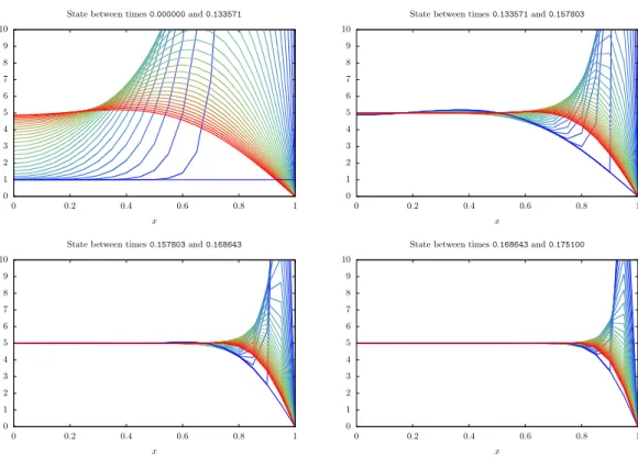
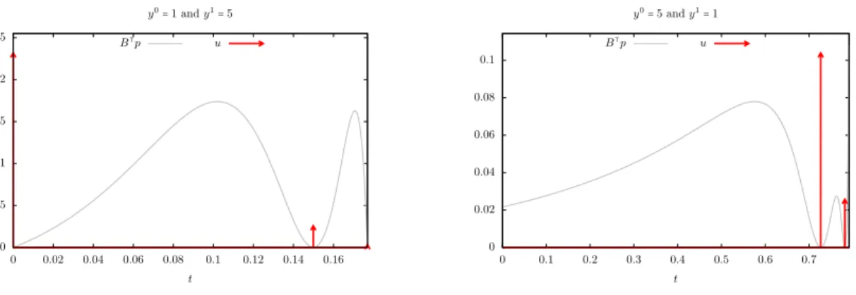
obtained from Proposition 7. The control and state trajectories are displayed on Figures 1 to 3. On Figure 1, we also plot B⊺_p(t), with p(t) the adjoint state obtained from IpOpt and we observe, as

expected from Proposition 3 that the Dirac masses are located at the times t such that B⊺_p(t) = 0.

On Figure 1, we observe that the minimal time control is the sum of 10 Dirac masses.

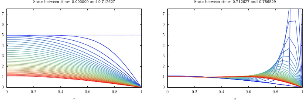
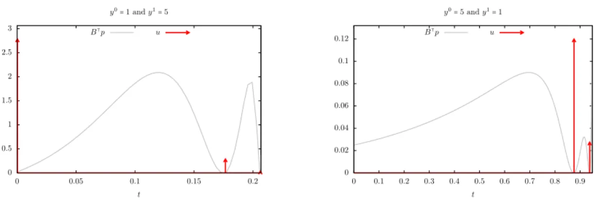
From y0≡ 5 to y1≡ 1. We set y0= (5, . . . , 5)⊺∈ IRn (with n= 20) and y1= (1, . . . , 1)⊺∈ IRn.

First of all, we numerically evaluate the constraint on the minimal time given in Proposition 7, to obtainTU(y

0_{, y}1_{) ⩾ 0.6613.}

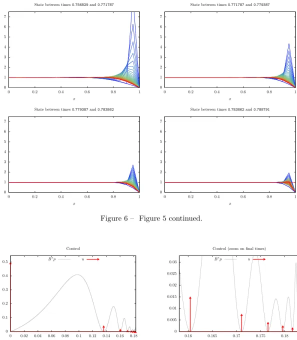
obtained from Proposition 7. The control and state trajectories are displayed on Figures 4 to 6. As in the previous example, we also plot, on Figure 4, B⊺_p(t), with p(t) the adjoint state obtained

from IpOpt and similarly, we observe that the minimal time control u computed by IpOpt is supported by the time instants where B⊺_p(t) = 0. On Figure 4, we observe that the minimal time

control is the sum of 7 Dirac masses.

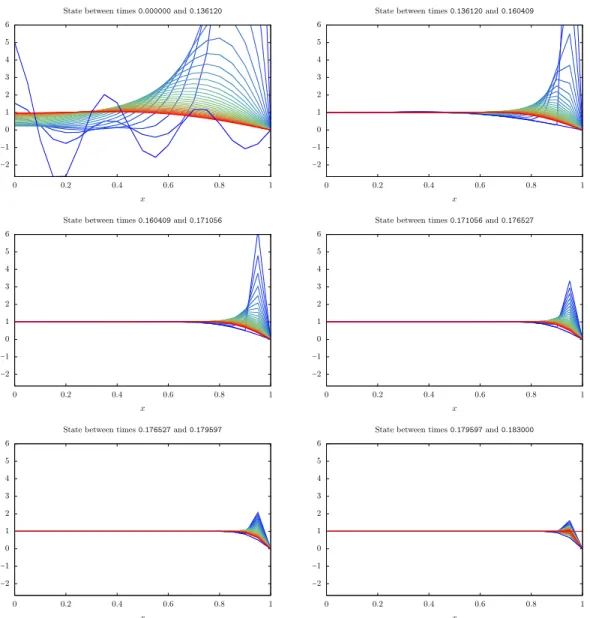
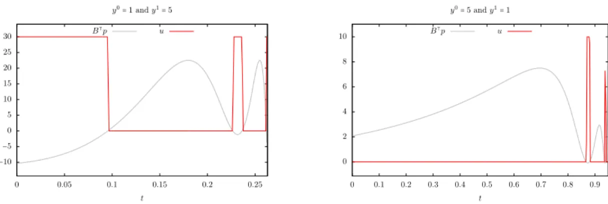
From y0_{(x) = 5 cos(11πx/2)/(4x + 1) to y}1 _{≡ 1. Let f(x) = 5 cos(11πx/2)/(4x + 1), we set}

y0 _{= (f(0), f(1/n), . . . , f((n − 1)/n))}⊺

∈ IRn _{(with n}

= 20) and y1 _{= (1, . . . , 1)}⊺ ∈ IRn. First of

all, we numerically evaluate the constraint on the minimal time given in Proposition 7, to obtain TU(y

0_{, y}1_{) ⩾ 0.0939.}

obtained from Proposition 7. The control and state trajectories are displayed on Figures 7 and 8.As in the previous examples, we also plot, on Figure 7, B⊺_p(t), with p(t) the adjoint state obtained

from IpOpt and similarly, we observe that the minimal time control u computed by IpOpt is supported by the time instants where B⊺_p(t) = 0. On Figure 7, we observe that the minimal time

(10)

0 0.5 1 1.5 2 0 0.02 0.04 0.06 0.08 0.1 0.12 0.14 0.16 0.18 t Control B⊺_p _u 0 0.02 0.04 0.06 0.08 0.1 0.12 0.14 0.16 0.155 0.16 0.165 0.17 0.175 0.18 0.185 t

Control (zoom on final times)

B⊺_p _u

Figure 1 – Minimal time control evolution in order to steer y0_{≡ 1 to y}1 _{≡ 5. The minimal time}

computed is TU(y

0_{, y}1_{) ≃ 0.186799. Dirac impulses are represented by arrows. On this figure,}

we also plot B⊺_p(t), with p(t) the adjoint state obtained from IpOpt. The corresponding state

trajectory is given in Figures 2 and 3.

0 1 2 3 4 5 6 7 8 9 10 0 0.2 0.4 0.6 0.8 1 x

State between times 0.000000 and 0.133571

0 1 2 3 4 5 6 7 8 9 10 0 0.2 0.4 0.6 0.8 1 x

Figure 2 – Evolution of the state between two Dirac impulses. The corresponding control required to steer y0_{≡ 1 to y}1_{≡ 5 is given in Figure 1 and the minimal time computed is T}

U(y

0_{, y}1_{) ≃ 0.186799.}

The color of the state goes from blue (for the initial time instant) to red (for the final time instant). (See Figure 3 for the final times.)

(11)

0 1 2 3 4 5 6 7 8 9 10 0 0.2 0.4 0.6 0.8 1 x

Figure 3 – Figure 2 continued.

0 0.01 0.02 0.03 0.04 0.05 0.06 0.07 0.08 0.09 0 0.1 0.2 0.3 0.4 0.5 0.6 0.7 t Control B⊺_p _u 0 0.005 0.01 0.015 0.02 0.772 0.774 0.776 0.778 0.78 0.782 0.784 0.786 0.788 t

B⊺_p _u

Figure 4 – Minimal time control evolution in order to steer y0_{≡ 5 to y}1 _{≡ 1. The minimal time}

computed isTU(y

0_{, y}1_{) ≃ 0.788791. Dirac impulses are represented by arrows. On this figure, we}

also plot a multiple of B⊺_p(t), with p(t) the adjoint state obtained from IpOpt. The corresponding

state trajectory is given in Figures 5 and 6.

0 1 2 3 4 5 6 7 0 0.2 0.4 0.6 0.8 1 x

Figure 5 – Evolution of the state between two Dirac impulses. The corresponding control required to steer y0_{≡ 5 to y}1_{≡ 1 is given in Figure 4 and the minimal time computed is T}

U(y

0_{, y}1_{) ≃ 0.788791.}

The color of the state goes from blue (for the initial time instant) to red (for the final time instant). (See Figure 6 for the final times.)

(12)

0 1 2 3 4 5 6 7 0 0.2 0.4 0.6 0.8 1 x

Figure 6 – Figure 5 continued.

0 0.1 0.2 0.3 0.4 0.5 0 0.02 0.04 0.06 0.08 0.1 0.12 0.14 0.16 0.18 t Control B⊺_p _u 0 0.005 0.01 0.015 0.02 0.025 0.03 0.16 0.165 0.17 0.175 0.18 t

B⊺_p _u

Figure 7 – Minimal time control evolution in order to steer y0_{(x) = 5 cos(11πx/2)/(4x + 1) to}

y1_{≡ 1. The minimal time computed is T} U(y

0_{, y}1_{) ≃ 0.183000. Dirac impulses are represented by}

arrows. On this figure, we also plot a multiple of B⊺_p(t), with p(t) the adjoint state obtained from

(13)

−2 −1 0 1 2 3 4 5 6 0 0.2 0.4 0.6 0.8 1 x

Figure 8 – Evolution of the state between two Dirac impulses. The corresponding control required to steer y0_{(x) = 5 cos(11πx/2)/(4x+1) to y}1_{≡ 1 is given in Figure 7 and the minimal time computed}

isTU(y

0_{, y}1_{) ≃ 0.183000. The color of the state goes from blue (for the initial time instant) to red}

(for the final time instant).

3 Numerical approximation of time optimal controls

In Section 2, we present some numerical simulations. The simulations have been performed by min-imizing the minimization problem (2.2) or(2.3). This has been possible because, we know exactly the eigenvalues and eigenvectors of A⊺. In a general situation, the computation of eigenvalues and

eigenvector is in itself a problem. Let us in addition mention that if the dimension of the matrix is large, solving the minimization problem (2.2) directly is hard. This is mainly due to the presence of exponentials in the constraints.

(14)

In order to overcome these facts, let us present here some other ways of numerically finding the minimal time and the time optimal control. We have tried all the other approaches proposed below. However, it seems that the method presented in Section 2 is the most efficient, in terms of computational time and result quality, for the discretized heat equation. Having a convergence proof for the numerical methods presented here is pointed in Open problem 9. Note that the construction of an efficient numerical method is also related to a better understanding of the adjoint problem, as pointed in Open problem 8.

Recall that it is possible to have TM < TU. We thus present in two different paragraphs the

methods which are designed for obtaining the timeTU and the one designed for obtainingTM.

Obtaining the time TM.

Numerical method 1 (Momentum approach). This approached is based on the expression of optimal control problem in the basis generated by the eigenvectors of A has been explained in Section 2. Note that this approach is only applicable in the cases where A is a diagonalisable matrix.

Numerical method 2 (Total discretization). This approach is used to find the minimal time TM(y

0_{, y}1_{) and a control in time T} M(y

0_{, y}1_{). Recall that if a nonnegative measure control exist in}

timeTM(y

0_{, y}1_{), then it is the sum of at most N Dirac masses (N ⩽ ⌊(n+1)/2⌋ when the matrix A}

satisfies the Assumption (H.2)). We thus pick N > 0 large enough, and define 0 = t0 ⩽ t1 ⩽ ⋅ ⋅ ⋅ ⩽

tN ⩽ T = tN +1, t1, . . . , tN being the time instants where a Dirac impulse can occur. Between times

tk and tk+1, the control is 0 and solution is given by y(t) = yk(t − tk), with yk solution of

˙

yk(t) = Ayk(t) (t ∈ (0, tk+1− tk)), (3.1)

with initial condition given below. For every k∈ {1, . . . , N +1} we have yk(0) = yk−1(tk−tk−1)+γkB

for some γk⩾ 0. At initial and final times we have y0(0) = y0 and yN(T − tN) = y1. Notice that if

a Dirac impulse occurs at the initial or final time, we will have t1= 0 or tN = T respectively.

Let us define τk = tk+1− tk for every k∈ {0, . . . , N}, we have T = ∑Nk=0τk and yk(τk) = eτkAyk(0).

We also set y0

k= yk(0). The minimization problem is then

min

N

∑

k=0

τk (3.2a)

subject to the constraints: 0⩽ τk and yk0∈ IR n (k ∈ {0, . . . , N}), (3.2b) y₀0= y0 and y1= eτNAy0_N, (3.2c) PB(yk+10 − e τkA_y0 k) ⩾ 0 and P ⊥ B(y 0 k+1− e τkA_y0 k) = 0 (k ∈ {0, . . . , N − 1}), (3.2d)

where PB (respectively PB⊥) is an orthogonal projector on Ran B (respectively(Ran B) ⊥).

The constraint (3.2c) ensures that the initial condition y(0) = y0_{and the final condition y(T) = y}1

are satisfied, and the constraint (3.2d) ensures the existence of some γk ⩾ 0 such that yk+1(0) =

yk(τk) + γkB.

In order to perform numerical simulations, one needs to compute eτkA. To this end, it is possible

(15)

Numerical method 3(Using a time reparametrization). As we will see in § 5.2.1, the minimal timeTM(y

0_{, y}1_{) is obtained through the minimization problem:}

min _∫ S 0 w(s) ds S⩾ 0, w(s) ∈ [0, 1] (s ∈ [0, S]), z(S) = y1, with z the solution of

⎧⎪⎪ ⎨⎪⎪ ⎩ ˙ z(s) = w(s)Az(s) + B(1 − w(s)) (s ∈ [0, S]), z(0) = y0_. (3.3) We then haveTM(y 0 , y1) = ∫ S 0 w(s) ds.

The interest of this approach is that now, the new control w is uniformly bounded and any classical method to find the corresponding optimal control problem can be used. As explained in § 5.2.1, under this change of variables, the time instances s in which w(s) = 0 corresponds to the presence of active Dirac masses while w(s) > 0 corresponds to a bounded L∞ control, the limit

being w(s) = 1, corresponding to the absence of control action.

As far as we know, this numerical method is the only one proposed in this article that can be adapted to nonlinear control problems. We refer to [9, 21, 4, 15] for the adaptation of the time reparametrization for nonlinear control systems.

This method can also be adapted to find the minimal timeTU(y

0_{, y}1_{), see Numerical method 6.}

Numerical method 4 (Approximation by a sequence of nonnegative controls of minimal L1

norm). For additional details about this method, we refer to Appendix C. Assume that y1_{∈ S}∗

+, and that 0< TM(y

0_{, y}1_{) < ∞, then for every time T > T} M(y 0_{, y}1_{) (recall} thatTU(y 0_{, y}1_{) = T} M(y 0_{, y}1_{) when y}1_{∈ S}∗

+), there exist a control u∈ M+(T) steering y

0 _{to y}1 _in

time T . In particular, there exist a control of minimal measure. Note also that for every non-negative time T < TM(y

0_{, y}1_{), there does not exist a control in M}

+(T) steering y

0_{to y}1_{in time T .}

The idea is then to find the minimal time T such that the optimal control problem inf ∥u∥M([0,T ])

u∈ M+(T),

y1− eT Ay0= ΦTu

(3.4)

admits a solution.

The dual problem of (3.4) is:

inf ⟨eT Ay0− y1, p1⟩ p1_{∈ IR}n_,

B⊺_e(T −t)A⊺_p1⩽ 1 (t ∈ [0, T]) .

(3.5)

Using weak duality results, one can show that if the infimum of the minimization problem given by (3.5) is−∞, then, there does not exist a control in M+(T) steering y

0_{to y}1_{in time T (i.e., T} _<

TM(y

0_{, y}1_{)). By strong duality result, one can also show that for T > T} M(y

0_{, y}1_{), the minimization}

problem (3.5) admits a minimum. Reciprocally, using first order optimality conditions, we can prove that if the minimization problem (3.5) admits a minimum, then there exist a control u∈ M+(T) steering y

0 _{to y}1 _{in time T and this control is the sum of a finite number of Dirac masses.}

It is possible to use these facts to build an algorithm in order to find an approximation of the minimal timeTM(y

0_{, y}1_{) (see Algorithm 1). This algorithm, is based on a dichotomy approach,}

(16)

Algorithm 1Approximation ofTM(y 0_{, y}1_). Require: ε> 0 Require: y0∈ IRn, y1∈ S∗ + and TM(y 0_{, y}1_{) < ∞} Ensure: 0⩽ T − TM(y 0_{, y}1_{) < ε} {Test ifTM(y 0_{, y}1_{) = 0:}} T0← 0

if (3.5) (with T = 0) admits a minimizer then return T = 0

else T0← 0

{Find T1> 0 such that (3.5) (with T = T1) admits a minimizer:}

T1← 1

while (3.5) (with T = T1) does not admit a minimizer do

T1← T1+ 1

end while end if

{We now have T0⩽ TM(y

0_{, y}1_{) ⩽ T} 1.}

{Do the dichotomy procedure:} while T1− T0⩾ ε do

if (3.5) (with T = (T0+ T1)/2) admits a minimizer then

T1← (T0+ T1)/2 else T0← (T0+ T1)/2 end if end while return T = T1

Remark 9. Note that the minimization problem (3.5) is a linear programming problem. To test whether the minimum is achieved or not, one can use the simplex algorithm, see for instance [10]. Furthermore, the linear inequality B⊺_e(T −t)A⊺_p1 ⩽ 1 for every t ∈ [0, T], in (3.5), is numerically

teated as B⊺_e(T −ti)A⊺_p1⩽ 1 for every i ∈ {0, . . . , n

T}, with ti= iT/nT and with nT ∈ IN∗ large.

Note also that it is possible to use the numerical strategy proposed in [17, 18] in order to find the control of minimal measure. This strategy would avoid the usage of the simplex method. More precisely, it might be possible to adapt the work done in [17, 18] to find a nonnegative control of minimal L1_{-norm such that y}_{(T) (the controlled state at the final time) is at distance ε from}

the target y1_{. The algorithm proposed in [17, 18], is based on a greedy algorithm, and might be}

efficient when T> TM(y

0_{, y}1_{). However, there is still some work to do so that for T < T} M(y

0_{, y}1_),

the algorithm answers that no minimizer exist. ∎ Remark 10. We have assumed here that y1∈ S∗

+. But, probably, it is sufficient to assume that for

every time T> TM(y

0_{, y}1_{), there exist a control u ∈ M}

+(T) steering y

0 _{to y}1_{in time T . However,}

without the assumption y1_{∈ S}∗

+, we are currently unable to prove the strong duality result (see

Remark C.3 for more details). ∎

Remark 11. On one hand, if we are able to pass to the limit T → TM, we would obtain the

existence of an adjoint state p such that B⊺_p⩽ 1 and such that the Dirac masses are located in the

set of times t such that B⊺_p(t) = 1.

On the other hand, Corollary 5.2.2 ensures the existence of an adjoint p such that B⊺_p⩾ 0 and

(17)

This means that at the minimal time, there would exist two different adjoints states leading to a control at the minimal timeTM. When the matrix A satisfies the assumption (H.2), the minimal

time control is unique, thus these two adjoints states shall lead to the same control. The relation between these two adjoint is not understood and postponed in Open problem 8. ∎

Obtaining the time TU.

Numerical method 5 (Approximation by bang-bang controls). Note that this approach, based on the approximation result given in Proposition 5.3.1, has already been used in [19]. Let us also point out that the minimization problem (2.3) is adapted for finding the minimal timeTM(y

0_{, y}1₎

and in the numerical simulations given in Section 2, we use the fact that y1 _{∈ S}∗

+, and hence

TM(y

0_{, y}1_{) = T} U(y

0_{, y}1_{). However, as pointed out in § 5.1.3, there might exist y}0 _{and y}1 _{such that}

TM(y

0_{, y}1_{) < T} U(y

0_{, y}1_{). In this situation, a way to find T} U(y

0_{, y}1_{) is to solve, for M > 0, the}

minimization problem: min T

T > 0,

0⩽ u(t) ⩽ M (t ∈ (0, T) a.e.),

y(0) = y0 _{and y}_{(T) = y}1_, _{with y solution of (1.1)}

(3.6)

and let M goes to∞. We refer to Section 5.3 for more results of the convergence of the minimizer of this minimization problem as M→ ∞. The interest of this approach is that now, the control u is uniformly bounded and any classical method to find the corresponding optimal control problem can be used.

Numerical method 6 (Using a time reparametrization - second version). The idea used in Numerical method 3 can also be used to design a numerical method aiming to find the minimal timeTU. In fact as explained in Numerical method 3, w= 0 correspond to Dirac masses. In order

to avoid Dirac masses, we fix ε∈ (0, 1) and solve the minimization problem: min _∫ S 0 w(s) ds S⩾ 0, w(s) ∈ [ε, 1] (s ∈ [0, S]), z(S) = y1_, _{with z the solution of}

⎧⎪⎪ ⎨⎪⎪ ⎩ ˙ z(s) = w(s)Az(s) + B(1 − w(s)) (s ∈ [0, S]), z(0) = y0. (3.7)

In this problem, the constraint w(s) ⩾ ε avoids the presence of Dirac masses and as ε → 0, we will recover the minimal timeTU(y

0_{, y}1_{). In fact, the constraint w(s) ⩾ ε ensures that in the original}

time scale, the control u is uniformly bounded by(1 − ε)/ε.

Numerical comparison between the different approaches.

In order to compare the different numerical approaches proposed in the previous paragraphs, we consider the system (1.1) with matrices A and B given by (1.4), with n= 5. For this system, we consider the case y0 _{≡ 1 and y}1_{≡ 5, and the case y}0 _{≡ 5 and y}1_{≡ 1. Note that we expect to}

have no more that N = ⌊(n + 1)/2⌋ = 3 Dirac masses involved in the minimal time control. Since y1 _{∈ S}∗

+, we have TU(y

0_{, y}1_{) = T} M(y

0_{, y}1_{) and the control at the minimal time is unique. Hence,}

all the numerical methods proposed shall, up to numerical errors, give the same time and optimal control.

(18)

Note that for Numerical methods 3, 5 and 6, we end up with an optimal control problem written in its classical form. To computationally solve these problems, we used the total discretization method introduced in [27, Part 2, § 9.II.1], combined with the Crank-Nicolson method. The number of time discretization points is precised below.

• For Numerical method 1, we allow N= 3 Dirac masses. • For Numerical method 2, in order to compute eτkA_y0

k, appearing in (3.2d), we solve (3.1), with

initial condition y0

k, using the Crank-Nicolson method with nt= 100 discretization points.

Note that this means that on the full time interval, we have 400 discretization points in time. Since we observe that a Dirac mass is located close to the final time, this in fact means that we have, in fact, no more than 300 effective discretization points in time (the last τk

in (3.2) is almost 0). This explains why we use 300 discretization points in time for Numerical methods 4 and 5.

• For Numerical method 3, in the case y0_{≡ 1 and y}1_{≡ 5 (respectively y}0_{≡ 5 and y}1_{≡ 1), we use}

nt= 900 (respectively nt= 500) discretization points in time in the Crank-Nicolson method.

This difference between the number of discretization points, is due to the fact that the system is discretized over[0, S], where S is in fact the sum of the minimal time TU(y

0_{, y}1₎

and measure of the optimal control. When y0_{≡ 1 and y}1_{≡ 5 (respectively y}0_{≡ 5 and y}1_{≡ 1),}

after computation, we obtain S≃ 3.321291 (respectively S ≃ 1.098819).

• For Numerical method 4, we rewrite the constraint B⊺_e(T −t)A⊺_p1⩽ 1 (for every t ∈ [0, T]),

appearing in (3.5), as⟨etA_{B, p}1_{⟩ ⩽ 1 (for every t ∈ [0, T]) and we compute the values of e}tA_B

using Crank-Nicolson method with nt= 300 discretization points. Furthermore, the

param-eter ε appearing in Algorithm 1 is fixed to 10−4_{, and the solution of the linear optimization}

problem is computed with a simplex algorithm.

• For Numerical method 5, we use nt= 300 discretization points in the Crank-Nicolson method.

Furthermore, the value of M is fixed to 10 for the case y0_{≡ 1 and y}1_{≡ 5, and to 30 for the}

case y0_{≡ 5 and y}1_{≡ 1. We use M = 10 (for the first case) and M = 30 (for the second case)}

simply for graphical reasons.

• For Numerical method 6, we use here the same number of discretization points as for Numer-ical method 3 in the Crank-Nicolson method. As for NumerNumer-ical method 5, we use ε= 1/10 (respectively ε= 1/30) in the case y0_{≡ 1 and y}1_{≡ 5 (respectively y}0_{≡ 5 and y}1_{≡ 1).}

In practice, we use IpOpt and AMPL to numerically solve the optimal problems given in Numerical methods 1 to 3, 5 and 6, and to solve the linear programming problem appearing in Numerical method 4, we use the linpro routine (see [5]) of Scilab.

Corresponding results are plotted on Figures 9 to 14 and the computed minimal times are gather in Table 2. We also plot on these figures the corresponding adjoint states. We can then see, as expected, that for Numerical methods 1 to 4, there exist an adjoint state p such that the optimal control is active when B⊺_p⩽ 0 and null for all the other times. For Numerical method 4, we can

also see that there exist an adjoint state p such that the optimal control is active when B⊺_p= 1.

Understanding the relation between these two adjoint states is the goal of Open problem 8 below. We observe on Table 2 that the times obtained for Numerical methods 5 and 6 are similar and greater than the times obtained for the other numerical methods. This fact was expected, since in this case, we are looking for a bounded control in L∞, hence, the time obtained has to

be greater than TU(y

0_{, y}1_{) (the time which shall be obtained with Numerical methods 1 to 4).}

We also observe that the times obtained for Numerical methods 1 and 4 are similar and lower than the times obtained for Numerical methods 2 and 3. We do not know how to explain the gap

(19)

between these two times. This can be due to the fact that we are solving a nonlinear minimization problem and that for Numerical methods 2 and 3, we only find a local minimum. Note also that the convergence of the optimization algorithm is really dependent on the initialization point. To compute the above results, we progressively increase the parameters n and ntup to their desired

values and between two increments of the parameters, we initialized the optimization algorithm with the previously computed result.

Numerical method 1 2 3 4 5 6

y0_{≡ 1 and y}1_{≡ 5}

0.185024 0.201834 0.206753 0.176994 0.263030 0.265068 y0≡ 5 and y1≡ 1 0.793984 0.873111 0.948933 0.791016 0.949745 0.949479 Table 2 – Minimal time TU(y

0_{, y}1_{) computed with Numerical methods 1 to 6 for the case y}0 _≡

1and y1 _{≡ 5 and y}0 _{≡ 5 and y}1 _{≡ 1. More details on the parameters used for these numerical}

methods are given in the last paragraph of Section 3.

0 0.5 1 1.5 2 2.5 0 0.02 0.04 0.06 0.08 0.1 0.12 0.14 0.16 t y0_{= 1 and y}1_{= 5} B⊺_p _u 0 0.02 0.04 0.06 0.08 0.1 0 0.1 0.2 0.3 0.4 0.5 0.6 0.7 t y0_{= 5 and y}1_{= 1} B⊺_p _u

Figure 9 – Results for Numerical method 1. See Table 2 for the corresponding minimal times.

0 0.5 1 1.5 2 2.5 3 0 0.05 0.1 0.15 0.2 t y0_{= 1 and y}1_{= 5} B⊺_p _u 0 0.02 0.04 0.06 0.08 0.1 0.12 0 0.1 0.2 0.3 0.4 0.5 0.6 0.7 0.8 0.9 t y0_{= 5 and y}1_{= 1} B⊺_p _u

(20)

0 0.5 1 1.5 2 2.5 3 0 0.05 0.1 0.15 0.2 t y0_{= 1 and y}1_{= 5} B⊺_p _u 0 0.02 0.04 0.06 0.08 0.1 0.12 0 0.1 0.2 0.3 0.4 0.5 0.6 0.7 0.8 0.9 t y0_{= 5 and y}1_{= 1} B⊺_p _u

Figure 11 – Results for Numerical method 3. See Table 2 for the corresponding minimal times. Recall that here, the dynamical system is rescaled in time, and the new control w belongs to[0, 1]. The figures here are displayed in the original time and a posttreatment of the result has been done to observe Dirac masses.

−0.5 0 0.5 1 1.5 2 0 0.02 0.04 0.06 0.08 0.1 0.12 0.14 0.16 t y0_{= 1 and y}1_{= 5} u B⊺_p− 1 −0.8 −0.6 −0.4 −0.2 0 0 0.1 0.2 0.3 0.4 0.5 0.6 0.7 t y0_{= 5 and y}1_{= 1} u B⊺_p_{− 1} −0.002 0 0.002 0.004 0.006 0.008 0.01 0.012 0.014 0.71 0.72 0.73 0.74 0.75 0.76 0.77 0.78 0.79

t(Zoom on final times.) y0_{= 5 and y}1_{= 1}

u B⊺_p_{− 1}

Figure 12 – Results for Numerical method 4. Note that here, instead of plotting B⊺_p, we plot

(21)

−10 −5 0 5 10 15 20 25 30 0 0.05 0.1 0.15 0.2 0.25 t y0_{= 1 and y}1_{= 5} B⊺_p _u 0 2 4 6 8 10 0 0.1 0.2 0.3 0.4 0.5 0.6 0.7 0.8 0.9 t y0_{= 5 and y}1_{= 1} B⊺_p _u

Figure 13 – Results for Numerical method 5. See Table 2 for the corresponding minimal times. Note that in both cases, we expect that the control takes its values in{0, M} for almost every time. But this fact is note observed on the right figure (M = 10 in the case y0 _{= 5 and y}1 _{= 1).}

However, by increasing the number of time discretization points, we will recover this saturation property. −10 −5 0 5 10 15 20 25 30 0 0.05 0.1 0.15 0.2 0.25 t y0_{= 1 and y}1_{= 5} B⊺_p _u 0 2 4 6 8 0 0.1 0.2 0.3 0.4 0.5 0.6 0.7 0.8 0.9 t y0_{= 5 and y}1_{= 1} B⊺_p _u

Figure 14 – Results for Numerical method 6. See Table 2 for the corresponding minimal times. Recall that in this case, the control is bounded by (1/ε − 1)/ε, and we had chosen ε = 1/30 (respectively ε= 1/10) for y0_{= 1 and y}1 _{= 5 (respectively y}0 _{= 5 and y}1 _{= 1). Recall also that as}

for Figure 11, the dynamical system is rescaled in time, and the new control w belongs to[ε, 1]. The figures here are displayed in the original time scale.

4 Further comments and open questions

In this paper, we show that controlling with nonnegative controls a finite-dimensional linear au-tonomous control system ˙y= Ay + Bu satisfying the Kalman condition requires a positive minimal time as soon as the difference between the initial state and target state does not belong to Ran B. When A admits at least one real eigenvalue (and when the target is reachable with nonnegative Radon measure control, i.e.,TM(y

0_{, y}1_{) < ∞), there exists a minimal time nonnegative control in}

the space of Radon measures and this control is a linear combination with nonnegative coefficients of a finite number of Dirac impulses. Without this spectral assumption the conclusion may fail. In addition, when all eigenvalues of A are real, the number of Dirac masses involved in the time

(22)

optimal control is no more than half of the space dimension and the time optimal control is unique. Let us mention several open questions and propose some other numerical strategies aiming to find the minimal controllability time.

Open problem 1 (Nonnegative vectorial controls). In this paper, we only study the case of a nonnegative scalar control. The same question with a control u∈ IRm

+ (with m⩾ 2) is not presented

here. However, it shall be easy to adapt the proof given for the scalar case to the m-dimensional control case. This extension is, in particular, relevant for discretized versions of higher dimensional heat equation or 1D heat equation with controls at both ends.

Note that when controlling the discretized version of a 1D heat equation with Dirichlet controls at both ends, we can use the symmetry properties already discussed in [19] to come back (when the initial state and target states are both symmetric) to the problem present work.

Open problem 2(Do we haveTU(y

0_{, y}1_{) = T} M(y

0_{, y}1_{)). We have shown that if the target state}

is a steady-state then the minimal controllability time for nonnegative Radon measure controls coincides with the one for nonnegative L∞-controls. In general a gap may occur, as exemplified

in Remark 5.1.9. But, there is no clear picture for the existence of a gap, and we refer to [21] for further results in this direction.

Open problem 3(Existence of a minimal time control). When no eigenvalue of A is real, we are not able to show that a minimal time control in the space of nonnegative Radon measure exists. As shown in Remark 5.1.8, the answer to this question might be negative in some situations. The difficulty encountered in order to solve this problem is due to the lack of uniform bound on the norm of the controls in times greater than the minimal time.

Open problem 4 (Number of Dirac impulses in the minimal time control). We show in Corol-lary 5.2.2 that if a minimal time control exist, then this control is a linear combination with non-negative coefficients of a finite number of Dirac impulses. But we do not have an estimate on the number of impulses. We also show in Proposition 5.2.5 that under the stronger assumption (H.2) (all eigenvalues of A are real), we have an explicit bound on the number of Dirac impulses. Is it possible to obtain an upper bound on the number of Dirac masses involved in the time optimal control without the assumption (H.2)?

Open problem 5(Uniqueness of the minimal time control). The uniqueness of the minimal time control (if it exists) remains open when at least one of the eigenvalues of A is not real. If we aim to follow the proof of Proposition 5.2.5, we need to show that any minimal time control consists of at most⌊(n + 1)/2⌋ Dirac impulses. Consequently, this question might also be related to the Open problem 4.

Open problem 6(Localization of the Dirac masses). We only know under the assumption (H.1) that a finite number of Dirac masses are involved in any time optimal control. Finding their location passes through an optimization algorithm, and we do not know a priori repartition of the Dirac masses. In particular, for the discretized heat equation, it seems that the localization of the Dirac masses and their amplitude is rather organized (see Figures 1, 4 and 7).

Open problem 7(Convergence speed of the minimal controllability time with bounded L∞-controls

to the one with unbounded controls). We have proved that the minimal time for the minimal time control problem under the additional control constraint 0⩽ u(t) ⩽ M converges to the minimal time as M→ +∞. Obtaining convergence rates is an interesting problem and the answer to this question would be helpful for numerical simulations. Some key arguments may be found in [24, 25, 26]. Open problem 8(Obtaining the minimal time control through the adjoint). In classical optimal control problems, the optimal control is given in function of the adjoint. This means that there

(23)

exists a function f such that u(t) = f(B⊺_p(t)), where p is solution of ˙p = −A⊺_pwith the terminal

condition p(T) = p1_{∈ IR}n_{. At this level, this structure is badly understood.}

In Appendix C, we have tried, without success, to obtain the optimal control by computing the control of L1_{-minimal norm in time T} _{> T}

M and passing to the limit as T → TM. For T > TM,

the control of minimal L1_{-norm is a sum of Dirac impulses and these Dirac impulses are located}

on a level set of the adjoint observations (more precisely on the set of time t∈ [0, T] such that B⊺_p(t) = 1). However, we have shown that the terminal condition p1minimizes a linear cost and is

subject to a unilateral linear constraint. This fact is not enough to obtain compactness on p1_and

does not allow us to pass to the limit as T → TM. In addition, once the control is characterized

by the adjoint state, an optimal control is given by an adjoint minimizing some functional. The existence of such minimum is usually related to an observability inequality. In Appendix C, for T> TM, we do not know how to interpret the existence of a minimum of (C.3) for the dual problem

in terms of an observability inequality.

Finally, in the proof of Proposition 5.2.5, we use the adjoint state related to the minimization problem (5.6). Similarly, this leads to an adjoint state p(t) such that B⊺_p(t) is of constant sign

and such that the control is active only at the time instants such that B⊺_p(t) = 0.

The understanding of the relations between these two adjoint states remains open.

Open problem 9 (Numerical approximation of the time optimal control). Nothing ensures the convergence of the numerical method proposed in Sections 2 and 3, except for the Numerical method 4, which is based on Algorithm 1 (see also Appendix C), where we only consider the controllability to a positive steady state target.

This lack of convergence proof is mainly due to the fact that we are solving a nonlinear control problem. Having some efficient and general numerical method ensuring that the computed control is at some distance ε from the real control is as far as we know an open problem. This question is also related to the previous one (Obtaining the minimal time control through the adjoint), since it is usually more efficient to minimize a cost function related to the adjoint variable, than looking directly for an optimal control. Note also that the main question is the time location of the Dirac masses. In fact, once these locations are found, the amplitude of the Dirac masses is obtained by solving a linear system.

Open problem 10 (Limit as n→ +∞ of the discretized heat equation). One of the issues of this paper concerns the study of the controllability of the discretized heat equation with nonnegative Dirichlet controls. An open issue is the convergence of the obtained results as n→ +∞. In partic-ular, we would expect that for the heat system described by (1.3) the minimal time nonnegative control is a linear combination with nonnegative coefficients of a countable number of Dirac im-pulses. If this is true, we would also aim to know how these Dirac impulses are distributed over the time interval. The answer to this question may require a better understanding of the adjoint system.

5 Proof of the main results

5.1 Preliminaries

5.1.1 Accessibility conditions

In this paragraph, we do not aim to give an exhaustive description of the accessible points from some y0_{. For this question, we refer to [13, 14]. Here we only recall that a steady-state}

connected-ness assumption ensures controllability in large enough time.

Since B is a vector of IRn_{and since the pair}_{(A, B) satisfies the Kalman rank condition, the set}

of steady-states is a subspace of IRn _{of dimension one. Let us point out that}_S∗

(24)

or the empty set. In fact, it is easy to see thatS∗

+ is empty when B∉ Ran A and a half-line when

B∈ Ran A.

The next result can be obtained with the quasi-static strategy and easily follows from small-time local controllability combined with a compactness argument. We refer to [7, 8, 22] for more details. Proposition 5.1.1. Assume S∗ + ≠ ∅. Let ¯y 0_{, ¯}_y1 _{∈ S}∗ +, let ¯u 0_{, ¯}_u1 _{∈ IR}∗

+ their associated

steady-state controls (i.e., A¯yi_{+ B¯u}i _{= 0 for i ∈ {0, 1}) and let µ = min(¯u}0_{, ¯}_u1_{) > 0. Then there exist}

ρ= ρ(µ) > 0 and a positive time T ⩽ (3 + ∣¯y1− ¯y0∣/2ρ) µ such that for every y0 ∈ B(¯y0, ρ) and every y1 _{∈ B(¯y}1_{, ρ}_{), there exists a control u ∈ U}

+(T) such that the solution of (1.1) with initial

condition y0 _{and control u reaches y}1 _{at time T .}

Proof. Let us recall that a linear control system is small-time locally controllable around any steady-state(¯y, ¯u) ∈ IRn_{× IR, i.e. (see [6, Definition 3.2 p. 125]), for every ε > 0, there exist ρ(ε) > 0}

such that for every y0 _{and every y}1_{in B}_{(¯y, ρ(ε)), there exists a measurable function u ∶ [0, ε] → IR}

such that∣u(t) − ¯u∣ ⩽ ε for every t ∈ [0, ε] and the solution of (1.1) starting from y0 _{reaches y}1 _at

time ε. Note that for linear control systems, ρ can be chosen independent of ¯y.

In particular, choosing ε= µ (and ρ = ρ(µ)), for every steady-sate (¯y, ¯u), with ¯u > µ, and for every y0_{and y}1 _{in B}_{(¯y, ρ), there exists a control u ∈ U}

+(µ) such that the solution of (1.1) starting

from y0_{reaches y}1 _{at time µ.}

To prove the statement of Proposition 5.1.1, we consider the sequence of points ˜

y0= y0, ˜y1= ¯y0+ (¯y1− ¯y0)α, . . . , ˜yN = ¯y0+ (2N − 1)(¯y1− ¯y0)α, ˜yN +1= y1, where α∈ IR+∗ and N ∈ IN are designed so that

• ˜yk _{and ˜y}k+1 _{belong to the ball of radius ρ centered on the steady-state point} _(˜yk_{+ ˜y}k+1_)/2

for every k∈ {1, . . . , N − 1};

• ˜y1_{belong to the ball of radius ρ centered on the steady-state point ¯y}0_;

• ˜yN _{belong to the ball of radius ρ centered on the steady-state point ¯y}1_.

These conditions lead to α< ρ ∣¯y1_−¯_y0∣ and 1 2(1 + 1 α− ρ α∣¯y1_−¯_y0∣) < N < 1 2(1 + 1 α+ ρ α∣¯y1_−¯_y0∣).

By construction, it is then easy to build a control inU+(µ) steering y

k _{to y}k+1 _{in time µ. Thus, by}

concatenation of these controls, we have build a control steering y0 _{to y}1 _{in a time T lower than} µ

2(1 + 1 α+

ρ

α∣¯y1_−¯_y0_∣) + 2µ. For the sake of readability, we illustrate this construction on Figure 15.

Taking the limit α→ ρ/∣¯y1_{− ¯y}0_{∣, we obtain the upper bound estimation on T.}

Proposition 5.1.2. Assume that all the eigenvalues of A has a negative real part. Let ¯y1 _∈

S∗

+ and let ¯u 1 _{∈ IR}∗

+ its associated steady-state control (i.e., A¯y

1_{+ B¯u}1 _{= 0). Then there exist}

ρ = ρ(¯u1) > 0 such that for every y0 ∈ IRn and y1 ∈ B(¯y1, ρ) there exists a positive time T ⩽ inf{t > 0 ∣ C(t) < ρ/∣¯y1− y0∣} + ¯u1, with C(t) = sup {∣etAz∣ ∣ z ∈ IRn,∣z∣ ⩽ 1}, and a control u ∈ U+(T) such that the solution of (1.1) with initial condition y

0_{and control u reaches y}1_{at time T .}

Proof. We use the dissipativity of the system. More precisely, taking the constant control u(t) = ¯u1_,

the solution of (1.1) with initial condition y0_{(and control u) exponentially converges to ¯y}1_{. More}

precisely, we have∣¯y1_{− y(t)∣ ⩽ C(t)∣¯y}1_{− y}0_∣.

We then use the small-time local controllability around the steady-state(¯y1_{, ¯}_u1_{). This means}

that there exist ρ= ρ(¯u1_{) > 0 such that for every y}0 _{and y}1 _{in B(¯y}1_{, ρ}_{), there exists a control}

u∈ U+(¯u

1_{) such that the solution of (1.1) starting from y}0 _{reaches y}1 _{at time ¯u}1_.

(25)

y0 y1 y1 (̃y1_{+ ̃y}2_{) /2} (̃y2_{+ ̃y}3_{) /2} ̃y2 ̃y3 y0 0 S∗₊ ̃y1

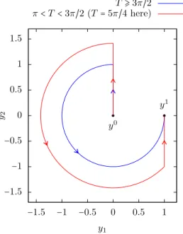
Figure 15 – State trajectory for the control built in the proof of Proposition 5.1.1.

Remark 5.1.3. In addition to the reachability condition, the Propositions 5.1.1 and 5.1.2 also give an upper bound on the reachability time. However, to explicitly know this bound, one needs to know the parameter ρ, which is not explicit. ∎ Lemma 5.1.4. AssumeS∗

+≠ ∅. Let y

0_{, y}1_{∈ IR}n _{and assume that y}0_{or y}1 _{belongs to}_S∗

+. Assume,

in addition, the existence of T > 0 such that y1 _{is reachable from y}0 _{in time T with a control in}

M+(T). Then for every τ ⩾ 0, y

1 _{is reachable from y}0 _{in time T}_{+ τ.}

The proof of this lemma is straightforward: a control in time T+τ is obtained by concatenation of a control in time T with the constant control ¯u associated to the steady-state y0 _{or y}1_.

Remark 5.1.5. As for Propositions 5.1.1 and 5.1.2, the condition y0 _{∈ S}∗ + or y

1 _{∈ S}∗

+ (in the

statement of Lemma 5.1.4) can be relaxed to yi _{∈ B(¯y}i_{, ρ}_{), with ¯y}i _{∈ S}∗

+ (for i= 0 or i = 1) and

ρ> 0 small enough (depending on τ and ¯y0 or ¯y1). To this end, we use small time controllability around the steady state ¯y0 _{or ¯y}1_. _∎

Remark 5.1.6. The result of Lemma 5.1.4 can be trivially extended to the problem of controlla-bility to trajectories. In fact, set ¯y is a solution of (1.1) with a nonnegative control ¯u∈ L∞(IR

+),

and set y0_{∈ IR}n_{. If there exists a time T and a control u}_{∈ U}

+(T) such that the solution y of (1.1),

with initial condition y0 _{and control u, satisfies y(T) = ¯y(T), then for every τ > 0, there exist a}

control uτ ∈ U+(T + τ) such that the solution y of (1.1), with initial condition y

0 _{and control u} τ

satisfies y(T + τ) = ¯y(T + τ). To this end, we only take, uτ(t) = u(t) for t ∈ (0, T), and uτ(t) = ¯u(t)

for t∈ (T, T + τ). ∎

5.1.2 Existence of a positive minimal controllability time and minimal time controls An important notion to define the minimal time is the accessible set with nonnegative controls

Acc+(T) = {ΦTu , u∈ U+(T)} .

The minimal controllability timeTU(y

0_{, y}1_{) defined by (1.5) is then}

TU(y

0_{, y}1_{) = inf {T > 0 ∣ y}1_{− e}T A_y0_{∈ Acc}

+(T)} (y

(26)

and by convention,TU(y

0_{, y}1_{) = +∞ when y}1_{is not accessible from y}0_{in any time, i.e., y}1_−eT A_y0_∉

Acc+(T) for every T > 0.

As explained in [20], for T > 0 small enough, Acc+(T) is isomorphic to the positive quadrant

of IRn_{. This ensures that whatever y}0_{∈ IR}n _{is, there always exists y}1_{∈ IR}n_{such that}

TU(y

0_{, y}1_{) > 0.}

The problem is to characterize this minimal control time and to determine whether there exists a control at the minimal time. Similarly to [19], it can be checked that the existence of a minimal controllability time is ensured in the set of Radon measures.

Proposition 5.1.7. Let y0 and y1 be two points of IRn such that 0⩽ TU(y

0_{, y}1_{) < +∞, i.e., y}1 _is

accessible from y0_{. Under Assumption (H.1), there exists a control u}_{∈ M} +(TU(y

0_{, y}1_{)) steering}

the system (1.1) from y0 _{to y}1 _{in time} _T U(y

0_{, y}1_).

The same result holds withTU(y

0_{, y}1_{) replaced with T} M(y

0_{, y}1_).

Proof. The argument is similar to the one used in [19]. We prove here this result in the case of L∞nonnegative controls. The same proof can be made for nonnegative Radon measure controls.

Let us denote TU = TU(y

0_{, y}1_{). There exists a non-increasing sequence (T}

n)n∈IN such that

limn→+∞Tn = TU and for every n ∈ IN, there exists un ∈ U+(Tn) such that the system (1.1) is

steered from y0 _{to y}1 _{in time T} n, i.e.

y1− eTnAy0= ∫

Tn 0

e(Tn−t)ABun(t) dt (5.1)

Since the pair(A, B) satisfies the Kalman rank condition, for every eigenvalue ϕ of A⊺, we have

⟨ϕ, B⟩ ≠ 0. Let us denote by λ the associated eigenvalue (A⊺_ϕ = λϕ). Since A satisfies the

assumption (H.1), we can pick an eigenvector ϕ∈ IRn _{associated to a real eigenvalue λ.}

We define Y0_{= ⟨ϕ, y}0_{⟩ and Y}1_{= ⟨ϕ, y}1_{⟩. Then from (5.1), we deduce that (recall that since the}

pair(A, B) is controllable, ⟨ϕ, B⟩ ≠ 0) Y1− eλTn_Y0

⟨ϕ, B⟩ = ∫

Tn 0

eλ(Tn−t)un(t) dt.

Since un is nonnegative and t↦ eλ(Tn−t)is also nonnegative, we have

∫₀Tneλ(Tn−t)_u n(t) dt ⩾ e−∣λ∣Tn∫ Tn 0 un(t) dt and hence ∥un∥L1_(0,T n)⩽ e ∣λ∣Tn∣Y 1_{− e}λTn_Y0_∣ ∣⟨ϕ, B⟩∣ and considering that(Tn)n∈IN is non-increasing, we have,

∥un∥L1_(0,T n)⩽ e

∣λ∣T0∣Y

1_{∣ + e}∣λ∣T0_∣Y0_∣

∣⟨ϕ, B⟩∣ (n ∈ IN).

Extending un on(0, T0) by 0 on (Tn, T0), we obtain that the sequence (un)nis uniformly bounded

in L1_{(0, T}

0) and hence, up to a subsequence, it converges in the vague sense of measures to some

u∈ M(0, T0). In addition, since un is nonnegative and since un has its support in [0, Tn], we

obtain that u is a nonnegative measure which has its support contained in[0, TU]. Finally, taking

the limit n→ +∞ in (5.1), we obtain y1− eTUA

y0= ∫

[0,TU]