A coupled Euler/Navier-Stokes algorithm for 2-D unsteady transonic shock/boundary-layer interaction

ti. GXY

MI 3IBRARIES DJPL I

M11111111111111

111111Il

3

c1080 0.601118

₀

A Coupled Euler/Navier-Stokes Algorithm for

2-D Unsteady Transonic

Shock/Boundary-Layer Interaction

by

Steven R. Allmaras

A Coupled Euler/Navier-Stokes Algorithm for

2-D Unsteady Transonic

Shock/Boundary-Layer Interaction

by

Steven R. Allmaras

GTL Report #196

March 1989

This research was initially supported by a grant from Rolls-Royce, PLC, supervised by Dr. P.

Stow. Subsequent research was funded by Air Force Office of Scientific Research grant

F49620-78-C-0084, supervised by Dr. J. Wilson and Dr. H. Helin. During this portion of the

research, the author was personally supported by an AFRAPT Traineeship in conjunction with

Pratt & Whitney Engineering Division, Hartford, CT.

A Coupled Euler/Navier-Stokes Algorithm for

2-D Unsteady Transonic

Shock/Boundary-Layer Interaction

by

Steven Richard Allmaras

Submitted to the Department of Aeronautics and Astronautics on 14 February, 1989

in partial fulfillment of the requirements for the Degree of Doctor of Philosophy in Computational Fluid Dynamics

Abstract

This thesis presents a coupled Euler/Navier-Stokes algorithm for solving 2-D un-steady transonic flows. The flowfield is described by a Defect formulation, where sepa-rate Euler and Navier-Stokes algorithms are used on overlapping grids and are coupled through wall transpiration fluxes. The work is separated into three major contributions. The first contribution is a new algorithm for the solution of the 2-D unsteady Euler equations. The algorithm incorporates flux-splitting to capture shocks crisply and with minimal oscillations. To reduce numerical errors, grid independent second order accu-racy is achieved for both steady and unsteady flows. This is done by a formulation in which both solution averages and gradients are stored for each cell. The scheme allows no decoupled modes; hence, no explicitly added artificial is necessary.

The second contribution is a Thin-Shear-Layer Navier-Stokes algorithm for viscous regions. The algorithm uses two-point differencing across the boundary layer, which is second order accurate for both inviscid and viscous terms on nonsmooth grids. Flux-splitting is used for the streamwise discretization to capture shocks. The spatial dis-cretization of this scheme also admits no decoupled modes and does not require added artificial dissipation. A semi-implicit time integration is employed, which allows a time step determined by the streamwise grid spacing only. The algorithm uses a dynamic coordinate rescaling to evolve the viscous grid to the changing boundary layer thickness. The final contribution of the work is a explicit relaxation procedure for coupling the Euler and Navier-Stokes algorithms together. The coupling is through boundary conditions-specified outer edge values for the viscous solution and wall transpiration fluxes for the Euler solution.

Computational results are presented for a series of duct geometries. The test cases are used to demonstrate the accuracy of the Euler algorithm, the Navier-Stokes algo-rithm, and the fully coupled algorithm. Results are compared with analytic theory, experimental results, and other computational methods.

Thesis Supervisor: Michael B. Giles

Acknowledgements

I'm very tired, and I have this one last page left. Thinking back on my 5 1/2 years here at M.I.T., including a summer at NASA Ames and another at Pratt & Whitney, I see so many new people that I've met. Many of them contributed directly to this research, but many more have helped with their friendship. I have space to mention only a few by name here, but I'd like to thank them all. In fact, if you've stopped to read this page, chances are that you are one of them. Thank you.

I would like first to thank my advisor and good friend, Mike Giles, who was always around and willing to discuss new ideas, even when they weren't so good. I also appre-ciate all the time he spent editing this thesis. My thanks also go to my other committee members, Profs. Murman and Covert, for all their helpful suggestions. I thank my of-ficial readers Mark Drela, John Dannenhoffer, and Bob Ni, for their comments on this thesis. I've learned so much from Mark and John over the years. Bob also gave me my introduction to industry's way of doing things.

I want to also mention some of the gang here, past and present: my office mate, Mark Turner-it sounds morbid, Mark, but thanks for sharing the suffering (and the high points); Jeff Bounds, my roomate for so many years; Itwacvrts KaAAWrEp7s, who also goes by various English aliases; Dana Linquist, who did a fine job of editing; Cathy Mavriplis; Tom Roberts; Rich Shapiro; Bernard Loyd; Eric Ducharme; some of the newer types, Rob Plumley, Pete Silkowski, Bill Steptoe, and Sharon Newman; and Matthew T. Scott, who gave me more with his friendship than he probably realized.

Yes, I had my share of computer headaches. My thanks go to Bob Bruen who went out of his way to make things run a little smoother. I'd also like to thank Bob Haimes for his help.

During this long journey I've always had support and encouragement from my family: Dad, Mom, my sisters Joan, Kathy, Mary and Colleen, and my two brothers-in-law, Michael and Mark. I can't thank them enough.

And finally to Jesus Christ, who was always by my side, even when I didn't see him.

This research was initially supported by a grant from Rolls-Royce, PLC, supervised by Dr. P. Stow. Subsequent research was funded by Air Force Office of Scientific Re-search grant F49620-78-C-0084, supervised by Dr. J. Wilson and Dr. H. Helin. During this portion of the research, I was personally supported by an AFRAPT Traneeship in conjunction with Pratt & Whitney Engineering Division, Hartford, CT.

Contents

1.2 Thin-Shear-Layer Navier-Stokes Algorithm ... ... 22

1.3 Viscous/Inviscid Coupling ... 24 1.4 Overview of Thesis ... ... 26 2 Governing Equations 29 2.1 2-D Navier-Stokes Equations . . . . 29 2.1.1 Boundary Conditions . . . . 33 2.1.2 Nondimensionalization . . . . 33 2.1.3 Turbulence Modeling . . . . 36 2.2 Asymptotic Analysis . . . . 37 2.2.1 Euler Equations . . . . 38

2.2.2 Thin-Shear-Layer Navier-Stokes Equations . . . . 38

2.2.3 Prandtl Boundary Layer Equations . . . . 42

2.4 Farfield Boundary Conditions . . . . 46

2.4.1 Inlet Boundary Conditions . . . . 49

2.4.2 Exit Boundary Conditions . . . . 50

2.5 Parametric Vector . . . . 51

3 Euler Algorithm 54 3.1 Objectives . . . . 54

3.2 Flux-Splitting . . . . 54

3.3 First Order Spatial Discretization . . . . 58

3.4 Second Order Spatial Discretization . . . . 60

3.4.1 Gradient Equations . . . . 62

3.4.2 Gradient Equations: First Order Discretization . . . . 67

3.4.3 Gradient Equations: Second Order Discretization . . . . 69

3.5 Time Integration . . . . 75

3.5.1 Stability Analysis . . . . 75

3.6 Farfield Boundary Conditions . . . . 78

3.7 Inviscid Wall Boundary Conditions . . . . 79

3.7.1 Velocity Reflection Treatment . . . . 79

3.7.2 Characteristics Treatment . . . . 80

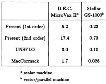
3.8 Euler Timing Study . . . . 85

4 Thin-Shear-Layer Navier-Stokes Algorithm 90 4.1 Objectives . . . . 90

4.2 Defect Formulation Revisited . . . . 91

4.4 Spatial Discretization . . . .

4.4.1 Cross-streamwise Discretization (ir-direction)

4.4.2 Streamwise Discretization (C-direction) . . . 4.4.3 Artificial Dissipation . . . .

4.5 Time Integration . . . .

4.5.1 Stability Analysis . . . .

4.6 Discrete Defect Equations . . . .

4.7 Boundary Conditions . . . .

4.7.1 Wall Boundary Conditions . . . . .

4.7.2 Edge Boundary Conditions . . . . .

4.7.3 Inlet/Exit Boundary Conditions . .

4.7.4 Leading Edge Boundary Conditions

4.8 Scaling Parameter . . . .

4.9 Cebeci-Smith Turbulence Model . . . .

4.10 Newton Solution Procedure . . . .

4.10.1 Newton's Method . . . .

4.10.2 Discrete Equation Linearization . . .

4.10.3 Jacobian Matrix . . . .

4.10.4 Gaussian Elimination . . . .

4.11 Similarity Profiles . . . .

4.11.1 Initial Profile Guess . . . .

4.12 Viscous Grid Generation . . . .

5 Euler/Navier-Stokes Coupling

5.1 Interpolation of Edge Solution . . . .

. 93 . 94 . 96 . 97 . 97 . 98 . 99 . 101 . 101 . 101 . 103 . 104 . 106 . 110 . 112 . 113 . 114 . 124 . 127 . 128 . 130 . 132 134 136 . . . .

5.2 Wall Transpiration Fluxes . . . . 137

5.2.1 Modification of Euler Wall Boundary Conditions . . . . 139

5.2.2 Numerical Integration of Mass Defect Equation . . . . 140

5.2.3 Proper vs. Approximate Transpiration Fluxes . . . . 141

5.3 Numerical Coupling Procedure . . . . 144

6 Discussion of Results 148 6.1 Results for Euler Algorithm . . . . 148

6.1.1 Subsonic Circular Bump . . . . 149

6.1.2 Transonic Circular Bump . . . . 151

6.1.3 Supersonic Circular Bump . . . . 152

6.1.4 Order of Accuracy Study . . . . 153

6.1.5 1-D Shock Tube . . . . 155

6.1.6 Unsteady Quasi-1-D Laval Nozzle . . . . 157

6.2 Results for TSL Navier-Stokes Algorithm . . . . 183

6.2.1 Blasius Similarity Solution . . . . 183

6.2.2 Turbulent Flat Plate . . . . 184

6.3 Results for Coupled Euler/Navier-Stokes Algorithm . . . . 192

6.3.1 Subsonic Compression Duct . . . . 192

6.3.2 Oblique Shock Impinging on a Laminar Boundary Layer . . . . . 193

6.3.3 Transonic Diffuser . . . . 197

7 Conclusions 226 7.1 Euler Algorithm . . . 226

7.3 Coupling Procedure . . . . 229

7.4 Recommendations for Future Research . . . . 231

7.4.1 Euler Recommendations . . . . 231

7.4.2 Navier-Stokes Recommendations . . . . 233

7.4.3 Coupling Recommendations . . . . 235

A Cell Metrics for Euler Algorithm 244 B Stability Analysis: Euler Algorithm 247 C Stability Analysis: TSL Navier-Stokes Algorithm 252 D Steady-State Acceleration 256 D.1 Euler Algorithm ... . 256

D.2 TSL Navier-Stokes Algorithm . . . . 261

E Test Case Descriptions 265

List of Figures

2.1 Control Volume . . . . 30

2.2 Laminar Boundary Layer on a Flat Plate . . . . 39

2.3 Inlet and Exit Farfield Boundaries for a Typical Geometry . . . . 47

3.1 Flux-Splitting for a Discontinuous Solution in 2-D . . . . 57

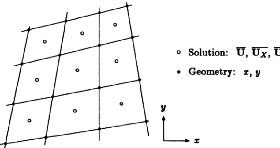
3.2 Euler Grid with Solution and Geometry Storage Locations . . . . 59

3.3 Constant Solution Approximation Within Cells (First Order) . . . . 59

3.4 Linear Solution Approximation Within Cells (Second Order) . . . . 61

3.5 Interpolation for Midpoint Rule Evaluation of Fluxes . . . . 61

3.6 Interpolation for Two-Point Gauss Quadrature of Fluxes . . . . 71

3.7 Effect of First-Stage Integration Constant on Stability Boundary . . . . 77

3.8 Numerical Entropy Rise Through a Stagnation Point . . . . 81

3.9 Normal Vectors for Actual Wall vs. Linear Wall Segment . . . . 85

3.10 Linear Wall Face Normals Used at Gauss Points . . . . 86

3.11 Analytic Wall Geometry Normals Used at Gauss Points . . . . 87

4.1 Viscous Grid Notation (computational space) . . . . 94

4.2 Laminar Separation Bubble in a Subsonic Expansion Duct . . . . 108

4.3 Predicted Edges of Viscous Grid Through Separation, (Eq. 4.33), Based on Fixed Grid Solution . . . . 109

4.4 Actual Edges of Viscous Grid Through Separation . . . . 109

4.6 Modified Block Jacobian Matrices at Boundaries . . . . 126

4.7 Block Jacobian Matrices for Global Equations . . . . 126

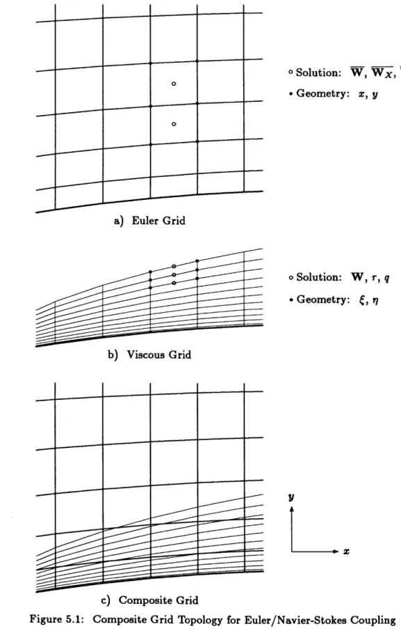
5.1 Composite Grid Topology for Euler/Navier-Stokes Coupling . . . . 135

5.2 Flow Chart for Numerical Coupling Procedure . . . . 145

6.1 Subsonic Circular Bump: M = 0.5, T = 10%, 64 x 16 grid, Character-istics Procedure . . . . 160

6.1 Subsonic Circular Bump: M = 0.5, r = 10%, 64 x 16 grid, Character-istics Procedure . . . . 161

6.2 Subsonic Circular Bump: M = 0.5, r = 10%, 64 x 16 grid, Velocity Reflection Procedure . . . . 162

6.3 Transonic Circular Bump: M = 0.675, r = 10%, 64 x 16 grid . . . . . 163

6.3 Transonic Circular Bump: M = 0.675, r = 10%, 64 x 16 grid . . . . . 164

6.4 Transonic Circular Bump: M = 0.675, r = 10%, 64 x 16 grid, Solution Interpolated to Nodes for Plotting . . . . 165

6.5 Supersonic Circular Bump: M = 1.4, r = 4%, 64 x 16 grid . . . . 166

6.5 Supersonic Circular Bump: M = 1.4, r = 4%, 64 x 16 grid . . . . 167

6.6 Order of Accuracy Study: Computational Grids . . . . 168

6.7 Order of Accuracy Study: Mach Number Distribution for 64 x 16 Grid 169 6.8 Order of Accuracy Study: Effect of Grid Resolution on Total Pressure Error ... ... ... ... .. ... ... ... ... ... . . .. . . 170

6.9 Order of Accuracy Study: Randomized Computational Grids . . . . . 171

6.10 Order of Accuracy Study: Mach Number Distribution for 64 x 16 Ran-domized Grid . . . . 172

6.11 Order of Accuracy Study: Effect of Grid Resolution on Total Pressure Error for Smooth and Randomized Grids . . . . 173

6.12 1-D Shock Tube Problem: Solution at t = 0.14492 . . . . 174

6.13 1-D Shock Tube Problem: Solution for Second Order Godunov Scheme

of Van Leer [831 . . . . 176

6.14 Laval Nozzle: Grid Comparison of Steady Pressure Distribution . . . . 177

6.15 Laval Nozzle: Unsteady Distribution of Pressure Due to a Sinusoidal Exit Pressure Oscillation of 15% Amplitude and Reduced Frequency of 2 178 6.16 Laval Nozzle: Grid Comparison of Unsteady Pressure Distribution Due to a Sinusoidal Exit Pressure Oscillation: Phase = 0 . . . . . 179

6.17 Laval Nozzle: Grid Comparison of Unsteady Pressure Distribution Due to a Sinusoidal Exit Pressure Oscillation: Phase = 90* . . . . 180

6.18 Laval Nozzle: Grid Comparison of Unsteady Pressure Distribution Due to a Sinusoidal Exit Pressure Oscillation: Phase = 1800 . . . . 181

6.19 Laval Nozzle: Grid Comparison of Unsteady Pressure Distribution Due to a Sinusoidal Exit Pressure Oscillation: Phase = 270* . . . . 182

6.20 Blasius Similarity Solution: Effect of Grid Refinement on Profiles . . . 186

6.21 Blasius Similarity Solution: Effect of Grid Refinement on Solution Error 187 6.22 Turbulent Flat Plate: Computational Grid, 30 x 48 . . . . 188

6.23 Turbulent Flat Plate: Skin Friction Distribution . . . . 189

6.24 Turbulent Flat Plate: Minimum Grid Spacing Along Plate . . . . 190

6.25 Turbulent Flat Plate: Velocity Profile at x = 4.08 . . . . 191

6.26 Oblique Shock/Boundary Layer: Experimental Geometry (from [8]) . . 194

6.27 Transonic Diffuser: Experimental Geometry (from [71]) . . . . 198

6.28 Compression Duct: Composite Grid and Flowfield . . . . 206

6.29 Compression Duct: Velocity Profiles Using TSL Navier-Stokes Equa-tions (Profiles at StaEqua-tions Indicated in Fig. 6.28a) . . . . 207

6.30 Compression Duct: Velocity Profiles Using Defect Equations (Profiles at Stations Indicated in Fig. 6.28a) . . . . 208

6.31 Oblique Shock/Boundary Layer: Coarse Computational Grid (Euler 64 x 16, Viscous 59 x 15) . . . . 209

6.32 Oblique Shock/Boundary Layer: Fine Computational Grid (Euler 128 x

32, Viscous 123 x 31) . . . . 210

6.33 Oblique Shock/Boundary Layer: Coarse Grid Density Contours (A = 0.005) . . . . 211 6.34 Oblique Shock/Boundary Layer: Fine Grid Density Contours (A = 0.005)212

6.35 Oblique Shock/Boundary Layer: Comparison of Separation Bubbles . 213 6.36 Oblique Shock/Boundary Layer: Comparison of Wall Pressure and Skin

Friction Distributions . . . . 214

6.37 Oblique Shock/Boundary Layer: Coarse Grid Density Contours (A = 0.005) for Unmodified Coupling Procedure . . . . 215

6.38 Oblique Shock/Boundary Layer: Coarse Grid Wall Pressure and Skin Friction Distributions for Unmodified Coupling Procedure . . . . 216

6.39 Transonic Diffuser: Grid and Mach Number Distribution for Entire Dom ain . . . . 217

6.40 Transonic Diffuser: Grid and Contour Plots for Diffuser Section . . . . 218 6.40 Transonic Diffuser: Grid and Contour Plots for Diffuser Section . . . . 219 6.41 Transonic Diffuser: Wall and Core Distributions for Diffuser Section . 220

6.41 Transonic Diffuser: Wall and Core Distributions for Diffuser Section . 221

6.42 Transonic Diffuser: Unsteady Static Pressure on Upper Wall at z/h* = 5.4222 6.43 Transonic Diffuser: Variation in Amplitude (rms) of Unsteady Static

Pressure Along Upper Wall . . . . 223

6.44 Transonic Diffuser: Solution of Defect Equations on Coarse Grid (Euler

48 x 8, Viscous 48 x 32) . . . . 224

6.45 Transonic Diffuser: Solution of TSL Navier-Stokes Equations on Coarse

Grid (Euler 48 x 8, Viscous 48 x 32) . . . . 225

7.1 Embedded Grid . . . . 232

D.1 Effect of Gradient Update Under-Relaxation on Stability Boundary of

List of Tables

3.1 Comparison of CPU Time (in psec) Per Cell Per Time Step ... 88

D.1 Effect of Relaxation and AF on Steady-State Convergence: Subsonic

Circular Bump on 32 x 8 Grid . . . . 261

D.2 Effect of Relaxation and AF on Steady-State Convergence: Transonic Circular Bump on 32 x 8 Grid . . . 262 D.3 Effect of AF on Steady-State Convergence: Turbulent Flate Plate With

Nomenclature

A, B, C,

G

F

F*

h

H

iJ

j

J*

A

q

R

R

S

t

U,

V

U, UX, UY

second area moments about cell centroid block Jacobian matrices

speed of sound

specific heats at constant volume, pressure skin friction coefficient

vector of characteristic variables static internal energy per unit mass total energy per unit mass

inviscid flux vector, see (2.3) split flux vectors, see (3.6) inviscid flux vector, see (2.3) static enthalpy per unit mass total enthalpy per unit mass inviscid flux vector, H = FI + Gj

computational coordinates (streamwise, normal to wall) Cartesian unit vectors

1-D Riemann invariants

coefficient of thermal conductivity

analytic operators (Euler, TSL Navier-Stokes, Defect) discrete operators (Euler, TSL Navier-Stokes, Defect) Mach number

unit vector normal to boundary or face static pressure

total pressure; Legendre polynomial Prandtl number

enthalpy flux

Cartesian heat transfer components velocity vector, q= ut + vj

perfect gas constant Reynolds number

viscous flux vector, see (2.4); vector of Newton residuals Euler residual vector (average, z and y-gradients) entropy, arclength from inlet

unit vector tangential to boundary or face Sutherland's constant, entropy

viscous flux vector, see (2.4) and (2.39) time

static temperature

Cartesian velocity components wall shear velocity

state vector of conservation variables

Euler conservation state vectors (average, z and y-gradients) Roe's parametric variables, see (2.74)

W W, WX, Wy z, y X

x)

IrXZ, 'my) ryy

state vector of Roe's parametric variables, see (2.74) Euler parametric state vectors (average, z and y-gradients) Cartesian position components

vector of Newton unknowns location of wall

ratio of specific heats, y = cp/c,, boundary layer thickness

boundary layer displacement thickness (incompressible) change or difference

time step size discrete error

vertical coordinate (computational space) Blasius' similarity variable

boundary layer momentum thickness (incompressible) Courant-Friedrichs-Lewy (CFL) number; characteristic diagonal matrix of characteristics A

coefficient of molecular viscosity coefficient of kinematic viscosity

smoothing coefficients in scaling parameter definition, see (4.37) streamwise coordinate (computational space)

static density

coefficient in scaling parameter definition, see (4.33) shear stress; time coordinate (computational space) components of shear stress tensor

frequency

control volume, boundary of control volume viscous grid scaling parameter

subscripts 0 C e energy extrap gi ghost J I, r 1, t m mass mom

inlet stagnation conditions cell centroid

edge of viscous grid; Euler parameter energy conservation equation

value extrapolated from computational domain interior Gauss points

value evaluated at ghost cell or point computational coordinate indices

edge of viscous grid (j = J)

left, right interpolated solution laminar, turbulent

face midpoint

mass conservation equation momentum conservation equation

n normal to boundary or face

ref reference conditions

8 tangential to boundary or face

t time derivative

spec value specified

v viscous parameter

w wall

x z-component or x-derivative

y y-component or y-derivative

upper, lower faces of viscous cell (j + 1, j)

superscripts

dimensional

( )

(

+ wall variable

left, right interpolated solution

h discrete quantity

(n) quantity at nth multi-stage level

Chapter 1

Introduction

Transonic flows at high Reynolds numbers are often dominated by the interaction of shocks with boundary layers. This interaction can also be naturally unsteady. Examples of such flows are engine inlets, where the shock and boundary layer in the diffuser section of the inlet can interreact with the compressor face in an oscillating manner. These oscillations are typically small but depending on geometries and flight conditions, they may become large, seriously degrading performance. Pressure oscillations of 20% magnitude have been observed experimentally [201.

Today prediction of 2-D unsteady, strongly interacting flowfields is becoming possi-ble with the tools of CFD. Because of the strength of the shock/boundary layer interac-tion and extent of viscous regions, these flowfields are presently simulated by algorithms solving the full Navier-Stokes equations everywhere. In principle, all relevant physics will be present in such solutions, but this is not necessarily the case. Within boundary lay-ers significant flow variations exist, which must be resolved to be accurately predicted. This requires local grid refinement, which in turn requires a priori knowledge of the boundary layer thickness--something that is part of the solution. Furthermore, these Navier-Stokes solvers typically use the same discretization throughout the flowfield. This has the advantage of simplicity in implementation, but it has several drawbacks. For example, viscous effects are calculated everywhere even though they are negligible throughout most of the flowfield. This results in wasted computing effort. Another drawback is that flowfields often include different features, such as shocks, boundary layers, acoustic waves, which are predicted by the same discretization. Each of these could be more efficiently solved by different algorithms.

the solution of strongly interacting flowfields, such as those involving unsteady shocks. The method developed in this thesis is a coupled 2-D Euler/Navier-Stokes algorithm. Separate but coupled algorithms are developed to solve the inviscid and viscous regions of the flowfield. Both the Euler and Navier-Stokes algorithms are designed to accurately predict the important physics of their respective regions.

The thesis consists of three major contributions: a new Euler algorithm for the outer inviscid flow, a new Thin-Shear-Layer Navier-Stokes algorithm for viscous regions, and a procedure for coupling the two together. Each of these three contributions are briefly described in the following sections.

1.1

Euler Algorithm

In the outer inviscid region, the 2-D Euler equations are used to model the flow since strong shocks and rotational flow may be present. Correct prediction of the Rankine-Hugoniot shock jump relations necessitates a conservative discretization. In addition it is desirable to capture moving shocks crisply, without pre- or post-shock numerical oscillations. There may also be low amplitude acoustic waves or weak shocks which physically propagate without being dissipated. In numerical calculations these may be dissipated or dispersed by excessive numerical errors, either in the form of truncation error or explicitly added artificial dissipation. Thus, it is important to minimize these errors.

Many Euler algorithms are in current use; most of these solve the unsteady Eu-ler equations in a time-marching manner, but were originally developed and tuned for steady calculations. Some of the more popular use central-differencing or partial up-winding, and may be separated into two classes: cell-centered and cell-vertex schemes.

Examples of the cell-centered algorithms include those of Pulliam and Steger [651;

and Jameson, Schmidt and Turkel [43]. These schemes have been formulated assuming a smooth, logically rectangular grid. They are spatially second order accurate on such

grids, but when used on nonsmooth (i.e. realistic) grids, their order of accuracy is re-duced, increasing numerical errors. In fact, Turkel [80 has analytically shown stringent restrictions on grid smoothness for achieving second order accuracy with a cell-centered central-differencing scheme in 1-D.

Cell-vertex algorithms include those of Ni [62]; Hall [38]; and Jameson [44]. In contrast to the cell-centered schemes, these cell-vertex schemes are second order accurate for steady-state regardless of grid smoothness [34]. For unsteady flows, grid assumptions reduce the spatial accuracy to first order for nonsmooth grids.

A feature of all these algorithms is that they must use explicitly added artificial dissipation or smoothing to capture shocks and constrain neutrally stable decoupled modes. Unfortunately, the added smoothing can reduce accuracy and robustness in several ways. First, the smoothing introduces user adjustable constants. Second, the smoothing to capture shocks is often different from that used to control decoupled modes. As a result, switches must be formulated to turn each on only where desired. Third, Lindquist [54,55] has shown for cell-vertex methods that care must be taken in constructing the smoothing operators to avoid reduced accuracy for nonsmooth grids. Furthermore, the smoothing operators need to be modified near boundaries; if poorly done, this can lead to divergence or nonphysical solutions [9]. Finally, the artificial dissipation is often constructed and tuned for steady-state. Because of this, numerical oscillations near shocks, that are small for steady-state, can become undesirably worse for unsteady flows.

Another class of algorithms gaining popularity are those that use flux-splitting, a form of upwinding. Members of this class include the schemes of Chakavarthy [19]; Bun-ing and Steger [14]; and Anderson, Thomas, and van Leer [7]. These methods attempt to use the underlying physics of the Euler equations more directly in their formulation. They have the advantage that they are often able to capture shocks without explicitly added artificial dissipation. They also do not allow decoupled modes. However, these schemes are cell-centered and suffer reduced accuracy on nonsmooth grids. In addition, they tend to be more dissipative than the central-differencing schemes on smooth grids.

This thesis presents a new algorithm for the solution of the 2-D unsteady Euler equations. The algorithm incorporates upwinding to capture shocks crisply and with minimal oscillations. To reduce numerical errors, grid independent second order accu-racy is achieved for both steady and unsteady flows. This is done by a formulation in which both averages and gradients are stored for each cell. The scheme allows no decoupled modes; hence, no explicitly added artificial dissipation is necessary. Thus, the present scheme retains many of the advantages of previous upwind methods without their poor accuracy on nonsmooth grids.

1.2

Thin-Shear-Layer Navier-Stokes Algorithm

In boundary layers, where viscous effects are important, the flow exhibits large vari-ations across the boundary layer (normal to the surface). Streamwise varivari-ations often remain comparatively small. As a result, the streamwise viscous stress gradients may be neglected and the region modeled by the Thin-Shear-Layer Navier-Stokes equations. An exception to this situation is when shocks impinge on the boundary layer. Then streamwise flow variations are large, with near step discontinuities in the outer part of the boundary layer and complex compression structures lower in the boundary layer. If macroscopic changes are desired, rather than these fine structures, then the streamwise viscous stress gradients may still be neglected as long as the equations are solved in a conservative formulation.

The large flow variations across the boundary layer place special requirements on numerical algorithms. To best predict these variations, high accuracy is important for the discretization normal to the surface. This is true not only for inviscid terms but also for viscous terms. In addition, resolution of these large variations can result in very small grid spacing normal to the surface, especially for turbulent cases. Schemes using explicit time integration are limited by numerical stability to a time step proportional to this small spacing. Thus, the choice of time integration becomes important. Finally, the thickness of the boundary layer itself becomes a numerical problem. Although a part of the solution, it must be known to specify an appropriate grid. Accurate

knowledge of the thickness cannot be known a priori in many flows, such as those involving shock/boundary layer interaction or large separation.

Typically, Navier-Stokes algorithms are developed from existing Euler algorithms by adding discretized viscous terms. Examples are the schemes of Beam and Warm-ing [10]; Swanson and Turkel [78]; Rai [66]; Davis, Ni, and Bowley [26]; and Thomas and Walters [79]. In all of these schemes, the viscous stresses are discretized by 3-point central-differencing assuming a uniform grid. For the highly stretched grids (i.e. large cell size variation) used for viscous simulations, these fail to be second order accurate. Those schemes that do not use flux-splitting for the inviscid terms [10,26,78 require artificial dissipation to damp decoupled modes. Construction of these operators is par-ticularly crucial for viscous regions since they can contaminate solutions by masking physical viscosity [2,26}.

An extension of the Euler algorithm presented in this thesis to Navier-Stokes would suffer from some of these same disadvantages. Even with the solution averages and gra-dients stored for each cell, unconditional second order accuracy for the viscous stresses would not be possible. Furthermore, the scheme uses explicit time integration. For these reasons, this thesis also presents a separate TSL Navier-Stokes algorithm designed to meet the requirements of viscous regions.

The main objectives of this development have been second order accuracy for both inviscid and viscous terms across the boundary layer, a time integration which uses practical time steps, and a means of adapting the grid to the changing boundary layer thickness. The first objective is met by a discretization across the boundary layer which is similar to that used in the Keller Box scheme [48] for the solution of the Boundary Layer equations. It is second order accurate for both inviscid and viscous terms on highly stretched grids. To capture shocks in the outer flow, upwind differencing is used in the streamwise discretization. The resulting spatial discretization has no unconstrained decoupled modes and needs no added artificial dissipation.

To meet the second objective, the algorithm incorporates a semi-implicit time in-tegration. Discretization normal to the surface is integrated implicitly and that in the

streamwise direction is integrated explicitly. Hence, the solution can be integrated at a time step depending on the streamwise grid spacing only. For a given streamwise station and time step, the implicit system is solved by Newton's method.

The third objective is realized by a dynamic coordinate transformation. The coordi-nate normal to the wall is rescaled by the unsteady local boundary layer thickness, and the transformed equations solved on a fixed grid. A similar adaptive procedure has been used by Carter [16] and Drela [28] for the solution of the Boundary Layer equations.

1.3

Viscous/Inviscid Coupling

Separation of the flow into viscous and inviscid regions requires coupling or commu-nication between the different regions to properly solve the entire flowfield. Hence, the third and final major contribution of this thesis is a procedure for coupling the Euler and TSL Navier-Stokes algorithms together.

Previous methods for viscous/inviscid coupling using the Euler and Navier-Stokes equations have been zonal approaches. The viscous and inviscid regions are separated from one another and coupling is through information transfer near the interface. Two variants of the zonal approach exist: patched grids and slightly overlapping grids.

In patched grid approaches, such as Rai [66,67] and Nakahashi [61], a Navier-Stokes grid is constructed about the body to a predetermined point, and then an Euler grid constructed abutting it. Coupling between the grids is by conservative evaluation of the fluxes along the interface. A drawback of this approach is placement of the interface. If the interface is fixed, then it must be placed well outside viscous regions. However, this requires a priori knowledge of boundary layer thicknesses. On the other hand, if the interface is allowed to move, then the entire domain must be regridded.

In overlapping grid techniques, such as Denek et al [27], coupling between the dif-ferent grids is through solution interpolation in the overlap region. This requires both solutions to be physically realistic in the region of overlap. Hence, for

Euler/Navier-Stokes coupling the entire overlap must be well outside any viscous regions. In this approach a conservative formulation near the interface is very difficult. A further com-ment is that flowfields calculated by Rai [66] using both patched and overlapping grids show noticeable numerical noise in overlap regions, and Rai seems to have abandoned using overlapping grids in favor of patched grids for similar test cases in later papers.

In all the references listed above, the same inviscid discretization has been used in each region. If different algorithms are used in each region and the solution matched at the interface, then differing truncation errors will cause a numerical boundary layer in the vicinity of the interface. Therefore, special treatment (such as smoothing) near the interface would be required to avoid these nonphysical boundary layers.

For these reasons, an alternative form of coupling is used this thesis. The flowfield is solved on overlapping grids with the Euler grid extending to the body surface. That portion of the Euler solution within the viscous region is computed but is not physi-cally meaningful. Coupling between the Euler and Navier-Stokes solutions is through boundary conditions-specified outer edge values for the viscous solution and wall tran-spiration fluxes for the Euler solution. Coupled in this manner, the Euler grid remains fixed while the viscous grid evolves with the changing boundary layer thickness. Thus, a priori knowledge of boundary layer thicknesses is not required to solve the flow accu-rately.

This form of coupling is closer to viscous/inviscid interaction techniques solving the Boundary Layer equations within viscous regions. Examples of algorithms using the Potential equations for the inviscid flow are those of Le Balleur [49,50,51] and Carter [17]. Algorithms modeling the inviscid flow by the Euler equations have been developed by Johnston and Sockol [45]; Whitfield et al [88]; Bussing and Murman [15,60]; Savant and

Wigton [72]; and Drela and Giles [30].

These coupling methods are based on different but equivalent viewpoints of the boundary layer's effect on the outer inviscid flow. Lighthill [53] has shown that the primary effect of the boundary layer is a displacement of the inviscid streamlines away from the surface of the body. For the solution of the outer inviscid flow, this effect can

be produced by physically enlarging the body by the local displacement thickness of the boundary layer. Thus, one coupling method is to construct an inviscid grid outside the displacement surface, where a zero normal mass flux condition is specified. This method was used by Drela and Giles [30], where the grid was solved as part of the solution. For use with a conventional Euler or Potential solver, this coupling method has the disadvantage that the grid must be regenerated as the displacement surface changes.

Lighthill also showed that the displacement effect can equivalently be produced by a distribution of sources along the surface of the body; this results in transpiration or blowing at the surface. Thus, the inviscid flow is solved to the body surface, where transpiration fluxes are specified; these are obtained from an integration of the viscous equations across the boundary layer. An advantage of this method is that the inviscid grid is fixed and need be generated only once. This coupling method was used by all others listed. It is also the method of choice in this thesis. Thus, this thesis repre-sents the first extension of coupling through transpiration fluxes to the solution of the

Euler/Navier-Stokes equations.

A feature of the present coupling is the use of the Defect formulation of Le Balleur [50,51]. An important aspect of this approach is the solution of the TSL Navier-Stokes equa-tions written in the form of Defect equaequa-tions within viscous regions. With different algorithms solving the inviscid and viscous equations, the discrete Defect equations subtract off the relative truncation error. This allows the inviscid and viscous solutions to match smoothly at the edge of the viscous grid. In principle, it also makes a con-servative formulation at the interface possible; in this it has a potential advantage over other overlapping grid techniques.

1.4

Overview of Thesis

Chapter 2 presents the governing equations for fluid motion, including nondimen-sionalization and an asymptotic analysis to simplify them for the flowfields of present

interest. The resulting equation sets are the Euler and Thin-Shear-Layer Navier-Stokes equations. Boundary conditions and a parametric state vector used in both the Euler and Navier-Stokes algorithms are also discussed.

The development of the Euler algorithm is presented in Chapter 3. A first order upwind scheme, similar to existing methods, is first discussed. It is then extended to second order accuracy by a new approach of using both cell averages and gradients. An explicit time integration is then presented, along with a stability analysis for both the first and second order discretizations.

Chapter 4 develops the TSL Navier-Stokes algorithm. A dynamic coordinate trans-formation is defined. Then the different streamwise and cross-stream spatial discretiza-tions are developed. This is followed by the semi-implicit integration for evolving the viscous solution in time. Minor modifications of the discrete equations are then discussed for implementing the Defect formulation. This chapter concludes with a discussion of the Newton solution procedure for the implicit system resulting from the semi-implicit time integration; it includes equation linearization and direct solution of the linearized system by Gaussian elimination.

Chapter 5 describes the procedure used to couple the Euler and Navier-Stokes al-gorithms together. This includes interpolation of the Euler solution for edge boundary conditions on the viscous solution, and integration of the viscous equations across the boundary layer for wall transpiration fluxes. This chapter concludes with a flowchart of the numerical coupling procedure.

Chapter 6 presents a series of numerical test cases to demonstrate the capabilities of the Euler algorithm, the TSL Navier-Stokes algorithm, and the coupling procedure. Two-dimensional channel flow test cases for Euler solvers are first presented. Then an order of accuracy study is conducted to numerically demonstrate the second order accuracy of the Euler algorithm on smooth and randomized grids. Its unsteady shock tracking capabilities are demonstrated for two test cases. The first is a 1-D shock tube problem, where results are compared to the analytic solution; and the second is a quasi-1-D Laval nozzle, where it is compared to the central-differencing scheme of Jameson.

The second order spatial accuracy of the cross-stream discretization in the TSL algorithm is verified using Blausius' similarity solution for laminar flat plate flow. This is followed by a turbulent flat plate case verifying the correct implementation of the turbulence model; results are compared with experiment.

The fully coupled Euler/Navier-Stokes algorithm is then demonstrated for both steady and unsteady flows using three test cases. The first test case is a laminar boundary layer in a subsonic compression duct. It is used to demonstrate the nu-merical improvements resulting from the solution of the Defect equations. The second is a steady oblique shock impinging on a flat plate laminar boundary layer. Surface pressure and friction coefficients are compared with experiment. The third and final test case is a transonic diffuser with turbulent boundary layers. The algorithm is used to detect self-induced unsteadiness in the shock/boundary layer interaction found in experiments.

Chapter 2

Governing Equations

The equations governing the motion of a fluid are presented in this chapter. No at-tempt is made to derive the equations; detailed derivations can be found elsewhere [87,73,52,6]. Instead the governing equations will be stated briefly along with major assumptions made. Subsequent analysis, including nondimensionalization and asymptotic analysis to simplify the governing equations, will be presented in more detail since they are more pertinent to material covered in this thesis. This chapter will conclude with additional analysis of inviscid characteristics for boundary conditions and representation of the inviscid conservation and flux vectors by a parametric vector.

2.1

2-D Navier-Stokes Equations

The motion of a compressible, two-dimensional (2-D) fluid is governed by the Navier-Stokes equations. These represent the conservation of mass, momentum and energy in a fixed control volume, such as that shown in Figure 2.1. In differential form the equations are given by,

mass:

+

aP

+

Pv

0

_at

_ax

_a

1

y

x-momentum:

apu+ 8pu

+

+pt a

a

+

at

ax

a

y

ax

ax

ay

8pv apuv apv2

ap

y-momentum:

+

+

a+

-

a

+

ai

at ax a y ay ax ay

apE apuH apvH

a

energy:at + a +

a

qz

+

+

a-

(qy

+

(2.1a)

(2.1b)

(2.1c)

na

Figure 2.1: Control Volume

In these equations p is density, p is pressure, E is total internal energy, H is total enthalpy, and uf + vi is the velocity vector (u and v are the Cartesian components in the x and y directions, respectively). Viscous effects are represented by the shear stress tensor (7',,, ry, Ty1) and the heat conduction vector qgS + qyj.

The governing equations may also be written in a more convenient vector form,

aU aF aG 8R

aS

+ -

+ --

a+(2.2)

a

x &

ay y

where the conservation vector U and inviscid flux vectors F and G are defined as,

P Pu

(

U

(P

F =

(2.3)

PVPut

jpt)

_{+ p}

pE k puH

I

and R and S contain the viscous terms,

0 0

R =

,

S =I.

(2.4)

-qz+ uriz+vrzy

-qp+u-rx+v

ry)

The Navier-Stokes equations may also be written in integral form,

where the integral is over the control volume fl bounded by the curve 8; n^ is the unit outward normal to fl. The integral and differential forms are equivalent for continuous solutions; one is obtained from the other by the divergence theorem. The integral form is more general, since it is valid for discontinuous solutions. It will be used as the starting point for the finite volume algorithm of Chapter 3. The differential form will be used for further analysis and the starting point for the finite difference algorithm of Chapter 4.

In writing the Navier-Stokes equations, several assumptions have been made. The first is that the density is high enough that the fluid may be approximated as a contin-uum rather than discrete molecules. Other assumptions are that no chemical reactions, mass diffusion, or heat addition through radiation occur. Inclusion of these effects re-quires major modifications to the numerical algorithms presented in this thesis. A fur-ther assumption is the absence of body forces, including gravity, electromagnetic forces, three-dimensional rotation effects, etc. Typically, body forces appear in the equations as source terms (undifferentiated), which are easily modeled. Thus, modification of the present theory to include these effects is minor.

Apart from these assumptions, Equations (2.1) are quite general, since the viscous stresses and heat transfer have been left undefined. To solve the equations, these need to be specified. In addition, an equation of state relating the thermodynamic variables (p, p, E and H) is required.

The fluid is assumed to be a Newtonian fluid in which the shear stresses are linearly dependent on the fluid strain rates; it is also assumed to satisfy Stokes' hypothesis. With these assumptions, the components of the stress tensor may be written as,

c') 2 au av 2 au a V

rc = 21s- -1A

-

+

,r,, =

ay

a +

Y

a

(2.6b)

09U

av

(--Y

+

-),

(2.6c)

where p is the coefficient of molecular viscosity. Consistent with a Newtonian fluid is Fourier's law, which states that the heat transfer is linearly dependent on temperature

gradients,

qz = -k-T q, = -k---, (2.7)

5 - ay

where T is temperature and k is the coefficient of thermal conductivity.

The set of equations is closed by an equation of state relating the thermodynamic variables, as well as relations for yu and k. Here a perfect gas is assumed,

p = pRT, R = gas constant. (2.8)

Assuming further that the gas is calorically perfect (i.e. the specific heats c, and c,, are constant), then the static and total internal energy are given by,

e = cT, E = e + 1(u2 + v2), (2.9)

and the static and total enthalpy by,

h = cPT, H = h+ (u2 +v 2). (2.10)

Further useful relations are,

pH = pE + p, (2.11)

p = (y -1) PE - 1p(u2 + V2)], (2.12)

P i pH - p(s2 + V2)], (2.13)

l 1 2 1

where y = cp/c, is the ratio of specific heats (-y = 1.40 for air) and R = c, - c,.

For a perfect gas the coefficients of molecular viscosity and thermal conductivity are functions only of the temperature. Sutherland's law for the molecular viscosity is employed,

y _{-- = (-32}

(

(2.14)

Aref Tref T+S '

where S is Sutherland's constant (S = 110K for air), Tref is some reference temperature and pref is the molecular viscosity measured at that temperature. For air Sutherland's law is accurate to within 2% over a wide range of temperatures [87, p 28-29]. For most gases the thermal conductivity is approximately proportional to the molecular viscosity. Here this relation is assumed exact,

k = A(2.15)

2.1.1 Boundary Conditions

Boundary conditions are necessary to define a unique solution. For the physical problems presented in this thesis, conditions at two different types of boundaries need be considered. The first are solid wall boundaries. Because of friction, fluid in contact with a wall must not move relative to the wall; this is the no-slip condition. For a stationary wall this gives,

at wall: u=0, v=0. (2.16a)

Only stationary walls are considered in this thesis. In addition, the fluid in contact with the wall must have the same temperature as the wall or the same heat transfer as the wall,

at wall: T = Tw or (q + qyj) - h = qw. (2.16b)

Only adiabatic walls (qw = 0) are considered in this thesis.

The second type of "boundary" is the flow far from the wall or body, where the flow approaches some known uniform or stagnation conditions. The treatment of these farfield boundary conditions for numerical computations is presented in Section 2.4.

2.1.2 Nondimensionalization

Nondimensionalization is performed on the Navier-Stokes equations before they are analyzed. From this process, certain nondimensional groups emerge whose magnitudes can be used to characterize the behavior of solutions.

In the following, dimensional quantities are denoted with a bar

( ),

heat constant ZPref:

X= i y=

t=-Lref Lre' Lref/Cref

Pu U

Pref Cref Cref (2.17)

pEH

P= , E= - H - 2 >

Pref Cref Cref cre

___ k

T= p= k= .

Cref/CPref Aref kref

The shear stresses

(

= q = - . (2.18)

Areferef /Lref' Arefrefflref

In addition, the nondimensional specific heats and gas constant become,

__ ce 1 R _ '-l

c,=_ =1, cV-._ -

,

CPref CPref 'CPref y

When these definitions are substituted into the Navier-Stokes equations (2.1), two nondimensional parameters emerge. The first is the Reynolds number,

Re = prefiref Lref (2.20)

Pref

which results from comparison of the groups used to nondimensionalize inviscid and viscous terms in each equation. The second is the Prandtl number,

Pr = PrefCPref (2.21)

kref

which results from comparison of the definition of the heat transfer (2.7) and the group used to nondimensionalize it.

The resulting nondimensional Navier-Stokes equations are modified from (2.1) only by a factor of 1/Re multiplying the viscous terms,

aU

aG

aS

---

+

_axo

_aiy

The nondimensional vectors U, F, G, R and S are unchanged from (2.3) and (2.4). With the exception of the heat transfer definition (2.7) and Sutherland's law (2.14), the rest of the equations previously listed retain their forms when nondimensionalized. The nondimensional heat transfer definition is modified by the presence of the Prandtl number, _ -8_ k OT q.=-k- =& q= ---- , (2.23a) ay Pr

az

a

k--.

ay

ay

It will be more convenient to write the heat transfer in terms of p and H instead of k and T. Thus, using (2.10),

qz = ---

[--

u

Pr

( ;

ax]

qy = - - --- -u - . (2.24b)

Pr pcP

5-y -

y UY_

y

From (2.15) and (2.19), the group k/psc is unity and will be dropped from this point forward.

Sutherland's law (2.14) poses a problem due to the presence of 9, which becomes a user input in nondimensional form along with the Reynolds and Prandtl numbers. If nondimensionalized by the group ir2f/Zref, it becomes awkward to compute. Thus, in this equation T and 9 are chosen to be nondimensionalized by the reference temperature

Tref,

A ='= _ , '(2.25)

Aref Tref Tref

where the prime indicates a different nondimensionalization from that used in the gov-erning equations. Substitution into Sutherland's law gives,

yA T'/

(2.26) pAref Tref T'O+ S'

where pref = 1 and Tr'ef = 1. The relation of Tref _{and T' to the rest of the variables is by} the choice of reference conditions. In this thesis, inlet plenum or stagnation conditions

are used, where eref is the stagnation speed of sound,

Pref = O, Cref = o, Tref = ,

(2.27)

The speed of sound is given by,

=C = . (2.28)

Therefore, using the perfect gas relation the reference temperature becomes, -21 -2

Tref = Ce = Iref (2.29)

,yR Y - 12 Eref

and the nondimensional temperature becomes,

h

T'= (-y - 1)T = (-I - 1). (2.30)

cp

2.1.3 Turbulence Modeling

The Navier-Stokes equations in their present form admit turbulent behavior for high Reynolds number flows. Turbulence is unsteady stochastic flow characterized by a wide range of length scales, and resolution of all these scales for practical geometries is be-yond present day computing resources. To make the problem of turbulence manageable, the governing equations are statistically averaged, and mean rather than instantaneous quantities solved for. The resulting equation set is known as the Reynolds averaged (or more precisely, mass or Favre averaged for compressible flows) Navier-Stokes equations. They are modified from the original equations by apparent stresses, resulting from the averaging of nonlinear terms, which must be modeled through empirical correlations. Here the Boussinesq approximation is used; these apparent stresses are assumed pro-portional to the mean strain rates and temperature gradients, similar to the molecular viscosity (2.6) and heat transfer (2.7). The essence of the approximation is a redefinition of A and k,

A = JI + Pt, k = k, + kt, (2.31)

where pj and k are the laminar or molecular viscosity and heat conduction coefficients used previously, and At and kt are their turbulent counterparts. The turbulent Prandtl number,

Prt = AtpCP (2.32)

is assumed constant; the value Prt = 0.9 is used here. The resulting Reynolds averaged shear stress tensor and heat conduction are given by,

2

1

gy )'

(

p_

[

8H

au

av1

=

_*

_P

_Pr

-

v

].

oy

ay

ay

In future equations if the

( )

2.2

Asymptotic Analysis

Aerodynamic problems are often characterized by high Reynolds numbers (Re 106). Hence, they may be mathematically classified as singular perturbation problems, because the highest order derivatives are multiplied by a small parameter. Solutions

exhibit "boundary layer" behavior where the importance of the viscous terms (highest

order derivatives) is confined to thin regions near boundaries. Within these layers the viscous terms become the same order as the inviscid convection terms, and the solution gradients become large. Outside these layers, viscous effects are negligible, and solution gradients are fairly small. Furthermore, certain viscous terms typically dominate over others within these boundary layers.

Since this discovery by Prandtl in 1904, a great deal of research effort has been

expended deriving and solving simplified versions of the Navier-Stokes equations. In this section some of this analysis is repeated to derive simplified equation sets.

2.2.1 Euler Equations

Consider the flow outside of the boundary layers. The solution gradients are small, thus the viscous stresses are negligible compared to the inviscid terms. Formally, this can be analyzed by taking the limit of Re -+ oo. The resulting equations are known as the Euler equations:

aU

at

ax

ay

(

U

=

P

F

=

(2.34c)

This is a system of first order equations, whereas the full Navier-Stokes equations are a system of second order equations. A consequence of this is loss of boundary conditions, in particular the no-slip and heat transfer constraints at a wall. Only the boundary condition of no mass flux through the wall may be retained,

Solid wall: (us + VJ) A = 0, (2.35)

where n is the normal to the wall; this is also referred to as a slip condition. Neglecting shear stress and heat transfer, boundary conditions far from the body (i.e freestream conditions) are unchanged from the full Navier-Stokes equations. They are treated in detail in Section 2.4.

2.2.2 Thin-Shear-Layer Navier-Stokes Equations

For many geometries, properties within a boundary layer are changing slowly in the streamwise direction even though variations normal to the wall are large. Thus, viscous stresses normal to the wall dominate those in the streamwise direction. This