HAL Id: hal-02117662
https://hal.archives-ouvertes.fr/hal-02117662
Submitted on 2 May 2019
HAL is a multi-disciplinary open access
archive for the deposit and dissemination of
sci-entific research documents, whether they are
pub-lished or not. The documents may come from
teaching and research institutions in France or
abroad, or from public or private research centers.
L’archive ouverte pluridisciplinaire HAL, est
destinée au dépôt et à la diffusion de documents
scientifiques de niveau recherche, publiés ou non,
émanant des établissements d’enseignement et de
recherche français ou étrangers, des laboratoires
publics ou privés.
Memory effects in a random walk description of protein
structure ensembles
Gerald R. Kneller, Konrad Hinsen
To cite this version:
Gerald R. Kneller, Konrad Hinsen. Memory effects in a random walk description of protein structure
ensembles. Journal of Chemical Physics, American Institute of Physics, 2019, 150 (6), pp.064911.
�10.1063/1.5054887�. �hal-02117662�
1Centre de Biophys. Mol´eculaire, CNRS; Rue Charles Sadron, 45071 Orl´eans, France 2
Universit´e d’Orl´eans; Chateau de la Source-Av. du Parc Floral, 45067 Orl´eans, France and
3
Synchrotron Soleil; L’Orme de Merisiers, 91192 Gif-sur-Yvette, France
In this paper we show that ensembles of well-structured and unstructured proteins can be dis-tinguished by borrowing concepts from non-equilibrium statistical mechanics. For this purpose, we represent proteins by two different polymer models and interpret the resulting polymer configura-tions as random walks of a diffusing particle in space. The first model is the trace of the Cα-atoms
along the protein main chain and the second their projections onto the protein axis. The resulting trajectories are subsequently analyzed using the theory of the Generalized Langevin Equation. Ve-locities are replaced by displacements relating consecutive points on the discrete protein axes and equilibrium ensemble averages by averages over appropriate protein structure ensembles. The re-sulting displacement autocorrelation functions resemble those of velocity autocorrelation functions of simple liquids and display a minimum, which can be related to the lengths of secondary structure elements. This minimum is clearly more pronounced for well-structured proteins than for unstruc-tured ones and the corresponding memory function displays a slower decay, indicating a stronger “folding memory”.
PACS numbers: Keywords:
I. INTRODUCTION
The protein structure-function relationship is one of the basic concepts in structural biology and it has for several decades driven the determination of protein struc-tures by X-ray and neutron crystallography as well as by nuclear magnetic resonance (NMR) techniques. It was soon recognised that protein function requires dy-namic structures,1–4 and one can observe a change in
paradigm over the last years, admitting that protein function does not necessarily require well-defined struc-tures. One speaks here of intrinsically disordered pro-teins (IDP), where the term “disorder” describes the ab-sence of well-defined secondary structure elements and may concern the whole protein or parts of it.5–8 In con-trast to well-structured proteins, for which more than 140000 structures can be found at present in the Pro-tein Data Bank9, much less is known about the possible
conformations of IDPs. Information comes here essen-tially from computer-generated models which are com-patible with experimental data from structural NMR and small angle diffraction techniques. Corresponding data bases are being built up10,11 and start to become
ex-ploitable from a statistical point of view. One can there-fore search for criteria that allow a distinction between structured and unstructured proteins on a purely statis-tical basis. Since protein structure data bases contain structures and structure ensembles of different proteins, such statistical models should be based on the confor-mation of the protein main chain only. The simplest ex-ample is the polymer chain model by W. Kuhn,12 which
consists of equidistantly spaced point-like monomers and which can be transposed to proteins by associating each Cα-atom along the protein main chain with a monomer
of the Kuhn chain. We note here that that due to the
rigid geometry of peptide bonds, the distances between consecutive Cα-atoms in proteins have an almost
con-stant value of 0.4 nm. The polymer configurations in Kuhn’s model are random chains, where all monomers are placed randomly at the fixed distance to their respec-tive predecessor along the polymer chain. These freely jointed chains lead to a Gaussian model for the prob-ability distribution of finding a monomer at a distance r from a given monomer and they can be interpreted as trajectories of Brownian particles whose subsequent posi-tions in time correspond to the monomer posiposi-tions along the polymer chain. The Markovian character of Brow-nian motion reflects the fact that the position of each monomer depends only on the position of its predecessor. The Gaussian chains thus have “zero folding memory”. Kuhn’s model was the motivation for the present work, where the concept of folding memory will be used in or-der to distinguish between ensembles of well-structured and (partially) unstructured proteins (IDPs).
II. PROTEINS AS DISCRETE PATHS In the standard discrete path representation of pro-teins, each residue is represented by its Cα-atom. In the
following, we will both this standard representation and an alternative one, in which secondary structure elements (SSEs) are essentially filtered out. SSEs are characterised by a regular winding of the protein main chain with a typical period between 2 and 4 monomers (residues) and thus lead to a priori “trivial” folding memory ef-fects on that scale. Our straightened path representa-tion replaces SSEs by the axis around which the main chain is wound. This axis can be obtained using the ScrewFrame algorithm.13 The global fold of a protein is
2
FIG. 1: Left: Exact helicoidal trace of Cα-atoms (red points)
and corresponding screw motion centres (blue points). The figure also shows two consecutive Frenet frames (black ar-rows), which are attached to Cα-atoms 2 and 3, respectively.
Right: Cα-trace and corresponding screw motion centres for
myoglobin (PDB structure code 1AB6). The local radius of the gray tube is defined by the radius of the corresponding screw motion.
described as a succession of screw motions aligning suc-cessive discrete Frenet frames along the Cα-trace. The
centres for the constructed screw motions then define a “polymer chain” along the protein axis. In contrast to the Cα-trace, where the distances between adjacent Cα
-atoms are nearly constant, ∆ ≈ 0.38 nm, the distances between adjacent screw motion centres vary and are con-siderably shorter. The protein axis polymer chain may be associated with a Rouse chain, where the monomers are connected by springs.14
The left part of Fig. 1 illustrates the construction of the screw motion centres (blue points) from a Cα-trace (red
points) which has the form of an ideal helix, such that the corresponding screw motion centres lie on a straight axis (except for the first and the last one). The two Frenet frames shown in black define the screw motion from “monomer” 2 to 3. For N Cα-atoms there are N −1
screw motion centres. The right part of the figure shows the corresponding analysis for myoglobin (PDB structure code 1AB6). It is important to note that ScrewFrame is applicable to any Cα-trace, i.e. also to β-strands, which
are “flat helices”, and for unstructured parts of a pro-tein. Secondary structure elements are characterised by recurrent screw motion parameters and in particular by a straight axis joining the screw motion centres. The ScrewFrame algorithm leads effectively to a tube model for proteins (indicated in transparent grey), where the local tube axis is defined by the succession of screw mo-tions centres and the local radius by the radius of the respective screw motion. The tube can be considered as excluded volume of the protein main chain. In polymer physics, tube models are used to explain the slow dynam-ics of reptation,15,16 where the tube represents the space
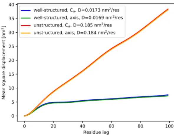
accessible to a single polymer inside the polymer matrix forming its environment, but the reptation model is ob-viously not a valid picture for the dynamics of protein main chains. 0 20 40 60 80 100 Residue lag 0 5 10 15 20 25 30 35 40 Me an sq ua re d isp lac em en t [ nm 2] well-structured, C , D=0.0173 nm2/res
well-structured, axis, D=0.0169 nm2/res
unstructured, C , D=0.185 nm2/res
unstructured, axis, D=0.184 nm2/res
FIG. 2: Mean square displacement as a function of residue lag for well-structured and unstructured proteins. In both cases the MSDs are shown for the Cα-traces and for the protein
axes.
III. DIFFUSIVITY OF PROTEIN PATHS A. Mean square displacements
Starting from the analogy between polymer mod-els and discrete stochastic paths, we consider first the ensemble-averaged mean square displacement (MSD)
W (n) = * 1 Nx− n Nx−1−n X k=0 (x(k + n) − x(k))2 + , (1)
where Nx is the number of steps in the discrete path,
x(k) (k = 0, . . . , Nx − 1), and n = 0, . . . , P Nx
to obtain good statistics. For our calculations we used P = 100. The brackets in (1) denote an average over the protein structures in the given ensemble, where each protein structure counts equally. This weighting scheme, which corresponds to unconstrained maximum entropy weighting17, is very different from thermal averaging of
configurations in statistical mechanics, where each con-figuration is weighted with a Boltzmann factor. Eq. (1) is constructed in complete analogy with time-dependent MSDs, as they are for example calculated from single particle tracking in biological systems or from molecular dynamics simulations. MSDs of discretely sampled tra-jectories are traced as a function of the time lag n ≡ n∆t, where ∆t is the sampling step, whereas the MSDs pre-sented in this paper are traced as function of the dimen-sionsless “residue lag”. In this context, it may appear more appropriate to speak of “mean square distances” instead of “mean square displacements”, because we are not considering moving particles. However, we keep the first term in order to maintain the analogy with trajec-tory analyses.
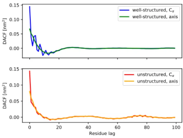
0.00 0.05 0.10 0.15 DA CF [n m 2] well-structured, C well-structured, axis 0 20 40 60 80 100 Residue lag 0.00 0.05 0.10 0.15 DA CF [n m 2] unstructured, C unstructured, axis
FIG. 3: Upper panel: DACFs for well structured proteins comparing the Cα-traces and protein axes. Lower panel:The
same for unstructured proteins.
Fig. 2 shows the MSD as a function of residue lag for well-structured and unstructured proteins. In the first case we used protein structures from the ASTRAL data base18,19 and in the second from the pE-DB data base.10
The diffusion coefficients indicated in the plot have been obtained by fitting a linear expression of the form
W (n) = 2Dn + a (2) to the MSD data for n ≥ 20. This offset appears clearly in the data for well-structured proteins and corresponds roughly to the maximum length of protein secondary structure elements. Practically no differences can be found between the MSDs for the Cα-trace and the protein
axis, but the diffusion coefficient for unstructured pro-teins is about ten times larger than for well-structured proteins. We find D ≈ 0.18 nm2/res. in the first case
and D ≈ 0.017 nm2/res. in the second. Using the the
polymer-trajectory analogy, the asymptotic linear form of W (n) for both well-structured and unstructured pro-teins corresponds to “normal diffusion”. From this point of view they behave like Gaussian chains or, equivalently, like trajectories of Brownian particles. As we will show in the following, the local behaviour is, however, very different.
B. Displacement autocorrelation functions In order to investigate the local properties of our two polymer models for well-structured and unstructured proteins, we make use of a well-known relation between the time-dependent MSD for a diffusing classical par-ticle and its velocity autocorrelation function (VACF), cvv(τ ) = hv(0) · v(τ )i. Assuming stationarity of the
W (t) = 2 Z t
0
dτ (t − τ )cvv(τ ), (3)
were h. . .i denotes a classical ensemble average over the phase space of the diffusing particle. The VACF itself fulfils an equation of motion of the form21
˙cvv(t) +
Z t
0
dτ κv(t − τ )cvv(τ ) = 0, (4)
where the memory kernel κ(t)vcan be formally expressed
by the microscopic forces acting on the diffusing parti-cle and between the solvent partiparti-cles. In the following, only use the general form of the equation of motion (4) is of importance. At the velocity level, the motion of a Brownian particle is described by the Langevin equa-tion, ˙v(t) + γv(t) = fs(t), where fs(t) is white noise,
γ > 0 a friction constant. The memory kernel has the form κv(t) = γδ(t), where δ(t) is the Dirac delta
func-tion. Brownian motion is thus “memory-less” and the VACF has the form cvv(t) = h|v|2i exp(−γt). We will
now investigate which kind of VACF and corresponding memory function will emerge from the polymer paths representing well-structured and unstructured proteins. The VACF becomes here in fact a discrete displacement autocorrelation function (DACF),
cdd(n) = * 1 Nd− n Nd−1−n X k=0 d(k + n) · d(k) + , (5) where d(k) = x(k+1)−x(k) (k = 0, . . . , Nd−1) and Nd =
Nx− 1. Using that the convolution is commutative, the
memory function equation (4) is replaced by the discrete version ∆cdd(n) + P X k=0 w(k)cdd(n − k)κd(k) = 0, (6)
for n = 0, . . . , P Nd. Here w(k) are integration
weights according to the second order (trapezoidal) rule for numerical integration, w(0) = w(P ) = 1/2 and w(k) = 1 for k = 2, P − 1, and ∆ denotes a numerical derivative of second order. Eq. (6) represents a triangu-lar linear system of equations for κd(k) (k = 0, . . . , P ),
which can be solved recursively. The second order ap-proximation for numerical integration and differentiation ensures that, to a good approximation, κd(n) ∝ λδ0n, if
cdd(n) = cdd(0) exp(−λn) and Nd>∼ 100.
Figure 3 shows the DACFs for well-structured (upper panel) and unstructured proteins (lower panel). In con-trast to the MSDs, there is a clear difference between the DACFs corresponding, respectively, to the Cα-trace and
the protein axis. The DACFs for the protein axis do not display the fast initial oscillations which are seen in the DACFs for the Cα-trace and which are particularly
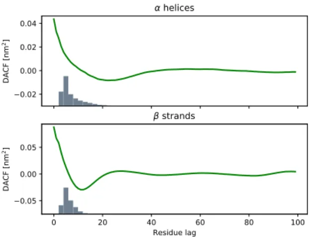
4 0.02 0.00 0.02 0.04 DA CF [n m 2] helices 0 20 40 60 80 100 Residue lag 0.05 0.00 0.05 DA CF [n m 2] strands
FIG. 4: Upper panel: DACFs for the protein axis of well structured proteins containing essentially α-helices and his-togram for the lengths of the latter. Lower panel: The same for β-strands.
can be attributed to the presence of secondary struc-ture elements, in which the direction of the displacements changes periodically with residue lags of approximately 2 (β-strands) to 4 (α-helices). The fact that the oscilla-tions are less pronounced for unstructured proteins than for well-structured ones is simply due to the fact that unstructured proteins contain fewer secondary structure elements.
The DACF for the protein axis of well-structured pro-teins has a striking similarity with the VACF of simple liquids. A surprising result of Rahman’s historic simu-lation of liquid argon22 was that the VACF for such a
system does not decay exponentially, as for the Langevin model, but displays damped oscillations which are as-cribed to rattling motions of the diffusing molecules in the cage of nearest neighbours. The lag time corre-sponding to the first minimum corresponds here to the typical time for a reversal of its velocity. In analogy, the DACF for the protein axis of well-structured pro-teins displays a pronounced minimum for residue lags of about n = 18, which means that the displacement vector d tends to invert its direction after 18 consec-utive steps. The ScrewFrame protein axis may here be considered as an analogue of a simulated (discrete) Molecular Dynamics trajectory. Knowing that typical secondary structure elements have about a length of 18, such a behavior could be explained by the typical “helix-loop-helix” successions in well-structured proteins such as myoglobin. The term “helix” must here be under-stood in the sense of the ScrewFrame algorithm, i.e. as a regular secondary structure element, a category that in-cludes α-helices and β-strands. To investigate this point in more detail, we have computed the DACFs for the pro-tein axis of well-structured propro-teins separately for
sub-0 20 40 60 80 100 Residue lag 0.1 0.0 0.1 0.2 0.3 0.4 0.5 0.6 0.7 Memory function well-structured unstructured
FIG. 5: Memory kernel of the protein axis DACF for well-structured proteins and unwell-structured proteins.
ensembles of protein structures containing, respectively, essentially α-helices and β-strands and recording in both cases histograms for the lengths of these secondary struc-ture elements. Fig. 4 shows clearly that the first min-ima of the axis DACFs are correlated with the maximum lengths of the secondary structure elements, which con-firms the hypothesis that the first minimum of the DACF reflects effectively the recurrent “helix-loop-helix” motif in globular well-structured proteins. Since this motif is less present in IDPs, the minimum of the corresponding protein axis DACF is less pronounced.
The frequency of the “helix-loop-helix” motif should also be reflected in the memory kernel of the DACF. Fig. 5 shows the memory kernels for protein axis DACFs of well-structured proteins and unstructured proteins. Although the difference is small, it is systematic: The memory function corresponding to the DACF of well-structured is systematically larger than its counterpart for unstructured proteins, indicating stronger “folding memory”. The slight oscillations in the latter case should not be overinterpreted since they might be artefacts due to insufficient statistics.
IV. CONCLUSIONS
Our study shows that suitably defined polymer mod-els for proteins enable a meaningful statistical analysis of their folding properties on the basis of “polymer paths”. Each path is here a succession of points that represent the residues, and two types of paths are considered: 1) the Cα-representation, where each residue is represented
by its Cα-atom, and 2) the ScrewFrame representation,
where each residue is represented by the projection of the Cα position onto an appropriately constructed
of the generalized Langevin equation. We show in par-ticular that the memory functions associated with the displacement autocorrelation function along the protein chain display much stronger “folding memory” for well-structured proteins than for IDPs. Although the statisti-cal basis for unstructured proteins is still fairly small, the theoretical framework allows for discriminating between ensembles of well-structured and unstructured proteins. The next step will be to develop suitable simple memory
quantitatively and which have a physical interpretation.
Supplementary Material
See supplementary material for the complete source code of our analysis software with the input and output datasets.
1 R. H. Austin, K. W. Beeson, L. Eisenstein, H.
Frauen-felder, and I. C. Gunsalus, Biochemistry 14, 5355 (1975).
2
N. Alberding, R. H. Austin, S. S. Chan, L. Eisenstein, H. Frauenfelder, I. C. Gunsalus, and T. M. Nordlund, The Journal of Chemical Physics 65, 4701 (1976), ISSN 0021-9606, 1089-7690.
3 H. Hartmann, F. Parak, W. Steigemann, G. Petsko,
D. Ponzi, and H. Frauenfelder, P Natl Acad Sci Usa 79, 4967 (1982).
4 H. Frauenfelder, S. G. Sligar, and P. G. Wolynes, Science
254, 1598 (1991).
5
H. J. Dyson and P. E. Wright, Nature Reviews Molecular Cell Biology 6, 197 (2005), ISSN 1471-0072, 1471-0080.
6 R. B. Best, Current Opinion in Structural Biology 42, 147
(2017), ISSN 0959440X.
7
A. Soranno, A. Holla, F. Dingfelder, D. Nettels, D. E. Makarov, and B. Schuler, Proceedings of the National Academy of Sciences 114, E1833 (2017), ISSN 0027-8424, 1091-6490.
8 P. Kulkarni and V. N. Uversky, PROTEOMICS 18,
1800061 (2018), ISSN 16159853.
9
P. W. Rose, A. Prli, C. Bi, W. F. Bluhm, C. H. Christie, S. Dutta, R. K. Green, D. S. Goodsell, J. D. Westbrook, J. Woo, et al., Nucleic Acids Research (2014).
10
M. Varadi, S. Kosol, P. Lebrun, E. Valentini, M. Black-ledge, A. K. Dunker, I. C. Felli, J. D. Forman-Kay, R. W. Kriwacki, R. Pierattelli, et al., Nucleic Acids Research 42,
D326 (2014), ISSN 0305-1048, 1362-4962.
11
M. Necci, D. Piovesan, Z. Doszt´anyi, P. Tompa, and S. C. E. Tosatto, Bioinformatics 34, 445 (2018), ISSN 1367-4803, 1460-2059.
12
W. Kuhn, Kolloid-Zeitschrift 68, 2 (1934), ISSN 0303-402X, 1435-1536.
13 G. R. Kneller and K. Hinsen, Acta Crystallogr D 71
(2015).
14
P. E. Rouse, The Journal of Chemical Physics 21, 1272 (1953), ISSN 0021-9606, 1089-7690.
15 P. G. de Gennes, The Journal of Chemical Physics 55, 572
(1971), ISSN 0021-9606, 1089-7690.
16
T. C. B. McLeish, Advances in Physics 51, 1379 (2002), ISSN 0001-8732, 1460-6976.
17
A. Papoulis, Probablity, Random Variables, and Stochastic Processes (McGraw Hill, New York, 1991), 3rd ed.
18 J.-M. Chandonia, G. Hon, N. S. Walker, L. Lo Conte,
P. Koehl, M. Levitt, and S. E. Brenner, Nucleic Acids Re-search 32, D189 (2004).
19 N. K. Fox, S. E. Brenner, and J. M. Chandonia, Nucleic
Acids Research 42, D304 (2013).
20
J. Boon and S. Yip, Molecular Hydrodynamics (McGraw Hill, New York, 1980).
21 R. Zwanzig, Nonequilibrium statistical mechanics (Oxford
University Press, 2001).
22
A. Rahman, Physical Review 136, A405 (1964), ISSN 0031-899X.