Potential of Space-Borne LiDAR Sensors for Global Bathymetry in Coastal and Inland Waters

(1)

HAL Id: hal-01521998

https://hal.archives-ouvertes.fr/hal-01521998

Submitted on 12 May 2017

HAL is a multi-disciplinary open access

archive for the deposit and dissemination of

sci-entific research documents, whether they are

pub-lished or not. The documents may come from

teaching and research institutions in France or

abroad, or from public or private research centers.

L’archive ouverte pluridisciplinaire HAL, est

destinée au dépôt et à la diffusion de documents

scientifiques de niveau recherche, publiés ou non,

émanant des établissements d’enseignement et de

recherche français ou étrangers, des laboratoires

publics ou privés.

Potential of Space-Borne LiDAR Sensors for Global

Bathymetry in Coastal and Inland Waters

Hani Abdallah, Jean-Stéphane Bailly, Nicolas Baghdadi, Nathalie

Saint-Geours, Frederic Fabre

To cite this version:

Hani Abdallah, Jean-Stéphane Bailly, Nicolas Baghdadi, Nathalie Saint-Geours, Frederic Fabre.

Po-tential of Space-Borne LiDAR Sensors for Global Bathymetry in Coastal and Inland Waters. IEEE

Journal of Selected Topics in Applied Earth Observations and Remote Sensing, IEEE, 2013, 6 (1),

pp.202 - 216. �10.1109/JSTARS.2012.2209864�. �hal-01521998�

(2)

B

Potential of Space-Borne LiDAR Sensors for Global

Bathymetry in Coastal and Inland Waters

Hani Abdallah, Jean-Stéphane Bailly, Nicolas N. Baghdadi, Nathalie Saint-Geours, and Frederic Fabre

Abstract—This work aimed to prospect future space-borne

LiDAR sensor capacities for global bathymetry over inland and coastal waters. The sensor performances were assessed using a methodology based on waveform simulation. A global representa- tive simulated waveform database is first built from the Wa-LiD (Water LiDAR) waveform simulator and from distributions of water parameters assumed to be representative at the global scale. A bathymetry detection and estimation process is thus applied to each waveform to determine the bathymetric measurement probabilities in coastal waters, shallow lakes, deep lakes and rivers for a range of water depths. Finally, with a sensitivity analysis of waveforms, the accuracy and some limiting factors of the bathymetry are identified for the dominant water parameters. Two future space-borne LiDAR sensors were explored: an ul- traviolet (UV) LiDAR and a green LiDAR. The results show that the bathymetric measurement probabilities at a 1 m depth is 63%, 54%, 24% and 19% with the green LiDAR for deep lakes, coastal waters, rivers and shallow lakes, respectively, and 10%, 22%, 1% and 0% with the UV LiDAR, respectively.

The threshold values of dominant water parameters (sediment, yellow substance and phytoplankton concentrations) above which bathymetry detection fails were identified and mapped. The accu- racy on the bathymetry estimates for both LiDAR sensors is 2.8 cm for one standard deviation with negligible bias (approximately 0.5 cm). However, these accuracy statistics only include the errors coming from the digitizing resolution and the inversion algorithm.

Index Terms—Accuracy, bathymetry, LiDAR, satellite, wave-

form model.

I. INTRODUCTION

ATHYMETRY is the measurement of underwater depth. Bathymetry on coastal and inland waters is important for a wide range of research topics and for a variety of societal needs. In coastal waters, these needs correspond to maritime navigation, ocean circulation modelling [1], ecosystem monitoring [2], tsunami or hurricane risk prevention [3], and marine archaeology [4]. In inland waters, bathymetry mapping is important for navigation and can help efforts to manage and sustain natural resources financially and ecologically [5], [6]. More- over, monitoring the changes in bathymetry in time can be used to identify patterns of fluvial or coastal erosion or deposition to support a process of sustainable management [7], [8].

Water depth can be measured directly with conventional methods by dropping a weighted line into the water, or either indirectly with remote sensing methods [9]. Bathymetric remote sensors mainly include single-beam and Doppler echo sounders [10], [11] or multi-beam SONAR (Sound Navigation And Ranging) (e.g., [12], [13]). Because echo sounder systems are not capable of measuring depth in very shallow water, bathymetry coverage is usually incomplete in coastal and inland waters [14]. As an alternative, optical imagery has been used to estimate water depth, but only in clear water conditions [9], [15], [16].

Despite the use of optical signals, Airborne LiDAR Bathymetry (ALB) systems have proved to be suitable for

mapping bathymetry because of their accuracy and high spatial density features [17]–[19], and they can penetrate waters up to three times deeper than can passive systems [20]. Currently, the operational ALB systems are (i) the Scanning Hydrographic Operational Airborne LiDAR Survey system (SHOALS) man- ufactured by Optech Inc. and under contract to the U.S. Army Corps of Engineers [21], (ii) the HawkEye system from the Swedish Navy and Hydrographic Department [18], (iii) the Australian Laser Airborne Depth Sounder (LADS) [22], and (iv) the Experimental Advanced Airborne Research LiDAR (EAARL) [8]. Most of these ALB detectors use a green laser pulse in their emissions (532 nm) and can register returned waveforms with contributions from the water surface, column and bottom [23]–[25]. A way to estimate water depth from LiDAR waveforms is thus to multiply the half time difference between the water surface and the bottom peaks by the speed of light in the inherent water column [26], [27].

Many studies aimed to quantify bathymetry accuracies from airborne bathymetric LiDAR systems in coastal waters, lakes or rivers. The computed accuracy on the bathymetry estimates ranged between 7 cm and 32 cm for one standard deviation [8], [17], [19], [28], [29], with a maximal depth penetration ranging from 15 to 50 m [19], [29], [30].

However, compared to other remote sensing bathymetric techniques, LiDAR systems have some disadvantages. First, the feasibility of measurements is dependent on water clarity. Some surveys may need to be repeated if water clarity is too low. Secondly, surface waves can generate surface foams which can make bathymetry more difficult. Conversely, specular reflexion of laser beams in the case of flat water surfaces can cause distortion or saturation events and can overload

(3)

the detector [31]. Consequently, most of ALB sensors use a constant off nadir scan angle that also makes the refraction corrections constant. Finally, ALB techniques have limitations to map global near shore bathymetry with regard to reduced spatial coverage and costs. This latter disadvantage leads to the consideration of space-borne bathymetric LiDAR systems.

To date, one space-borne LiDAR sensor has been launched: the Geoscience Laser Altimeter System (GLAS) from ICESat (Ice Cloud and Elevation Satellite). The first objective of this system was to determine the mass balance of the polar ice sheets and their contributions to global sea level change. The second objective was to measure the cloud heights and aerosols in the atmosphere and to map the topography of land surfaces. The second generation of the ICESat orbiting laser altimeter is scheduled for launch in late 2015. The European Space Agency (ESA) plans to launch the Atmospheric Dynamics Mission Aeolus (ADM-Aeolus), based on a Doppler Ultraviolet LiDAR system, in 2013 to perform global wind-component-profile observations [32]. These space-borne LiDAR missions are not dedicated to bathymetric uses.

Consequently, future bathymetric satellite LiDAR mission configurations need to be explored to answer the following questions: What percentage of shallow immersed Earth surfaces can be viewed by a bathymetric satellite LiDAR and at what accuracy? How much does it depend on LiDAR parameters?

One way to investigate these questions is to analyse the performance of satellite LiDAR configurations for bathymetric applications from a database of LiDAR waveforms representative of the physical conditions of the water encountered all over the Earth. However, to produce a database that is representative of all possible physical conditions of the water using different LiDAR configurations would require a huge investment in time, manpower, and money. For these reasons, the use of simulated waveforms provided from LiDAR signal models is an interesting alternative.

Recently, a Water LiDAR simulator (Wa-LiD) was developed to generate LiDAR waveforms for any wavelength in the optical spectrum domain between 300 and 1500 nm [33]. This simulator is based on equations from previous hydrographic LiDAR models [23]–[25], [34] but it integrates radiative transfer laws governed by the physical properties of water for any wavelength. In addition, this simulation model uses a geometrical representation of the water surface with the geometric model of Cook and Torrance [35], and it takes into account both the characteristics of detection noise and the signal level due to solar radiation.

The main objective of this study is to propose a framework that permits estimation of the overall bathymetric performance of satellite LiDAR sensors. Within the proposed framework, the performances of sensors on inland and coastal water types (coastal, river, shallow lake and deep lake waters) are also anal- ysed separately. This framework mainly relies on the exploita- tion of a representative database of water parameters that is used to simulate LiDAR waveforms according to the distributions of water parameter values that are most encountered at the global scale and for each water type.

In this study, two bathymetric LiDAR sensor configurations were investigated. The first emits laser beams in the usual green

wavelength (532 nm) and the second uses the UV wavelength (355 nm). From the usual Nd-YAG lasers (Neodymium-doped Yttrium Aluminium Garnet), the green wavelength is known to offer the highest penetration performance and is therefore the most often used wavelength in airborne LiDAR bathymetry [17], [36]. The UV wavelength can also penetrate clear water despite being more absorbed than the green wavelength [37]. UV has been used to measure ozone and aerosols in the atmosphere, such as the Differential Absorption LiDAR (DIAL) of NASA [38], [39], and forest canopy geometry [40]. An other example of UV LiDAR sensor is the ATLID sensor (ESA’s Satellite-borne Atmospheric LiDAR sensor), designed to provide satellite measurements of cloud-top height both at day and night times [41].

The overall proposed framework is divided into four steps corresponding to the main parts of this paper.

First, the input parameters of the Wa-LiD model are selected and used to generate a simulated LiDAR waveforms database. These parameters are (i) system parameters depending on the two system configurations (e.g., emitted power, pulse width, receiver area, field of view) and (ii) water parameters (e.g., surface and bottom slope, surface rugosity, sediment concentration).

Second, due to the large number of water parameters used in the Wa-LiD model and because of a recently proposed methodology [42], a Global Sensitivity Analysis (GSA) of the Wa-LiD waveforms to water parameters is performed to identify the dominant water parameters that highly influence backscattered waveforms for each type of water.

Third, the waveforms that permit detection of the water bottom are identified through a peak detection method. There- fore, the detection probabilities of the water bottom are computed for the two LiDAR configurations, all water types, and different water depths.

Finally, after using adapted mathematical functions to fit the different contributions of the LiDAR signal (surface, column and bottom), the accuracy of the bathymetry estimates for waveforms with a detectable water bottom is estimated. The signal to noise ratio (SNR) and the threshold values of dominant water parameters for bathymetry are also identified.

II. MATERIALS AND METHODS A. Waveform Simulation

The simulated waveforms used in this study were generated by the Wa-LiD model [33]. The Wa-LiD model integrates both noise due to solar radiation and detector noise, making this model especially suitable for satellite LiDAR mission exploratory studies.

In the Wa-LiD model, the outputs are simulated waveforms received by the LiDAR sensor corresponding to photonic power as a function of time . These waveforms are assumed to be the sum of the echo waveforms backscattered from the successive media encountered by the laser beam [24]:

(1) where denotes the waveform recorded by the detector,

(4)

TABLE I

SENSOR PARAMETER VALUES OF THE TWO INVESTIGATED LIDAR SATELLITE

SENSORS (UV AND GREEN)

denotes the water column contribution waveform, and denotes the bottom contribution waveform. The noise was divided into two sources:

(i) the shot noise contribution coming from solar ra- diations is defined as a Gaussian white noise with parameters depending on the solar irradiance and the Field Of View (FOV) [34], [43]. The solar irradiance was fixed to 0.025 (value for daytime operation [25], [34]). (ii) the detector noise contribution which is co-linear

to all other waveform contributions [33].

However, Wa-LiD does not take into account the atmospheric noise which depends on the attenuation and volume scattering by particles and molecules constituting the atmosphere such as aerosols, water vapor, etc [44], [45].

The equations and parameters interacting in these different power components can be found in detail in Abdallah et al. [33]. The Wa-LiD model simulates each waveform contribution, such as the bottom waveform contribution which is the key information to estimate bathymetry from LiDAR waveforms [26]. Wa-LiD was validated by comparing the simulations to actual airborne or satellite data in the 532 nm and 1064 nm spectra (HawkEye and GLAS): the Wa-LiD model showed a good ability to simulate the observed waveforms by fitting un- known water parameters [33]. However, the Wa-LiD simulations depend on many sensor and water parameters.

1) Sensor Parameters of the Wa-LiD Model: Two bathy-

metric satellite LiDAR configurations were investigated in this study. The first emits laser beams in the usual 532 nm wavelength (green). The second uses the UV wavelength (355 nm).

The values of the instrumental parameters acting in the Wa-LiD equations may or may not depend on the LiDAR wavelength. The retained values of these parameters were chosen with the EADS-Astrium company (European Aero- nautic Defense and Space Company) and listed in Table I. The lowest FOV angle used in simulation reduce highly the solar radiation noise. Consequently our simulated waveforms are slightly noised compared to actual waveforms coming from sensors with higher FOV angles (Fig. 1).

Fig. 1. Simulated 532 nm waveforms with different FOV angles (water depth = 5 m).

2) Water Parameters of the Wa-LiD Model: Four types of in-

land and coastal waters were distinguished in this study: coastal, river, shallow lake and deep lake waters. The optical properties of water are different in shallow and deep lakes because shallow waters are richer in suspended sediments and dissolved organic matter (yellow substances) [46]. Table II presents the range values and distribution laws for water parameters that do not depend on water types. These parameters are connected to the water surface or bottom characteristics. Most of shallow waters in coastal areas have a small bottom slope [47], the steep slope was founded in special case of water bottom for example around the Arctic and can reach 39 [48]. Moreover, it has been shown that slope distribution in rivers usually follows an expo- nential decrease from upstream to downstream [49]. For these reasons, we used the log-normal distribution of (Table II) for all water types centred on a value of 3 that generates little number of high slope values.

Table III shows the range values and the related distribution laws for the water column parameters depending on each water type. The distribution laws and range values of yellow substances , phytoplankton and sediment came from existing databases collected on water bodies around the world (from USGS data collected between 1977 and 1999 and from the SeaWiFS Project of NASA/GSFC (Goddard Space Flight Centre, 1997). The parameter, which corresponds to the co- efficient of specular light backscattered from the water surface, can theoretically vary between 0 and 1, corresponding to totally diffuse or totally specular surfaces, respectively [35]. In this study, a uniform distribution [0.6–0.9] of was chosen arbitrarily in regard to the geometrical representation of the water surface, such as small specular facets in the Cook-Tor- rance model. For the parameter, corresponding to the root mean square error of the surface facet slopes in the Cook-Tor- rance model, a range of 0.1–0.5 was chosen. This range was given by the unique literature of Beckman and Spizzochino [50]. The values of the parameter corresponding to the bottom albedo were given by the literature for different types of bottoms: gravel, sand, limestone, periphyton, debris, cobble, algae and mud [15], [20], [51], [52].

(5)

TABLE II

RANGE VALUES (MINIMUM–MAXIMUM) OF WATER PARAMETERS FOR ALL WATER TYPES

(SURFACE AND BOTTOM SURFACE PARAMETERS). AND DENOTE THE MEAN AND THE STANDARD DEVIATION OF THE LOG-NORMAL DENSITY FUNCTION

TABLE III

RANGE VALUES (MINIMUM–MAXIMUM) OF CONCENTRATIONS OF YELLOW SUBSTANCES AY0, PHYTOPLANKTON CPH AND SEDIMENT S FOR THE FOUR CONSIDERED WATER TYPES

Fig. 2. Yellow substances , phytoplankton and sediment concentration distributions for the four considered water types. and denote the mean and the standard deviation of the fitted log-normal density function (black curve), respectively.

Fig. 2 shows the collected distributions for all Wa-LiD water parameters and for the four types of waters. The sediment concentration varies from 0 to 250 mg/l in the river waters, but only from 0 to 15 mg/l in the deep lake water. Similarly, the histograms come from data collected worldwide [53]. The empir- ical histograms of and were thus fitted with log-normal

density functions (Fig. 2). The fitting process gives the and log-normal law parameter estimates. The phytoplankton concentrations and log-normal distribution parameters ( and

) were more directly given by [61], [62].

The water parameters including all the scene parameters are assumed to be homogeneous within the footprint or FOV area.

(6)

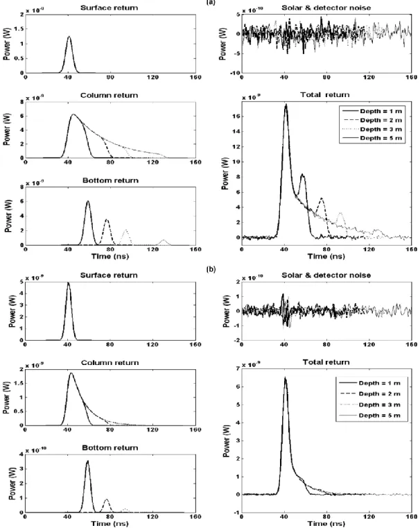
Fig. 3. Simulated LiDAR waveforms in coastal waters for 1, 2, 3 and 5 m water depths. (a) Green wavelength, and (b) UV wavelength. 3) Wa-LiD Simulation Examples: Fig. 3 shows examples of

simulated waveforms for the two studied satellite LiDAR sensors with the sensor parameter values given in Table I. We used in our simulations a simplified theoretical case: the temporal origin of our waveforms was fixed arbitrary. It does not simulate the sensor orbit. Here, the water surface was considered smooth ( , ) and the water bottom was sandy . The water column parameters used in these simulations correspond to the mean coastal water conditions: i) a yellow substances concentration equal to 0.1 , ii) a phytoplankton concentration equal to 8 and iii) a sediment concentration equal to 9 mg/l. Waveforms were generated for water depths equal to

1, 2, 3 and 5 m. As shown in Fig. 3, the bottom peak magnitude in the received waveforms decreases with water depth due to laser beam attenuation along the water column. The green signal penetrates deeper into the water column depending on the water properties and is reflected from the bottom, showing a significant bottom waveform contribution. The UV signal is attenuated in the water column, and the bottom waveform contribution is low for shallow water and disappears for deep water.

Fig. 4 shows the effects of the bottom slope on waveforms. For highest slopes, the bottom echo is highly stretched and its width becomes larger than the width of other echoes (approximately 70 ns for a slope of 35 ).

(7)

Fig. 4. Simulated green LiDAR waveforms in coastal waters for different bottom slope at 2 m depth.

B. Sensitivity Analysis of LiDAR Bottom Contribution Waveforms

A sensitivity analysis will be performed to determine the dominant water parameters on the bottom contribution waveforms that result from the interaction between the laser beam passing through the water surface, the water column and the water bottom. Because an analytical analysis of the Wa-LiD model sensitivity would be difficult, we preferred to use a variance-based method using a quasi Monte-Carlo experimental design of model parameters and producing synthetic and easily interpretable sensitivity indices: the Sobol sensitivity indices [63].

1) Experimental Design: To perform a Sobol sensitivity

analysis of all water parameters on the bottom contribution waveform (except water depth), we used the quasi-random Sobol sampling in the water parameter distributions (Tables II and III), and known to be one of the best random sampling designs for the Sobol sensitivity analysis framework [64], [65]. The design was also stratified among the two sensor configurations (532 and 355 nm) and the four water types (coastal, river, shallow lake and deep lake) for six different depths (1, 2, 3, 5, 10 and 15 m). Forty-eight strata were thus obtained having a set of 10 000 simulated waveforms for each. We thus produced a database of 480 000 Wa-LiD simulated waveforms.

2) Sensitivity Indices: Sobol Indices: To determine the

dominant water parameters, two Sobol sensitivity indices were calculated: the first-order sensitivity index (SI) and the total sensitivity index (TS). We retained as a unique sensitivity indicator because it integrates interactions of parameters in the Wa-LiD model. For given water parameter and a scalar model output Y, the generic formulation of is

(2) where is the variance of and is its expectation. denotes all other parameters but . is the variance of the conditional expectation of Y, having frozen all sources of variation but . Consequently, usually ranges from 0 to 1, and the higher the , the more sensitive the model to .

Fig. 5. Example of Wa-LiD waveform smoothed by the Wiener filter with a detectable bottom. and are the beginning and the end of the time series, respectively; and are the amplitude and the time position of the surface peak; and . are the amplitude and the time position of the bottom peak.

Here, the model output is , which is multidimensional. Therefore, a multivariate global sensitivity analysis method [42] proposed initially by Campbell et al. [66] is used. The principle of this multidimensional Sobol method is i) to decompose the model outputs (waveforms) upon a complete orthogonal basis computed by Principal Component Analysis (PCA) and ii) to compute Sobol indices on each component of the decomposition. Then, a unique Sobol index attached to a water parameter result from the scalar product between the first- order Sobol indices and related eigenvalues from PCA [42].

C. Water Bottom Echo Detection From Wa-LiD Waveforms

The registered LiDAR waveforms allowing bathymetry are usually composed of two main peaks representing the surface and the bottom echoes [17]. To detect the water bottom echo, i.e., the peak from Wa-LiD waveforms, a Wiener filtering was used in a denoising step [67] to smooth the waveform and to facilitate a search of the two peaks (Fig. 5). Second, a peak detection method is applied on the smoothed waveform , and it searches the amplitude and the time position of the first maximum (the instant where ). This maximum should be greater than the maximum of between and (Fig. 5), where is fixed according to a constant distance between the sensor and the water surface. The search for the first maximum proceeds in two ways:

• Forward, from the beginning of the time series

to the end of the time series . The peak found is thus considered to be the surface peak, with amplitude and a time position .

• Backward, from to to find the bottom peak, giving the bottom amplitude and the time position . When the two peaks are found, the waveform is declared to have a detectable bottom. This process permits the identification of waveforms with a detectable water bottom from the simulated waveform database.

To analyse the bathymetric performances of each of the studied sensors, the percentage of waveforms with a detectable

(8)

bottom were calculated for each water type and for different water depths (1, 2, 3, 5, 10 and 15 m).

D. Bathymetry Estimation From Wa-LiD Waveforms

Waveforms presenting a detectable bottom are fitted by mathematical functions. Several functions have been performed in the literature to fit the waveform components, such as two Gaussian curves to approximate both the surface and the bottom returns [26] or three Gaussian curves used [68] to fit the water surface, the water column and the bottom return. Other functions are also used, such as the Weibull distribution and the Burr function, to approximate asymmetric waveforms [69]. Moreover, several combinations of functions were tested by the work of Ceccaldi (Master thesis, 2011) to fit the waveform contributions, but the combination of a Gaussian function, a triangle function and a Weibull function to fit the surface, the column and the bottom echoes, respectively, showed the best fit.

Our algorithm uses the same mixture of functions as follows:

Fig. 6. Fitted simulated waveform with a sum of a Gaussian function (water surface peak), a triangle function (water column) and a Weibull function of water (bottom peak). The estimated depth is 2.9887 m for an actual depth of 3 m.

where is the Gaussian function defined as:

where is the scale factor (amplitude) of the Gaussian, (4)

incidence angle. depend on the incidence angle of the sensor, the water refractive index and the water surface and bottom slope.

Next, the bias , i.e., mean of errors and the stan- dard deviation (SD) between the estimated depth retrieved from is the time position of the surface (ns), and is the standard

deviation.

is the triangle function [70] multiplied by an amplitude and defined as:

waveforms and the actual depth, denoted as , was calculated for each type of water using the usual accuracy statistics:

(5) denote the time positions of triangle vertices.

is the Weibull function multiplied by an amplitude [71]:

(6) is the scale parameter (time position of the bottom in ns) and is the shape parameter.

A nonlinear least-squares (NLS) approach using the Lev- enberg-Marquardt optimisation algorithm [72], [73] was performed to fit the sum of three functions (Fig. 6). The detection method for the amplitudes and time positions (i) of the Gaussian function and (ii) of the Weibull function . The shapes of the Gaussian and Weibull functions are initialised as , where is the emitted pulse width at half maximum. The triangle function amplitude is initialised by . The triangle vertices ,

and are initialised with , respectively. The NLS fitting provides fitted parameter values. The bathymetry estimate could be calculated as follows:

(7)

1) Water Parameter Values Limiting Bathymetry Detection:

The range values of the dominant water parameters were divided into regular intervals (logarithmic scale), and the detection probability was mapped for each dominant water parameter pair. For each interval pair, the detection probability was defined as the ratio between the number of detectable waveforms and the total number of waveforms belonging to these intervals. From these maps, the threshold values of dominant water parameters are identified to delineate detection areas, i.e., areas where the detection probability is greater than zero.

2) Signal to Noise Ratio (SNR): The noise in waveforms

bathymetry. Thus, the ratio between the bottom peak amplitude and the standard deviation of the noise (sum of two noise contributions: ), i.e., the signal to noise ratio, was calculated for each Wa-LiD waveform as:

(8) The distribution of detectable waveforms was calculated for each water type and different water depths. The lowest values that permit the bathymetry to be detected were also identified.

(9)

Fig. 7. Global bathymetry probabilities. (a) Green configuration. (b) UV configuration.

III. RESULTS

A. Global Bathymetry Probability in Coastal and Inland Waters

Using the peak detection method described in method Section II-C, Fig. 7 presents the bathymetric probabilities, i.e., the percentage of waveforms with a detectable water bottom, we can expect from the two studied sensors for all coastal or inland water types. Obviously, the bathymetry probability decreases with water depth whatever the water type. With the green sensor, the bathymetry probability becomes lower than 20% for water depths greater than 5 m in coastal waters and deep lakes (Fig. 7(a)). For rivers and shallow lake waters, the bathymetry probability is lower than 10% for depths higher than 2 m. The results obtained also show that for all water types, the bathymetry probability in the green sensor is more important than that in the UV. For example, the bathymetry probability is 53.5% in the coastal water compared with 22% in the UV (Fig. 7(b)).

With the UV sensor, the bathymetry probability is low for all water types and becomes lower than 10% for water depths greater than 3 m. Moreover, the highest probabilities are obtained for coastal waters, decreasing from 22% at a 1 m water depth down to 3% at 5 m. For river waters and shallow lakes, the bathymetry probability is close to 0 for any water depth (Fig. 7(b)). In deep lakes, the bathymetry probability varies from 10% at 1 m to 1.4% at 3 m.

B. Sensitivity Analysis of Simulated Bottom Echoes

Figs. 8 and 9 present the total sensitivity (TS) indices of the water parameters for the green and UV sensors. The TSs for each of the two system configurations were assessed for the four water types and for six different depths (1, 2, 3, 5, 10 and 15 m). For all water types and for the two system configurations, three water parameters have a negligible impact on the bottom waveforms with TS indices close to 0: the surface slope , the bottom slope and the specular bidirectional reflectance . The results can be summarised as follows (Figs. 8 and 9):

• for coastal waters and with the green LiDAR sensor (Fig. 8(a)), the sediment concentration is the dominant (the most impacting) parameter for all water depths. How- ever, the TS index of the phytoplankton concentration increases with water depth and shows a higher impact from a 10 to 15 m depth. With the UV LiDAR sensor (Fig. 9(a)), the TS indices of are the highest for

Fig. 8. Total Sobol indices related to water parameter variability for green sensor (532 nm) configuration across coastal water, river, deep and shallow lakes and for different depths (1, 2, 3, 5, 10 and 15 m). : surface slope; : bottom slope; : specular bidirectional reflectance; : root mean square of facet slope (water surface roughness); : yellow substances concentration; : sediment concentration; : phytoplankton concentration and : bottom albedo. (a) Coastal water; (b) river; (c) deep lake; (d) shallow lake.

Fig. 9. Total Sobol indices related to water parameter variability for UV sensor (355 nm) across coastal water, river, deep and shallow lakes and for different depths (1, 2, 3, 5, 10 and 15 m). : surface slope; : bottom slope; : specular bidirectional reflectance; : root mean square of facet slope (water surface roughness); : yellow substances concentration; : sediment concentration; : phytoplankton concentration and : bottom albedo. (a) Coastal water; (b) river; (c) deep lake; (d) shallow lake.

all water depths (greater than 0.8 in Fig. 8(a)). For , the TS index increases strongly with the water depth and reaches high values for depths greater than 10 m. For the yellow substances concentration , the TS index decreases with water depth from 0.5 at a 1 m depth to 0 for water depths greater than 5 m. The other water parameters (roughness , bottom reflectance ) show negligible impacts in the UV and green configurations.

• in rivers, and have the highest TS indices for all depths with both UV and green sensor configurations. The TS index of increases with water depth and reaches the

(10)

highest values for depths greater than 5 m with the green sensor (Fig. 8(b)) and greater than 2 m with the UV sensor (Fig. 9(b)). The bottom reflectance shows moderate TS indices (between 0.1 and 0.4 for the green and approximately 0.4 for the UV). The sensitivity of other parameters is very low.

• in deep lakes and for the green configuration (Fig. 8(c)), and show a higher impact on the bottom waveforms for all depths. Moreover, and show high sensitivity indices only for high water depths ( 10 m). For the UV sensor configuration (Fig. 9(c)), shows the most important TS for any depth. For depths greater than 2 m,

and show higher values of TS. The parameter shows remarkable values of TS for depths greater than 3 m. The bottom reflectance shows a negligible impact in the two configurations and for all depths.

• in shallow lakes and for both green and UV LiDAR configurations, the TS indices of , and are the highest for all depths and they increase with water depth. In the UV configuration, the TS values of these three parameters are more important than the values in the green configuration. The roughness and the bottom reflectance show negligible impacts.

C. Water Parameters Limiting Bathymetry

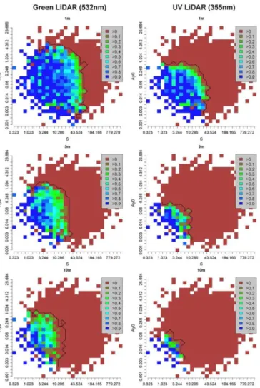
The sensitivity analysis showed that three of the eight water parameters have the highest impact on the bottom waveforms. We therefore hypothesised that these three dominant parameters are the most limiting to bathymetry. Maps of the bathymetry detection were thus produced for dominant parameter pairs for each water type, for each depth and for both sensors using the same simulated waveform database as pre- viously. In the proposed sensitivity analysis study, the bottom slope did not appear as an impacting parameter although it is known that the bottom slope influences strongly the bottom echoes (Fig. 4). Indeed, this is due to the log-normal distribution of used for the waveforms simulations that limit effects of high slopes being lowly probable. Moreover, was performed for a fixed and limited range time in the waveform scale that did not permit to completely take into account the stretching effect of slopes on the bottom echo. For this reason we chose here to also consider bottom slope as a dominant factor. bility in function of parameters, parameters and in function of parameters in coastal waters. The sub-figures present separate results for the green and UV sensors and for 1, 5 and 10 m water depths. For some intervals of water parameters corresponding to low values, the lowest probabilities ( 0.1) are observed. These values are not significant because they correspond to a low number of simulated waveforms in these intervals of water parameters.

The shapes of the probability features on these maps in logarithmic scales are identical (circular and concentric shapes), and they show the interaction of parameter pairs in bathymetry probabilities. The interest of such maps is to identify the parameter threshold that delineates the areas where bathymetry is possible (probability greater than 0) and those where it is not. These maps may be seen as guidelines or abaci that permit

Fig. 10. Maps of bathymetry detection probability according to and distributions in coastal water for 1, 5 and 10 m water depths for green and UV Li- DARs (plotted with logarithmic scale). The black contour corresponds to very low probability values and delineates the bathymetry detection area.

the estimation of bathymetry probability from a space-borne LiDAR sensor on a particular river, lake or littoral environment. These thresholds of dominant water parameter values (sediment, yellow substance and phytoplankton concentrations), above which bathymetry detection fails, are resumed in

For instance, at a 1 m coastal water depth and with green LiDAR, bathymetry cannot be performed when the sediment concentration is higher than 76 mg/l or when the yellow substance concentration is higher than 4.5 mg/l or when the bottom slope is higher than 10 . As a comparison, in 1m depth coastal water and with UV LiDAR, bathymetry cannot be performed when the sediment concentration is higher than 30 mg/l or when the yellow substance concentration is higher than 0.4 mg/l or when the bottom slope is higher than 8 .

D. Bathymetry Accuracy

The waveforms with a detectable bottom were used to determine the water depth using the process detailed in the method section. The errors, i.e., the differences between the water depths retrieved from the fitted waveforms and the actual

(11)

TABLE IV

MAXIMUM OF DOMINANT WATER PARAMETERS (S, , ) CORRESPONDING TO WAVEFORMS WITH DETECTABLE BOTTOMS (--=NO WAVEFORM AVAILABLE

WITH A DETECTABLE BOTTOM WAS FOUND). MAXIMA ARE PRESENTED FOR THE TWO STUDIED LIDAR SENSORS (UV AND GREEN) FOR EACH WATER TYPE

(COASTAL WATERS, RIVERS, DEEP LAKES AND SHALLOW LAKES) AND FOR DIFFERENT WATER DEPTHS (1, 2, 3, 5, 10 AND 15 m)

Fig. 11. Maps of bathymetry detection probability according to and distributions in coastal water for 1, 5 and 10 m water depths for green and UV LiDARs (plotted with logarithmic scale). The black contour corresponds to very low probability values and delineates the bathymetry detection area.

depths used for simulation, were calculated. Therefore, the usual error statistics, that is, the mean of errors (bias) and the

Fig. 12. Maps of bathymetry detection probability according to and distributions in coastal water for 1, 5 and 10 m water depths for green and UV LiDARs (plotted with logarithmic scale). The black contour corresponds to very low probability values and delineates the bathymetry detection area.

standard deviation of errors (SD) were also computed. These statistics can be summarised as follows (Fig. 13).

(12)

Fig. 13. Statistics on the bathymetry estimation errors: bias and standard devi- ations. (a) Green configuration; (b) green configuration; (c) UV configuration; (d) UV configuration.

For the green configuration, the bias ranges from 0.1 to 1.2 cm (Fig. 13(a)), with an SD between 1.7 and 5.0 cm (Fig. 13(b)). The over-estimations of the bathymetry observed in the river water at a 10 m depth and in the shallow lake water at a 5 m depth correspond to two cases where the percentage of detectable waveforms is very low (0.30% and 0.33%, respectively). Therefore, this overestimation related to low number of data is not significant.

For the UV sensor, the bias ranges from 0.4 to 2.0 cm (Fig. 13(c)), with SD values between 1.0 and 4.7 cm (Fig. 13(d)). An underestimation of the water depth was also observed for all water types and at all depths except in coastal water at a 10 m depth. The overestimation of the bathymetry observed for coastal water at a 10 m depth due to the lowest percentage (0.9%) of detectable waveforms is also considered non-significant.

E. Signal to Noise Ratio (SNR) of Bottom Echoes in Waveforms With a Detectable Bottom

The signal to noise ratio (SNR) for bathymetry is defined here by the ratio of the bottom peak amplitude in the waveforms to the noise amplitude. To determine the distribution of SNRs for each water type and water depth, it was calculated for each simulated waveform with a detectable bottom. The minimum and maximum SNRs were calculated for each case in using the two studied LiDAR sensors (Table V).

The SNR values obviously decrease with water depth in the green and the UV configurations for all water types.

Fig. 14 shows a sample of SNR boxplots in coastal water. For the green waveforms, the median of the SNR decreases with water depth from 358 at a 1 m water depth up to 21 at a 15 m water depth (Fig. 14(a)). For the UV waveforms, the median SNR decreases from 155 at a 1 m water depth up to 0 at a 15 m water depth (Fig. 14(b)). However, the most important task from the SNR calculation is to identify the lowest SNR values allowing bathymetry.

TABLE V

MINIMUM AND MAXIMUM OF SNRS CORRESPONDING TO WAVEFORMS WITH

DETECTABLE BOTTOMS. (--=NO WAVEFORM WITH DETECTABLE BOTTOM WAS

FOUND AT THIS DEPTH FOR THIS WATER TYPE)

Fig. 14. Boxplots of SNRs (logarithmic scale) for waveforms with detectable bottoms at 1, 2, 3, 5, 10 and 15 m water depths in coastal waters for the green and UV sensors. (a) Green configuration; (b) UV configuration.

IV. DISCUSSIONS A. Green or UV Space-Borne LiDAR Mission

The two sensor configurations used in this study are ap- proachable with advanced technologies in the next few years (personal communication from the Astrium-EADS company, a European company in space transportation, satellite systems and services). All ALB systems use the 532 nm wavelength because it is the Nd-YAG derivative wavelength that most deeply penetrates turbid waters. Obviously, this is the space-borne sensor that gave the best overall performance. In comparison, to date the UV was not used for bathymetry in coastal and inland waters. However, with the used configuration in this study, the results show the interest of the UV configuration in clear coastal waters and deep lakes and for very shallow water depths. Moreover, these results on the UV sensor capacities could be improved by using higher laser emitted power since there is still room to increase this emitted power according to

(13)

Regarding the SNR values, the bottom peak amplitude without noise in the UV is lower than that in the green (approximately 40 times at a 1 m water depth). At the opposite, the noise power defined as the sum of the solar radiation noise and the detector noise is five times greater in the green than in the UV configuration. Consequently, the SNR values corresponding to LiDAR green waveforms are also obviously higher than those for the UV.

The main advantage of the UV sensor is its ability to be used for multiple applications, including bathymetry, forestry [40] and atmospheric sciences [74]. However, if future technologies with other high frequency pumped laser emerges, blue wavelength LiDAR (450 nm) should also be an interesting alternative for bathymetry [75].

B. Other Factors Affecting Space-Borne Bathymetry

First, the bed morphology of all water types used in simulations is considered as a sloped plane with various slope values. Indeed, more complex morphologies of the bed (micro-geometry, algae presence, etc) within laser footprints may occur which provide additional uncertainty in bathymetry estimation and decrease the overall bathymetry probability results.

In addition, we assumed that the distributions of water parameters were consistent across the depth of water (one layer) and independent of each other.

Second, future works should include the atmospheric effects in the LiDAR signal simulations.

Third, the main limitation of spaceborne LiDARs is the mission’s lifetime related to the laser shot number emitted in the operational period of LiDAR. Therefore, it will be difficult to obtain data with a high spatial density and a high revisit time from spaceborne LiDAR. In coastal waters, where the bathymetry varies very strongly with distance from the coast, a low spacing between successive footprints is necessary for cor- rectly mapping the bathymetry. However, these other aspects of the LiDAR mission configuration should also be explored in future works.

C. Bathymetry Accuracy From Space-Borne LiDARs

Firstly, the used digitizing frequency is of 1 GHz which corresponds to a depth resolution of about 11.4 cm. This is the usual digitizing frequency of airborne sensors and GLAS sensors. The magnitude of errors due to this digitizing resolution for the explored depths (1 m, 2 m, 3 m, 5 m, 10 m, 15 m) is of the same order that the computed accuracy. Consequently, the obtained accuracy statistics on the bathymetry estimations (standard deviation of random error and bias) mainly corresponds to the errors due to digitizing resolution and fitting method errors (inversion). These accuracy statistics are also depending on the distribution of explored depths.

Moreover, in actual data, there are other error budget items to consider which are neglected here. These additional errors come from GPS positioning of the satellite, the geometry of the laser beam, atmospheric conditions, scene complexity (presence of vegetation), etc [76], [77]. Indeed, the overall accuracy (here standard deviation of the random error) of the bathymetry results on the addition of variances of these different error items. For instance, these error items are:

— Errors of about 5 cm due to GPS positioning of the sensor [78].

— Errors of about 2 cm due to pointing error of the laser beam which are for satellite at 600 km height and a near nadir laser beam [79].

— Errors of about 4 cm due to atmosphere which acts to dis- tort the path of the laser pulse as it travels to the target and back again and produce timing errors [78], [80].

The sum of these some error budget items is coherent with accuracy studies on ICESat errors founded in literature on flat and non-complex surfaces [81], [82].

For ALB, larger errors may come from higher pointing errors due to higher incidence angles, and higher platform positioning errors. Accuracy from for ALB manufacturers is about 25 cm [18]. However, the lower noise in the waveforms due to space detector technology allows to expect more accurate statistics than the one observed in experiments from ALB sensors [8], [19], [26].

Another limitation in this study comes from the peak detection method, which is not suitable for very shallow waters ( 1 m) or more noisy waveforms whatever the depth is. For very shallow waters or other sensor configurations (higher FOV angles for example), other waveform processing methods should be developed.

The proposed algorithm is not generic and would surely fail to estimate bathymetry from more noisy waveforms. But, the lowest SNR values allowing bathymetry is approximately 1.1, which corresponds to theory [44] and proves that the proposed the algorithm is efficient for slightly noised LiDAR waveforms.

Moreover, the slight underestimation of the bathymetry observed for both the green and the UV may be also due to the triangle mathematical function used to fit the water column that slightly translates the positioning of the Gaussian function used to fit the bottom echo. Finally, the highest observed in coastal water at a depth greater than 2 m should be related to the low number of data.

V. CONCLUSIONS AND PERSPECTIVES

This work aimed to prospect future space-borne LiDAR sensors capacities for global bathymetry over inland and coastal waters. Two future space-borne LiDAR sensors were explored: an ultraviolet (UV) LiDAR and a green LiDAR emitting at 355 and 532 nm, respectively. The sensor performances were assessed from a methodology based only on waveform simulation. A wide waveform database was first built from the existing Wa-LID waveform simulator and from an experimental design representing observed distributions of water parameters from the literature assumed to be representative at the global scale. A bathymetry detection and estimation process based on Wiener filter and mathematical function fitting were applied to each waveform to determine i) the bathymetry detection rate (bathymetry probability) in coastal waters, shallow lakes, deep lakes and rivers for a range of water depths and ii) the expected bathymetry accuracies. Finally, by using a sensitivity analysis of waveforms, some limiting factors in bathymetry were identified and mapped for the most dominant water parameters.

The results show that the bathymetry probabilities (i.e., bathymetry detection rates) at a 1 m depth are 63%, 54%, 24%

(14)

and 19% with the green LiDAR for deep lakes, coastal waters, rivers and shallow lakes, respectively, and 10%, 22%, 1% and 0%, respectively, with the UV LiDAR. Obviously, the detection rates for UV LiDAR are always lower than for green LiDAR, and the rates decrease when the water depth increases. At a 10 m depth, the bathymetry probability becomes 5%, 8%, 0% and 0% with the green LiDAR for deep lakes, coastal waters, rivers and shallow lakes, respectively. When the bathymetry is detectable, its accuracy for both sensors is approximately 2.8 cm for one standard deviation with a small underestimation (approximately 0.5 cm). These accuracy statistics only include the errors coming from the digitizing resolution and the inversion algorithm.

The sensitivity analysis results indicate three dominant water parameters, which are all related to water column properties: sediment, yellow substances and phytoplankton concentrations. Maps of bathymetry probability were made for each dominant water parameter pair, each water type, and each water depth. These maps allow us to identify the thresholds of dominant water parameters above which bathymetry detection fails. These maps are thus guidelines to estimating bathymetry probability from a space-borne LiDAR sensor on a particular river, lake or littoral environment.

The innovation of this paper mainly comes from the proposed global methodology chaining different compartments: signal modelling, experimental design, sensitivity analysis and signal inversion. This methodology should be considered as a starting point to explore the global performances and limiting factors of any future space-borne LiDAR sensor totally or partially dedicated to bathymetry. Of course, it still exists many limitations in each methodological compartment but the global results permit to identify and rank these limitations which should be the points to be improved in future works. For instance, the sensor performances are strongly related to the representativeness of the waveform database at the global scale and, thus, to water parameter distributions. Here, we assumed that the distributions of the water parameters were homogeneous for any water depth. This assumption is certainly not entirely true, and it should be refined in future works. For other water parameters, such as water surface roughness or water specular coefficients, experiments and ground data acquisition are needed for a better estimation of distributions. This is true for all other parameters: there is a need to build or feed global databases on these parameters that will en- sure better performance assessments. However, the proposed methodology in this paper is already capable of exploring other sensor configurations (e.g., the blue wavelength) for future bathymetric satellite LiDAR mission exploration.

ACKNOWLEDGMENT

The authors would like to thank Yves Pastol from SHOM (French Naval Hydrographic and Oceanographic Service) for his useful advice.

REFERENCES

[1] A. F. Blumberg and G. L. Mellor, “A description of a three-dimen- sional coastal ocean circulation model,” in Three-Dimensional Coastal

Ocean Models, N. Heaps, Ed. Washington, DC: American Geophys-

ical Union, 1987, pp. 1–16.

[2] J. Ferreira, C. Vale, C. Soares, F. Salas, P. Stacey, and S. Bricker, “Monitoring of coastal and transitional waters under the E.U.,” Water

Framework Directive Environ. Monit. Assess., vol. 135, pp. 195–216,

2007.

[3] N. A. Duong, F. Kimata, and I. Meilano, “Assessment of bathymetry effects on tsunami propagation in Viet Nam,” Namadu J., vol. 9, no. 6, pp. 1–9, 2008.

[4] K. Westley, R. Quinn, W. Forsythe, R. Plets, T. Bell, S. Benetti, F. McGrath, and R. Robinson, “Mapping submerged landscapes using multibeam bathymetric data: A case study from the north coast of Ireland,” Int. J. Nautical Archaeology, vol. 40, no. 1, pp. 99–112, 2011.

[5] J. Gao, “Bathymetric mapping by means of remote sensing: Methods, accuracy and limitations,” Progress in Physical Geography, vol. 33, pp. 103–116, 2009.

[6] A. M. Duda and M. T. El-Ashry, “Addressing the global water and environment crises through integrated approaches to the management of land, water and ecological resources,” Water International, vol. 25, no. 1, pp. 115–126, 2000.

[7] S. N. Lane, R. M. Westaway, and D. M. Hicks, “Estimation of erosion and deposition volumes in a large gravel-bed, braided river using syn- optic remote sensing,” Earth Surface Processes and Landforms, vol. 28, no. 3, pp. 249–271, 2003.

[8] P. J. Kinzel, C. W. Wright, J. M. Nelson, and A. R. Burman, “Evalua- tion of an experimental LiDAR for surveying a shallow, braided, sand bedded river,” J. Hydraul. Eng., vol. 133, no. 7, pp. 838–842, 2007. [9] D. Feurer, J. S. Bailly, C. Puech, Y. LeCoarer, and A. Viau, “Very high

resolution mapping of river immersed topography by remote sensing,”

Progress in Physical Geography, vol. 32, no. 4, pp. 1–17, 2008.

[10] T. B. Vermeyen, “Using an ADCP, depth sounder, and GPS for bathy- metric surveys,” in Proc. World Environmental and Water Resources

Congress, Omaha, Nebraska, May 21–25, 1996.

[11] R. L. Dinehart and J. R. Burau, “Repeated surveys by acoustic Doppler current profiler for flow and sediment dynamics,” J. Hydrol., vol. 314, pp. 1–21, 2005.

[12] L. J. Poppe, S. D. Ackerman, E. F. Doran, A. L. Beaver, J. M. Crocker, and P. T. Schattgen, “Interpolation of Reconnaissance Multibeam Bathymetry From North-Central Long Island Sound,” U.S. Geological Society, Open File Report 2005-1145, 2006.

[13] R. L. Ferrari, “Folsom Lake Sedimentation Study,” Technical Service Centre, Denver, CO, Bureau of Reclamation Report, 2005.

[14] H. Wirth and T. Brüggemann, “The development of a multiple trans- ducer multi-beam echo sounder system for very shallow waters,” FIG Working Week, Bridging the Gap Between Cultures, Marrakech, Mo- rocco, May 18–22, 2011.

[15] J. Legleiter, A. Roberts, and L. Rick, “Spectrally based remote sensing of river bathymetry,” Earth Surface Processes and Landforms, vol. 34, pp. 1039–1059, 2009.

[16] M. A. Fonstad and W. A. Marcus, “Remote sensing of stream depths with hydraulically assisted bathymetry (HAB) models,” Geomor-

phology, vol. 72, no. 1–4, pp. 320–339, 2005.

[17] G. C. Guenther, A. G. Cunningham, P. E. LaRocque, and D. J. Reid, “Meeting the accuracy challenge in airborne LiDAR bathymetry,” in

Proc. 20th EARSeL Symp.: Workshop on LiDAR Remote Sensing of Land and Sea, Dresden, Germany, Jun. 16–17, 2000.

[18] R. C. Hilldale and D. Raff, “Assessing the ability of airborne LiDAR to map river bathymetry,” Earth Surface Processes and Landforms, vol. 33, no. 5, pp. 773–783, 2007.

[19] J. S. Bailly, Y. Le Coarer, P. Languille, C. J. Stigermark, and T. Allouis, “Geostatistical estimations of bathymetric LiDAR errors on rivers,”

Earth Surface Process and Landforms, vol. 35, pp. 1199–1210, 2010.

[20] S. Peeri, J. V. Gardner, L. G. Ward, and J. R. Morrison, “The seafloor: A key factor in LiDAR bottom detection,” IEEE Trans. Geosci. Remote

Sens., vol. 49, no. 3, pp. 1150–1157, 2011.

[21] J. L. Irish and W. J. Lillycrop, “Scanning laser mapping of the coastal zone: The SHOALS system,” ISPRS J. Photogramm. Remote Sens., vol. 54, no. 2–3, pp. 123–129, 1999.

[22] A. Cunningham, W. J. Lillycrop, G. C. Guenther, and M. Brooks, “Shallow water laser bathymetry: Accomplishments and applications,” in Proc. XVth Oceanology Int. Exhibition & Conf., Brighton, UK, 1998, vol. 3, pp. 277–288.

[23] J. Feigels, “LiDARs for oceanological research: Criteria for compar- ison, main limitations, perspectives,” Ocean Optics XI, vol. 1750, pp. 473–484, 1992.

[24] H. M. Tulldahl and K. O. Steinvall, “Analytical waveform generation from small objects in LiDAR bathymetry,” Appl. Opt., vol. 38, no. 6,

(15)

[25] H. M. Tulldahl and K. O. Steinvall, “Simulation of sea surface wave influence on small target detection with airborne laser depth sounding,”

Appl. Opt., vol. 42, no. 12, pp. 2462–2483, 2004.

[26] T. Allouis, J.-S. Bailly, Y. Pastol, and C. Le Roux, “Comparison of LiDAR waveform processing methods for very shallow water bathymetry using Raman, near-infrared and green signals,” Earth

Surface Process and Landforms, vol. 35, pp. 640–650, 2010.

[27] S. Peeri and W. Philpot, “Increasing the existence of very shallow- water LiDAR measurements using the red-channel waveforms,” IEEE

Trans. Geosci. Remote Sens., vol. 45, no. 5, pp. 1217–1223, 2007.

[28] C. Flener, E. Lotsari, P. Alho, and J. Käyhkö, “Comparison of empir- ical and theoretical remote sensing based bathymetry models in river environments,” River Research and Applications, vol. 28, no. 1, pp. 118–133, 2012.

[29] G. J. Perry, “Post-processing in laser airborne bathymetry systems,” in

Proc. ROPME/PERSGA/IHB Workshop on Hydrographic Activities in the ROPME Sea Area and Red Sea, Kuwait, October 24–27, 1999.

[30] W. J. Lillycrop, L. E. Parson, J. L. Irish, and M. W. Brooks, “Hydro- graphic surveying with an airborne LiDAR survey system,” presented at the 2nd Int. Airborne Remote Sensing Conf. Exhibition, San Fran- cisco, CA, Jun. 24–27, 1996.

[31] X. Sun, J. B. Abshire, D. Yi, and H. A. Fricker, “ICESat receiver signal dynamic range assessment and correction of range bias due to satura- tion,” EOS Trans. AGU, vol. 86, no. 52, 2005.

[32] D. T. Kokkinos, G. Tzeremes, and E. Armandillo, “Determination of backscatter ratio and depolarization ratio by mobile LiDAR measurements in support of EARTHCARE and AEOLUS missions,” presented at the Workshop on LiDAR Measurements in Latin America, 2011. [33] H. Abdallah, N. Baghdadi, J. S. Bailly, Y. Pastol, and F. Fabre, “Wa-

LiD: A new LiDAR simulator for waters,” IEEE Geosci. Remote Sens.

Lett., vol. 9, no. 5, pp. 744–748, 2012.

[34] G. C. Guenther, “Airborne Laser Hydrography, System Design and Performance Factors,” National Oceanic and Atmospheric Adminis- tration, Rockville, MD, NOAA Professional Paper Ser. NOS1, 1985. [35] R. L. Cook and K. E. Torrance, “A reflectance model for computer

graphics,” ACM Trans. Graphics, vol. 1, pp. 7–24, 1982.

[36] R. A. Smith, J. L. Irish, and M. Q. Smith, “Airborne LiDAR and airborne hyperspectral imagery: A fusion of two proven sensors for improved hydrographic surveying,” in Proc. Canadian Hydrographic

Conf. 2000, Montreal, Canada, p. 10.

[37] A. Bricaud, A. Morel, and L. Prieur, “Absorption by dissolved organic matter of the sea (yellow substance) in the UV and visible domains,”

Limnology and Oceanography, vol. 26, no. 1, pp. 43–53, 1981.

[38] Z. Liu, I. Matui, and N. Sugimoto, “High-spectral-resolution LiDAR using an iodine absorption filter for atmospheric measurements,” Opt.

Eng., vol. 38, pp. 1661–1670, 1999.

[39] E. V. Browell, S. Ismail, and W. B. Grant, “Differential absorption LiDAR (DIAL) measurements from air and space,” Appl. Phys. B:

Lasers Opt., vol. 67, no. 4, pp. 399–410, 1998.

[40] T. Allouis, S. Durrieu, P. Chazette, J.-S. Bailly, J. Cuesta, C. Véga, P. Flamant, and P. Couteron, “Potential of an ultraviolet, medium-foot- print LiDAR prototype for retrieving forest structure,” ISPRS J. Pho-

togramm. Remote Sens., vol. 66, no. 6, pp. S92–S102, 2011.

[41] D. Morancais, R. Sesselmann, G. Benedetti-Michelangeli, and M. Hueber, “The atmospheric LiDAR instrument (ATLID),” Acta Astro-

nautica, vol. 34, pp. 63–67, 1994.

[42] M. Lamboni, D. Makowski, S. Lehuger, B. Gabrielle, and H. Monod, “Multivariate global sensitivity analysis for dynamic crop models,”

Field Crops Research, vol. 113, no. 3, pp. 312–320, 2009.

[43] T. K. Cossio, K. C. Slatton, W. E. Carter, K. Y. Shrestha, and D. Harding, “Predicting small target detection performance of low-SNR airborne LiDAR,” IEEE J. Sel. Topics Appl. Earth Observ. Remote

Sens. (JSTARS), vol. 3, no. 4, pp. 672–688, 2010.

[44] M. S. Belen’kii, “Effect of atmospheric turbulence on heterodyne LiDAR performance,” Appl. Opt., vol. 32, pp. 5368–5372, 1993. [45] R. Agishev, A. Comeron, B. Gross, F. Moshary, S. Ahmed, and A.

Gilerson, “Application of the method of decomposition of LiDAR signal-to-noise ratio to the assessment of laser instruments for gaseous pollution detection,” Appl. Phys. B, vol. 79, no. 2, pp. 255–264, 2004. [46] M. Rijkeboer, A. G. Dekker, and H. J. Gons, “Subsurface irradiance

reflectance spectra of inland waters differing in morphometry and hy- drology,” Aquat. Ecol., vol. 31, pp. 313–323, 1998.

[47] J. B. Keller, “Shallow-water theory for arbitrary slopes of the bottom,”

J. Fluid Mech., vol. 489, pp. 345–348, 2003.

[48] F. Wobus, G. I. Shapiro, M. A. Maqueda, and J. M. Huthnance, “Nu- merical simulations of dense water cascading on a steep slope,” J. Ma-

rine Research, vol. 69, no. 2–3, pp. 391–415, 2011.

[49] L. Leopold and T. Maddock, “The hydraulic geometry of stream chan- nels and some physiographic implications,” U.S. Geol Surv. Prof. Pap., vol. 252, pp. 9–16, 1953.

[50] P. Beckmann and A. Spizzochino, The Scatter of Electromagnetic

Waves From Rough Surfaces. Norwood, MA: Artech House, 1987.

[51] E. J. Hochberg, M. J. Atkinson, and S. Andrefouet, “Spectral reflectance of coral reef bottom-types worldwide and implications for coral reef remote sensing,” Remote Sens. Environ., vol. 85, pp. 159–173, 2003.

[52] D. R. Lyzenga, “Passive remote-sensing techniques for mapping water depth and bottom features,” Appl. Opt., vol. 17, pp. 379–383, 1978. [53] J. T. O. Kirk, Light and Photosynthesis in Aquatic Ecosystems, 3rd

ed. Cambridge, U.K.: Cambridge Univ., 2011, p. 662.

[54] C. D. Mobley, Light and Water: Radiative Transfer in Natural Wa-

ters. San Diego, CA: Academic, 1994.

[55] L. Sipelgas, H. Arst, U. Raudsepp, T. Kouts, and A. Lindfors, “Optical properties of coastal waters of north western Estonia: In situ measure- ments,” Boreal Environ. Res., vol. 9, no. 5, pp. 447–456, 2004. [56] J. A. Warrick, L. A. K. Mertes, D. A. Siegel, and C. Mackenzie, “Esti-

mating suspended sediment concentrations in turbid coastal waters of the Santa Barbara Channel with SeaWiFS,” Int. J. Remote Sens., vol. 25, pp. 1995–2002, 2004.

[57] L. C. Bowling, “Optical properties, nutrients and phytoplankton of freshwater coastal lakes in south-east Queensland,” Aust. J. Mar.

Freshwater Res., vol. 39, pp. 805–815, 1998.

[58] A. A. Gitelson, R. Khanbilvardi, B. Shteinman, and Y. Yacobi, “Re- mote estimation of phytoplankton distribution in aquatic ecosystems engineering construction and operations in challenging environments earth and space,” in Proc. 9th Biennial ASCE Aerospace Div. Int. Conf., 2004, pp. 255–262.

[59] D. H. Jewson and J. A. Taylor, “The influence of turbidity on net phy- toplankton photosynthesis in some Irish lakes,” Freshwater Biol., vol. 8, pp. 573–584, 1978.

[60] M. A. Moline, T. K. Frazer, R. Chant, S. Glenn, C. A. Jacoby, J. R. Reinfelder, J. Yost, M. Zhou, and O. Schofield, “Biological responses in a dynamic buoyant river plume,” Oceanography, vol. 21, no. 4, pp. 70–89, 2008.

[61] M. L. Laanen, “Improving the remote sensing of coloured dissolved organic matter in inland freshwaters,” Doctoral dissertation, Earth and Life Sciences, Vrije University, Amsterdam, The Netherlands, 2007.

[62] P. Cipollini and G. Corsini, “The effect of yellow substance on pigment concentration retrieval using ‘blue to green’ ratio,” in Proc.

IEEE Int. Geoscience and Remote Sensing Symp., IGARSS’94, 1994,

pp. 772–777.

[63] I. M. Sobol, “Sensitivity estimates for non linear mathematical models,” Mathematical Modelling and Computational Experiments, vol. 1, pp. 407–414, 1994.

[64] P. Bratley and B. Fox, “Implementing Sobol’s quasi random sequence generator,” ACM Trans. Mathematical Software, vol. 14, no. 1, pp. 88–100, 1998.

[65] S. Tarantola and M. Koda, “Improving random balance designs for the estimation of first order sensitivity indices,” Procedia—Social and Be-

havioral Sciences, vol. 2, no. 6, pp. 7753–7754, 1997.

[66] K. Campbell, M. D. McKay, and B. J. Williams, “Sensitivity analysis when model outputs are functions,” Reliability Engineering and System

Safety, vol. 91, pp. 1468–1472, 2006.

[67] B. Jutzi and U. Stilla, “Range determination with waveform recording laser systems using a Wiener filter,” ISPRS J. Photogramm. Remote

Sens., vol. 61, no. 2, pp. 95–107, 2006.

[68] B. Long, A. Cottin, and A. Collin, “What Optech’s bathymetric LiDAR sees underwater,” in Proc. IEEE Int. Geoscience and Remote Sensing

Symp., Jul. 23–28, 2007, pp. 3170–3173.

[69] C. Mallet, F. Lafarge, F. Bretar, U. Soergel, and C. Heipke, “LiDAR waveform modelling using a marked point process,” in Proc. Int. Conf.

Image Processing, ICIP, 2009, pp. 1713–1716.

[70] M. Evans, N. Hastings, and B. Peacock, “Triangular Distribution,” in

Statistical Distributions, 3rd ed. New York: Wiley, 2000, ch. 40, pp.

187–188.

[71] P. Rosin and E. Rammler, “The laws governing the fineness of pow- dered coal,” J. Inst. Fuel, vol. 7, pp. 29–36, 1933.

[72] M. A. Hofton, J. B. Minster, and J. B. Blair, “Decomposition of laser altimeter waveforms,” IEEE Trans. Geosci. Remote Sens., vol. 38, no. 4 II, pp. 1989–1996, 2000.

[73] J. Reitberger, P. Krzystek, and U. Stilla, “Analysis of full waveform LiDAR data for the classification of deciduous and coniferous trees,”

(16)

[74] M. Imaki and T. Kobayashi, “Ultraviolet high-spectral-resolution Doppler LiDAR for measuring wind field and aerosol optical proper- ties,” Appl. Opt., vol. 44, pp. 6023–6030, 2005.

[75] A. Morel, B. Gentili, H. Claustre, M. Babin, A. Bricaud, J. Ras, and F. Tièche, “Optical properties of the ‘clearest’ natural waters,” Limnology

and Oceanography, vol. 52, no. 1, pp. 217–229, 2007.

[76] M. E. Charlton, A. R. G. Large, and I. C. , “Application of airborne LiDAR in river environments: The River Coquet, Northumberland, U.K.,” Earth Surface Processes and Landforms, vol. 28, pp. 299–306, 2003.

[77] R. F. Brinkman and C. O’Neill, “LiDAR and photogrammetric map- ping,” The Military Engineer, May–Jun. 2000.

[78] H. J. Zwally, B. Schutz, W. Abdalati, J. Abshire, C. Bentley, A. Brenner, J. Bufton, J. Dezio, D. Hancock, D. Harding, T. Herring, B. Minster, K. Quinn, S. Palm, J. Spinhirne, and R. Thomas, “ICESat’s laser measurements of polar ice, atmosphere, ocean, and land,” J.

Geodynam., vol. 34, no. 3–4, pp. 405–445, 2002.

[79] T. J. Urban, B. E. Schutz, and A. L. Neuenschwander, “A survey of ICESat coastal altimetry applications: Continental coast, open ocean island, and inland river,” Terrestrial, Atmospheric and Oceanic Sci-

ences, vol. 19, no. 1–2, pp. 1–19, 2008.

[80] J. W. Marini and C. W. Murray, “Correction of Laser Range Tracking Data for Atmospheric Refraction at Elevation Angles Above 10 ,” NASA Technical Report, 1973.

[81] H. Abdallah, J.-S. Bailly, N. Baghdadi, and N. Lemarquand, “Im- proving the assessment of ICESat water altimetry accuracy accounting for autocorrelation,” ISPRS J. Photogramm. Remote Sens., vol. 66, no. 6, pp. 833–844, 2011.

[82] J. W. Chipman and T. M. Lillesand, “Satellite-based assessment of the dynamics of new lakes in southern Egypt,” Int. J. Remote Sens., vol. 28, no. 19, pp. 4365–4379, 2007.