Development of a method for controlled cartilage deformation

(1)

Development of a Method for

Controlled Cartilage Deformation

by

Jennifer A. Cooper

B.S. Engineering -Trinity College, Hartford, CT, 1998

SUBMITTED TO THE DEPARTMENT OF MECHANICAL ENGINEERING IN PARTIAL FULFILLMENT OF THE REQUIREMENTS FOR THE DEGREE OF

MASTER OF SCIENCE IN MECHANICAL ENGINEERING

AT THE

MASSACHUSETTS INSTITUTE OF TECHNOLOGY

SEPTEMBER 2000

and to distribute publicly paper and electronic copies of this thesis document in whole or in part.

Author...

6/

(-Department of Mechanical Engineering

$ August 21, 2000

C ertified by ... ... . ....

Brian D. Snyder Assistant Professor of Orthopedic Surgery, Harvard Medical School Thesis Supervisor

Certified by... ...

Derek Rowell Professor of Mechanical Engineering Thesis Supervisor

Accepted by...

Ain A. Sonin Chairman, Department Committee on Graduate Students

BARKER

MASSACHUSETTS INSTITUTE OF TECHNOLOGY

SEP 2

0

2000

(2)

Development of a Method for

Controlled Cartilage Deformation

by

Jennifer A. Cooper

Submitted to the Department of Mechanical Engineering in partial fulfillment of the requirements for the degree of

Master of Science in Mechanical Engineering

Abstract

Hip dysplasia affects as much as 2.8% of infants born, and left untreated accounts for as much as 76% of all cases of hip joint osteoarthritis. Identification of hip dysplasia is fairly arbitrary since there is not a defined procedure for diagnosis. Since hyaline cartilage is slow to regenerate, tissue engineering alternatives have not yet been perfected, and arthroplasty failure occurrs 10 to 15 years following implantation, one of the best treatment options in younger and active patients with abnormal hip geometry remains surgical intervention. The development of an objective function, whereby a surgeon could straightforwardly prescribe the appropriate reconstruction technique, could be an important step to better understanding hip dysplasia and its role in the development of OA.

This thesis proposes a reconsideration of the terms used to quantify and describe hip abnormality. A hypothesis for an objective function for surgical planning, and the development of the testing apparatus and protocol for the validation of this hypothesis are presented.

Thesis Supervisor: Brian D. Snyder

Title: Assistant Professor of Orthopedic Surgery, Harvard Medical School Thesis Supervisor: Derek Rowell

(3)

" Why, anybody can have a brain. That's a very mediocre commodity. Every pusillanimous creature that crawls on the Earth or slinks through slimy seas has a brain. Back where I come from, we have universities of great learning, where men go to become great thinkers. And when they come out, they think deep thoughts and with no more brains than you have. But they have one thing that you haven't got: a diploma."

-The Wizard of Oz

cooper, IA., MSME Thesis

3

(4)

Acknowledgements

First and foremost, I would like to thank the Whitaker Foundation who provided the funding, encouragement and respect I required while pursuing this degree. Also, I am grateful to Orthofix, Inc. and

OEC Medical Systems, Inc. who contributed instrumentation for this project.

I'd like to express my appreciation to Drs. Brian Snyder, S. Daniel Kwak, and Derek Rowell whose constant patience and optimism helped me finish this thesis. I am grateful for the faculty of almost every department at Trinity College, who inspired me with the hours upon hours of "extra-curricular" intellectual discussion. It was here that I learned how to really think, how to value different ideas, how to respect my own ideas, and above all that dreams are fantastic. Also, to my colleagues at Trinity, MIT and the OBL, with whom I spent many nights covering chalkboards with proofs of Schroedinger's equations, questioning existence, and discussing the real centerfolds that turned us on - the two page crossword puzzle in "World of Puzzles."

This is dedicated to my grandparents, who are four of the most giving people in the world, and blindly support any venture I embark upon with every actin filament composing their hearts. And to my family who allowed me to watch hours upon hours of Mr. Wizard and 3-2-1 Contact. Finally, I'd like to thank my best friend, David Stewart. Without whose laughs, Red Sox tickets, and piggyback rides during my stretch with crutches, I would not have the smile I do today. Thank you for the lifetime of happiness you have already brought me, and for giving me a lifetime of happiness to look forward to.

(5)

5 .1 .1 . In tro d u c tio n ... 5 0 5.1.2 Specific Aims ... 52 5 .1 .3 M e th o d s ... 5 4 5.2 OTHER DIRECTIONS ... 56 REFEREN CES ... 58 C H A P T E R I ... 5 8 C H A P T E R 2 ... 5 8 C H A P T E R 3 ... 5 9 C H A P T E R 4 ... 5 9 C H A P T E R 5 ... 6 0 APPENDIX A: MATLAB PROGRAM FOR DDH QUANTIFICATION ... 62

APPENDIX B: CENTER OF ROTATION FINDING TOOL FOR SURGICAL GUIDANCE ... 73

N OTATION ... 73

B.1 M OTIVATION ... 73

B.2 INTRODUCTION ... 74

B.3 CENTER OF ROTATION CALCULATION ... 77

B .3 .1 G rap h ic a l ... 7 7 B .3 .2 E xp lic it ... 79

(7)

B .5 ERROR A NALYSIS ... ... ...- - -- -- - ---... 85

B .6 D ISCUSSION ...- - - - --... 89

B .7 CONCLUSIONS ... 90

B .8 F U TU RE W O RK ... 91

B.9 CENTER OF ROTATION PROGRAM CODE (VISUAL BASIC) ... 91

B .9 R EFE R EN C E S ... . ---. --- 9 59... APPENDIX C:SIMPLE MODEL OF CONTACT AREA CHANGES WITH DISLOCATION IN THE HIP ... 97... 9

Cooper, L.A., MSME Thesis

7

(8)

List of Figures and Tables

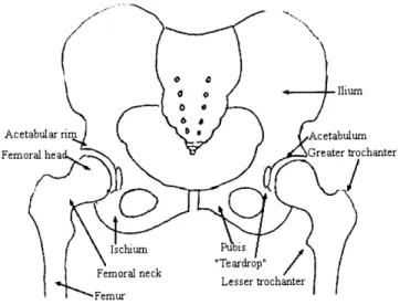
FIGURE 2.1: SCHEMATIC DIAGRAM OF BONY ANATOMY IN THE PELVIS ... 11

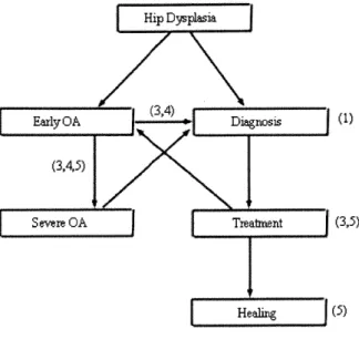
FIGURE 1.1 FLOW CHART OF OA PROGRESSION AND TREATMENT, WITH THE THESIS CHAPTER INVOLVEMENT IN PA R E N T H E SIS . ... ... ---. ---.-.- ... ... 15... 15

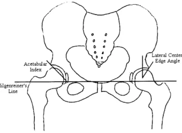
FIGURE 2.2: SCHEMATIC DIAGRAM OF THE FULL PELVIS DESCRIBING RADIOGRAPHIC PARAMETERS USED IN THE DIAGNOSIS OF HIP DYSPLASIA. ... 18

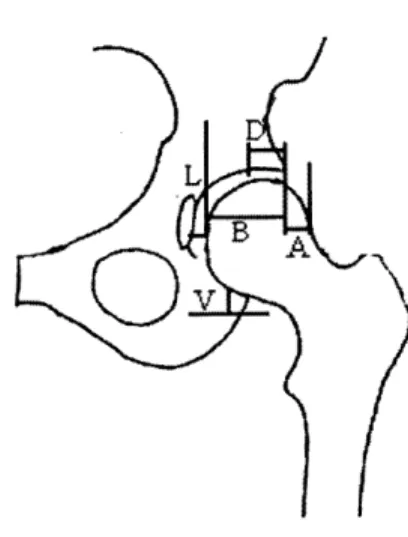
FIGURE 2.3: RADIOGRAPHIC PARAMETERS ON HEMI-PELVIS... 19

TABLE 2.2 RESULTS OF MRI MID-SLICE DIGITIZATION FOR RADIOGRAPHIC PARAMETERS... 23

TABLE 2.2 RESULTS OF THE X-RAY DIGITIZATION FOR 4 PATIENTS AVERAGED OVER 3 TRIALS. ... 24

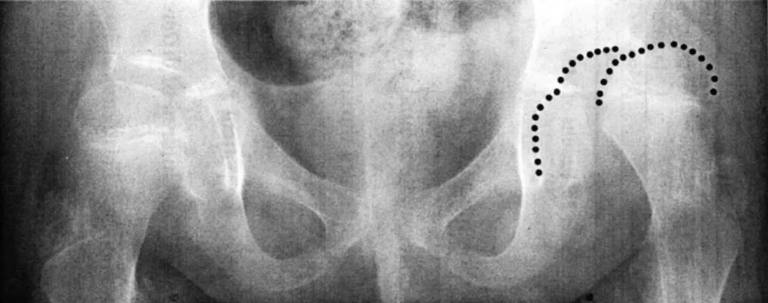
FIGURE 2.4 PLAIN RADIOGRAPH OF PATIENT IA IN NEUTRAL POSITION... 24

TABLE 2.3. TABLE OF THE R2 VALUES FROM THE LINE FIT OF RADIOGRAPHIC PARAMETERS FOR THE 10 HIPS AT N EU TRA L PO SITION . ... 29

FIGURE 4.1: EXPERIMENTAL TEST SETUP FOR THE CALCULATION OF CARTILAGE DISPLACEMENT... 40

FIGURE 4.2. CROSS-SECTIONED JOINT WITH REFLECTIVE TAPE MARKERS LABELED WITH NUMERICAL ASSIGNM ENTS USED IN DATA PROCESSING. ... 41

FIGURE 4.3: DISPLACEMENT (MM) VS. TIME (S) OF THE INSTRON ACTUATOR DURING THE FIRST TEST (2.5 MM; 0 .1 M M /SE C )... ... .. 4 2 FIGURE 4.4: LOAD CELL DATA (N) VS. TIME (S) DURING THE FIRST TEST (2.5 MM; 0.1 MM/SEC) ... 42

FIGURE 4.5: THE FIRST LOADING CYCLE OF THE FIRST TEST (2.5 MM; 0.1 MM/SEC... 43

FIGURE 4.6: LOAD CELL DATA (N) VS. TIME (S) OF THE SECOND EXPERIMENT (1.5 MM DISPLACEMENT; 15 Hz). THE GRAPH ON THE RIGHT REPRESENTS LOAD OVER THE ENTIRE REGIME, WHILE THE GRAPH ON THE RIGHT IS DATA FROM THE LEFT GRAPH 5, 15 AND 25 MINUTES AFTER LOADING BEGAN... 44

FIGURE 4.7 PROPOSED IN VIVO CONTROLLED DISPLACEMENT DEVICE. ... 45

FIGURE 4.8 ORTHOFIX M111 MINI-RAIL FIXATOR WITH CUSTOM MODIFICATIONS ... 46

(9)

FIGURE B. I GRAPHICAL METHODS FOR FINDING THE INSTANTANEOUS CENTER OF ROTATION... 75

FIGURE 3.2 GEOMETRIC RELATIONSHIP FOR GRAPHICALLY MAPPING REULEAUX METHOD... 78

FIGURE B .3 ROTATION OF COORDINATE AXIS ... 80

FIGURE B.4 RIGID BODY M OTION IN A PLANE... 81

FIGURE B.5 OEC M INI6600 DIGITAL M OBILE C-ARM ... 84

FIGURE B.6 RIG USED FOR EXPERIMENTAL TESTING OF CENTER FINDING SYSTEM. ... 85

FIGURE B.7 PLOT OF THE COORDINATES FROM MARKERS 2-5 FROM EACH IMAGING MODALITY THROUGH EACH DEGREE ROTATION (0-20). . ... ...--... ---.---... 87

TABLE B. 1. CENTER OF ROTATION ERRORS FOR DIGITIZED DATA. ... 89

FIGURE C. 1: OUTPUT FOR ACETABULAR RADIUS = 10; FEMORAL HEAD RADIUS = 4; DISTANCE BETWEEN C EN TER S = 6 . ... ... 9 8 FIGURE C.2: OUTPUT FOR ACETABULAR RADIUS = 10; FEMORAL HEAD RADIUS = 8; DISTANCE BETWEEN C EN TER S = 4 . ... .... ...--... 98

FIGURE C.3: USING THE DATA FROM TABLE 2.: OUTPUT FOR ACETABULAR RADIUS = 31.35; FEMORAL HEAD RADIUS = 18.07; DISTANCE BETWEEN CENTERS = 14. ... 99

Cooper, IA., MSME Thesis

9

(10)

CHAPTER

Introduction

1.1 Background

J. Anthony Herring writes, "[Developmental Dysplasia of the hip (DDH)] remains one of the most difficult disorders to understand and treat in all of orthopaedics. Many

pitfalls of management have been identified, and yet an individual patient may not respond to the usual treatment for reasons not understood. [1]." Herring's confusion is well supported throughout the orthopedic community.

What is hip dysplasia? The terminology of the Developmental Dysplasia of the Hip (DDH) is often arbitrary, and the vocabulary can be used haphazardly. DDH is sometimes used synonymously with Congenital Dislocation of the Hip (CDH), while some deem these separate disorders altogether. Similarly, dysplasia, which implies a deficiency in the shape of the acetabulum, is frequently interchanged with dislocation, which describes the location of the femoral in relationship to the acetabulum. The following definition will be used for the purposes of this thesis: DDH is an abnormality of the hip that is characterized

by an instability or dislocation of the femoral head relative to the acetabulum. This

includes dislocation (the complete loss of contact between the femoral head and the acetabulum), subluxation (not total dislocation, but some loss of contact between the

(11)

medial portion of the acetabulum and the femoral head), and geometric anomalies (any incongruency in size or shape between the femoral head and acetabulum). DDH, hip dysplasia, and hip instability are considered the same for the principles in this thesis.

The human hip is characterized as a ball-and-socket joint that permits rotation as well as movement in all spatial planes. Legal [2] refers to the hip joint "an imperfect evolutionary solution to the problem of bipedal gait." He continues to explain that for the proper functioning of any joint, there must be a perfect balance between "the stresses acting on the joint and the ability of the joint to withstand those stresses." When an imbalance is present and is left untreated, hip dysplasia almost certainly leads to osteoarthritis of the hip [8-11]. Untreated hip dysplasia accounts for as much as 76% of all cases of osteoarthritis in the hip [3].

Ilium

Acetabular rm Acetabulum

Femoral hea Greater trochanter

Ischium ius

Femoral neck ".Teardrop"l Lesser trochanter

Femur

Figure 2.1: Schematic diagram of bony anatomy in the pelvis

The prevalence of hip instability appears in I to 21.8 of every 1000 infants born [1, 4,

5]. Clinical symptoms of DDH in walking children may include hip pain, limp, restricted abduction, stiffness, shortening of the thigh and increased lumbar lordosis. When the

11

(12)

disease is diagnosed during early development (before 6-9 months of age), infants are treated with bracing techniques with an 88% - 95.6% success rate [5-7]. In general,

treatment options include closed reduction (using a brace or traction) in infants, open reduction in toddlers, redirectional femoral and acetabular osteotomies in children and young adults, and finally total joint replacement in older patients with established osteoarthritis.

Osteoarthritis (OA) is a degenerative disease of articular cartilage that occurs in 21 million Americans [12]. Biochemical, metabolic, histological and biomechanical changes to the joint cartilage, synovial fluid and subchondral bone are all associated with OA [13]. The exact pathogenesis of OA is unknown but has been induced experimentally by both biochemical and mechanical manipulations [14-16]. If the exact pathogenesis of OA were clear, one could theoretically design an effective treatment. However, because multiple etiologies have been postulated and the regeneration of hyaline cartilage is slow, treatment options are limited and remain empirical.

With tissue engineering alternatives not yet perfected, and arthroplasty failure occurring 10 to 15 years following implantation, one of the best recommended options in younger and active patients with abnormal hip geometry remains surgical intervention. There are many techniques to perform osteotomies in the hip but the premise always remains the same: to optimize the distribution of load by minimizing pressure within the joint and restoring joint "stability." These goals rely on the assumption that mechanical factors are responsible for the development of OA in an untreated joint and the apparent joint healing following a successful surgery. While retrospective analysis of patients by radiographs and clinical exam have demonstrated improvement in hip function, there could

(13)

be other factors involved in the surgical intervention: reducing or increasing the moment arm of the surrounding muscles and ligaments, tightening or loosening the joint capsule, changing the blood supply, etc. Therefore the question remains whether these current surgical goals are correct and are the only factors affecting joint health postoperatively. Specifically, what is the appropriate objective function for surgical intervention that will prevent or ameliorate the development of osteoarthritis?

The development of an objective function, whereby a surgeon could straightforwardly prescribe the appropriate reconstruction technique, could be an important step to better understanding DDH and its role in the development of OA. To experimentally validate this function a method is needed to simulate the mechanical anomalies presented in a dysplastic hip using a simple model that can be subjected to parametric variations.

1.2 Objectives

The objectives of this thesis are threefold:

1) To develop a tool to quantify the severity of DDH using standard radiographic

measurements and to reexamine these measurements in an effort to better describe joint abnormality.

2) To propose a hypothesis for a theoretical objective function for surgical planning of osteotomy

Cooper, JA., MSME Thesis

13

13 Cooper, JA., MSME Thesis

(14)

3) To develop the tools and protocol needed to experimenally derive an objective function

for the surgical planning of osteotomies about the hip, minimizing the occurrence of

OA. To develop a method to validate the legitimacy of the proposed objective function.

1.3 Overview

This thesis presents a set of tools that can be used in several aspects of the diagnosis and treatment of the hip dysplasia. Figure 1.1 diagrams the progression of DDH to OA and the relationship of each chapter of this thesis to these stages of development.

Chapter 2: The current tools used to quantify hip dysplasia and collect quantitative factors used in hip dysplasia include radiologic measurements. A semi-automated tool to calculate a series of radiologic measurements from manually digitized points is presented in this chapter. These measurements represent the current factors used clinically to measure the severity of hip dysplasia. Chapter 2 discusses the downfall of these parameters and suggests the consideration of new parameters for the quantification of DDH.

Chapter 3: A hypothesis for an objective function for surgical planning of osteotomy is presented, along with supportive theory.

Chapter 4: An in situ method for describing cartilage deformation when a mechanical displacement is induced to a joint is offered. This technique will be used for the testing of the theories described in Chapter 2.

Chapter 5: A suggested protocol for the validation of the objective function presented in

Chapter 3 is described, as well as further uses for the system developed in Chapter 4. Appendix B: To carry out the experiments in Chapter 5, a surgical tool for calculating the center of rotation of a joint is needed. The tool described herein can be used real-time in

(15)

the operating room for surgical guidance of metal pins into the center of rotation of a joint. The accuracy and precision of the tool is discussed.

Hip Dysplsi

(3,4,5)

vrSevere OA Treatment (3,5)

Heali ng (5)

Figure 1.1 Flow Chart of OA progression and treatment, with the thesis chapter involvement in parenthesis.

Cooper, l.A., MSME Thesis

15

(16)

CHAPTER

Diagnostic Tool For

Evaluating Developmental

Dysplasia of the Hip

An instability of the hip occurs in as many as 21.8 of every 1000 births [3-5], and left untreated accounts for as much as 76% of all cases of hip joint osteoarthritis [2]. Identification of hip dysplasia is fairly arbitrary since there is not a defined protocol for diagnosis. Recognition of the disease is based upon physical examination and a variety of radiographic parameters. A tool has been developed that can be used to calculate a number of standard two-dimensional measurements used clinically to diagnose and quantify developmental dysplasia of the hip. A redefinition of clinical terms and their associated measurements is proposed that will better quantify the dysplastic hips for diagnosis and aid in treatment decisions.

2.1 Motivation

Standard x-rays are two-dimensional projections of complex three-dimensional anatomy. Physicians and radiologists generally make diagnostic measurements for hip dysplasia via estimation or directly on patients' x-ray film. These parameters describe joint

(17)

shape, coverage, congruency of fit, and stability of the joint. An alternative method for evaluation of parameters that is theoretically more precise, more time efficient, and allows for easier collection and comparison of data from a set of patients, has been developed. A MATLAB based program has been created where the physician can manually digitize plain radiographs to calculate a variety of useful parameters for characterizing hip dysplasia. The shortcomings of these parameters are analyzed and a set of parameters that may better describe the disease is presented.

2.2 Introduction

The diagnosis of hip dysplasia in the children has been accomplished first through the use of physical examination. Newborn hips are maneuvered and palpated in adduction and abduction to dislocate and reduce the joint and classify the instability [5]. Following infancy, limp, leg length differences, and asymmetry in range of motion are used as indicators for the disease. Secondly, imaging modalities are commonly employed. Plain radiographs have been used for decades, while ultrasound, arthrogram, MRI and CT are more current diagnostic tools. Many radiographic parameters have been defined for the diagnosis, classification and evaluation of the severity level of DDH. Since each parameter generally describes only one characteristic of the condition, a few parameters are often used in concert.

Typical radiographic parameters include (but are not limited to): lateral center edge angle, acetabular index of depth to width, femoral head extrusion index, acetabular index, lateral subluxation, superior subluxation, and peak-to-edge distance (Figures 2.2 and 2.3).

(18)

A few of these parameters are based on a reference line drawn through the inferior edge of

the anatomic teardrops (Hilgenreiner's line) (Figure 2.2). Lateral center-edge angle (Wiberg's center edge angle) is the angle formed by drawing a "line from the center of the femoral head to the lateral edge of the acetabular roof and a line drawn superiorly from the center of the femoral head and parallel to the longitudinal axis of the body [14] (Figure 2.2)." Center-edge angle is a measurement of the femoral head-acetabular relationship in the frontal plain, describing the degree of lateral coverage of the femoral head. Acetabular index of depth to width is simply the ratio between the depth and width of the acetabulum. This ratio gives the physician an indication of the sphericity of the weight bearing area. Femoral-head extrusion index is defined as the ratio between the horizontal length of the portion of the femoral head lateral to the edge of the acetabulum to the total horizontal width of the femoral head (in Figure 2.3: A/[A+B] x 100%). Femoral-head extrusion index

0 0

Lateral Center

Acetabular Edge Angle

Index

Hilgenreiner~sN

Figure 2.2: Schematic diagram of the full pelvis describing radiographic parameters used in the diagnosis of hip dysplasia.

(19)

L

K)V

Figure 2.3: Radiographic parameters on hemi-pelvis.

(A/[A+B] x 100% = femoral head extrusion index; L = lateral subluxation; V = superior subluxation; D = peak-to-edge distance.)

is a measurement of the femoral head uncovering - the percent of the femoral head that is not contained within the acetabulum. The acetabular index, which measures the angle of the acetabular roof, (also called acetabular angle or Hilgenreiner's angle) is the angle formed by the intersection of the line from the roof of the acetabulum (the sourcil or weight-bearing zone of the acetabulum) with Hilgenreiner's line (Figure 2.2). Lateral subluxation is the horizontal distance from the lateral edge of the teardrop to the most medial portion of the femoral head (L in Figure 2.3). Superior subluxation is the vertical distance from the inferior acetabular ischium to the most inferior part of the femoral head (V in Figure 2.3). The subluxation measurements quantify the position of the femoral head within the acetabulum. Finally, peak-to-edge distance, a measurement of the acetabular size, is the distance parallel to Hilgenreiner's line from the apex of the acetabulum to the acetabular rim (D in Figure 2.3).

19

(20)

Physicians and radiologists generally make these measurements via estimation or directly on the patients' x-ray film using a wax marker, ruler and protractor. A computer program was developed whereby images can be manually digitized to quantify the two dimensional radiographic parameters listed above. This program is intended for physicians interested in diagnosis and/or quantification of hip dysplasia and researchers interested in comparing imaging modalities or for the tracking of surgical outcomes or disease pathogenesis. It is proposed that this system will provide a more efficient, objective, and precise method for the evaluation of hip dysplasia.

There is a need to quantify DDH for diagnosis, yet the diagnostic limits have not been established and remain unclear. Measurement of parameters is fairly arbitrary and depends upon the judgment, tools, experience, and bias of the observer. Many parameters assume joints should be circular or spherical and have a definite center, when this may not be the case. Repeatability of patient positioning, scaling issues, different imaging modalities and variations of patient size all make individual images difficult to compare. This method is a tool for studying currently accepted parameters, and brings about ideas

for the reconsideration of measurements that have been used for decades.

2.3 Methods

A program was written in MATLAB (The MathWorks, Natick, Massachusetts)

(Appendix A) to read image files and prompt the user to digitize bony joint anatomy. Figure 2.4 shows an example of a patient x-ray with the left acetabulum and femoral head digitized. The program circle fits the acetabulum and femoral head using a least square

(21)

algorithm to calculating the radius, center and root mean square error of the digitized points on the bony surfaces to the calculated circle. The circle is drawn onto the image and the user can verify that the calculation best represents the joint anatomy. If accepted, the user is prompted to digitize additional joint anatomy (anatomic "teardrop," acetabular rim, lateral, proximal and inferior edges of the femur, and acetabular apex and depth). From this information, the following parameters can be calculated: lateral center edge angle, acetabular index of depth to width, femoral head extrusion index, acetabular index, lateral subluxation, superior subluxation, and peak-to-edge distance. All values are printed on the screen and also saved into a text file.

Prior to testing the patient images, the circle fitting function using least squares fitting in MATLAB was tested for varying digitized arc length and input noise level of the digitized points. It was expected that between 25% and 50% segment of a circle was digitized when studying the patient data. Noise was created at 5 levels using random number function to create perturbations of the points of an ideal circle to be fit. This test was performed to verify that slight variation in manual digitization, and segment data will still allow the fitting algorithm to be accurate within acceptable limits.

Also prior to testing, the precision and interobserver repeatability of the program was determined using MRI mid-slice data from two patients used in the x-ray study. The radius of the right and left femur and acetabulum, acetabular index, center edge angle and femoral head extrusion index were measured using the MATLAB algorithms. Each image was measured four times, alternating patients in an attempt to eliminate the observer remembering the previously digitized path, and digitize based only on joint geometry.

cooper, IA., MSME Thesis

21 2 1

(22)

Four patients (3 males and one female), ranging in ages from 4 years 8 months to 8 years 3 months (average 6 years 10 months) undergoing osteotomies for diagnosed severe bilateral hip dysplasia were chosen for this study. X-rays in the neutral and the frog lateral (abduction) positions were included for each patient, one patient's data at two different points in time (five months apart) in the neutral and frog lateral positions were used (for a

total of 10 hips at two positions). Patient X-ray data was scanned using a high-resolution x-ray scanner (Eskoscan 2540, Purup-Eskofot, Inc. Kennesaw, Georgia). One observer performed data collection and the average of 3 repeated measurements was calculated for

each patient and position.

2.4 Results

From the testing of the least squares fitting function, there was no significant change in the curve by changing the number of points to be fit. For small imposed noise levels and arc lengths covering 50% or more of the circle there was no significant change in the expected radius and center results. With no noise, error is on the order of 10-6 for arc length to 25% of the arc and 10% of the degrees (i.e. 9 points) on the arc fitted. With noise level created by altering the y-coordinate by a randomly generated percentage, and 25% of the arc digitized, the error of the fit curve compared to the ideal curve, the error was determined on the order of 10-2. Large noise levels and arc lengths of 25% or less in most cases expectedly proved to have a larger error in calculation of the expected results. From these results, the algorithm has been judged to be accurate for these purposes.

(23)

From the MRI precision study, there was a fairly good precision between femoral radius and the three radiographic parameters measured. The average data are presented in Table 2.2. Standard deviations were 2.8%, 11.2%, 9.9%, and 7.2% of the average for the femoral radius, acetabular index, center edge angle and femoral head extrusion index, respectively. The acetabular radius was not in such agreement between trials. The bony

Femoral Head Radius Acetabular Radius LCEA FHEI Al Patient #3 Left 11.3537275 56.204345 22.6084 89.2109 35.63682

Right 14.28695 49.4254225 10.2807 62.1125 44.4169 Patient #4 Left 9.16556675 36.9714 25.89832 102.7586 35.20241 Right 9.5907667 45.5 56.2869 142.130975 38.559

Table 2.2 Results of MRI mid-slice digitization for radiographic parameters.

femoral head on the MRI images is an easy landmark to define. The acetabulum becomes difficult to differentiate around the medial portion in the MRI images, therefore only a few points could be digitized through this region and the circle fitting become less accurate as

the digitized segment becomes shorter and more of a straight line.

Results of the patient x-ray data are shown in Table 2.2. Though is meaningless to compare anatomy of children of different sexes and ages, the radii results were fairly close over the patient set. The femoral head radius averaged over all of the patients at both positions was 18.07 ± 3.98 mm. The acetabular radius was calculated to be 31.35 ± 7.53

mm for the same population. In general, both femoral and acetabular radius increased with age. Radiographic parameters had fairly good accuracy within the three trials for each patient and position. However, between positions, patients, and opposite hips standard

23

(24)

Patient Age Side Fern Rad (mm) Fern Err Acet Rad(mm) Acet Err LCEA (deg) ADTW FHEI Al (deg) LSUB (mm) SSUB (mm) P2ED (mm) 1 8y3m Left 21.67 0.05 34.69 0.05 55.35 16.87 94.51 64.77 27.32 18.63 9.83 _____ Right 20.87 0.07 32.72 0.03 21.32 7.71 71.79 58.15 23.38 28.06 6.55 7y8m Left 21.07 0.04 31.53 0.05 22.14 13.04 67.93 61.73 19.49 29.94 9.26 Right 20.07 0.04 30.56 0.04 4.58 4.44 38.23 54.71 13.65 29.29 10.03 2 8ylm Left 19.47 0.04 36.09 0.05 10.27 16.31 53.37 61.16 50.58 32.69 8.60 Right 19.21 0.03 35.61 0.13 19.81 9.16 73.09 61.19 18.57 30.42 4.99 3 4y8m Left 15.84 0.09 46.14 0.05 12.62 14.07 46.83 59.03 18.17 26.28 7.97 ________Right 15.86 0.13 33.78 _ 0.05 8.99 6.77 45.05 56.27 19.47 27.58 6.86 4 5y6m Left 11.94 0.07 22.47 0.08 22.06 32.43 81.45 63.02 16.47 24.46 2.87 Right 10.82 0.03 17.38 0.04 57.14 7.65 121.49 74.75 18.89 16.94 3.07 AVERAGE 6ylOm 18.07 0.06 31.35 0.06 19.73 11.28 60.81 59.62 19.76 28.65 8.43 STDEV 3.98 0.03 7.53 0.05 16.74 10.01 25.30 7.69 13.60 7.72 3.92 NORMAL 20-30[14] 33-38[14] 13 [15]

Table 2.2 Results of the x-ray digitization for 4 patients averaged over 3 trials. Where Fem Rad = femoral radius; Fern Err = root mean square error of the circle fitting of the femur; Acet Rad = acetabular radius; Acet Err = root mean square error of the circle fitting of the acetabulum; LCEA =lateral center edge angle; ADTW = acetabular depth to width; FHEI = femoral head extrusion index; Al = acetabular index; LSUB = lateral subluxation; SSUB =

superior subluxation; P2ED = peak-to-edge distance.

Figure 2.4 Plain radiograph of Patient la in neutral position, with the left acetabulum femoral head digitized for curve fitting. Q

(25)

deviations were large.

A comparison of the mid-slice MRI data to the X-ray data for two of the patients

studied showed an average 24% error in the calculation of femoral and acetabular radii, center edge angle, femoral head extrusion index and acetabular index. The difference could be attributed to the difficulty in differentiating structures in the MRI images, human error arising from manual digitization, and error from manual digitization of the x-ray scaling. Also even though x-rays are acceptable for measurement in the clinical community, x-rays are in fact shadow images and may depend upon the radiation beam and the beam source distance from the imaged object (termed the fan beam effect). Standard deviations were lowest in center edge angle and femoral radius (2.82 and 1.78 respectively) and highest in the femoral head extrusion index (17.92) and acetabular index (17.55).

2.5 Discussion

Radiographic differences will naturally occur since the severity of the DDH for each hip may not be identical, not to mention inherent differences in the sex, age and size of patients. The measured values of lateral center edge angle, acetabular index and lateral subluxation for most of the hips in the study do not fit within the normal ranges given in the literature [14, 15] which indicates hip abnormality. To judge the relative "accuracy" of these measurements, a comparison the program generated results with physician measured data via the traditional ruler and protractor method would be needed. The term "accuracy" seems trivial since the measurements of these parameters are highly subject to the bias of the observer. These measurements are used to quantify the severity of DDH and support

25

(26)

the treatment decisions made. However, the terms do little to characterize the abnormality of the joint, and may be redundant or irrelevant. For example, because patient are different size, absolute measures such as lateral subluxation, superior subluxation, and peak-to-edge distance can not be used to compare patient populations and therefore a practical "normal" range cannot be formed. Acetabular index does little to describe the "dysplasticness" of a joint since this measurement merely describes the angle from one side of the weight bearing zone to the other. There is no incorporation of the geometry of the entire acetabulum in acetabular index. Lateral center edge angle and femoral head extrusion index are good measures of the femoral head coverage, however these parameters alone are not indicative of the entire spectrum of maladies encountered with abnormal hip geometry.

One of the biggest downfalls of current radiographic parameters is the two-dimensionalization of a three-dimensional problem. As the presence of MRI and CT machines in hospitals across the world continues to grow, so to does the opportunity for three-dimensional measurements. The quantification of the parameters within a new set of definitions and measurements, incorporating three-dimensional imaging technology, may be used to better assess treatment options and better define the nature of the joint instability. It has been suggested to categorize the joint measurements under the following terminology: congruency, sphericity, stability, contact area, and containment.

Congruency is defined as the relationship between the curve of the lines formed by measuring the distance from the center of the femoral head to the surface of the acetabulum for every angle around the femoral head. Congruency quantifies the lack of mismatch between radii of curvature for the femur and acetabulum. The calculation of congruency can be made in one of two ways when the center point of the femoral head is

(27)

previously defined, or manually prescribed. One possible method would involve first calculating the distance from every previously digitized point on the femoral head and the acetabular bony surfaces to the femoral head center followed by calculating the angle the digitized points create with an arbitrary reference line that intersects the femoral head center. The other method would involve the user digitizing points on the two bony surfaces at a series of determined angles, thereby allowing a direct comparison of the distance and angle between the femoral head and acetabulum (as compared to a curve fit plot in the prior mentioned method). A lack of congruency in the joint would influence contact area and can be a result of a lack of sphericity.

Sphericity is defined as a measure of "how far off' the actual morphology (digitized points) of the acetabulum and femoral head are to a least squares circle or sphere fit. Using least squares fitting techniques, the center and radius of the acetabulum and femoral head can be calculated using user described digitized points. The level of sphericity can then be described by root-mean-square error of points to the "ideal" curve or

by non-linear regression techniques. The root mean square error for the circle fit in the

current study found that the hips included in this study can be circle fit fairly well. Sphericity is expected to be compromised in patients with Perthes' disease, slipped capital femoral epiphysis, epiphyseal dysplasia and advanced OA. Sphericity is an important parameter for an ideal ball and socket joint: as sphericity in both the femoral head and acetabulum increases, so too does the overall joint efficiency.

Stability is defined as the translation of the center of the femoral head from neutral to both abducted and adducted positions with respect to the center of the acetabulum. Stability is calculated using the coordinates of the center of the acetabulum and the femoral

27

(28)

head from the least squares fit calculation for each of three hip position (neutral, abductions and adduction). The center point of the acetabulum is subtracted from the center point of the femur for each position and the magnitude and direction from the resulting femoral head center position of the abduction of adduction as compared to the neutral position center. Stability quantifies how much motion the femoral head undergoes through abduction and adduction, and would seem to be most related to the containment of the joint.

Contact area is defined as the arc length or area for which the femoral head is in contact with the acetabulum. Contact area can be calculated directly from the MRI images, or by determining a standard distance from the bony surfaces that describes contact (perhaps by knowing cartilage thickness) and mathematically calculating whether or not the femoral head and acetabulum are within this distance. Current surgical planing techniques to minimize pressure in the joint optimize the total surface contact area. Total contact area is related to containment and congruency.

Containment can be defined by a series of clinically defined measures previously described from two-dimensional images: lateral center edge angle, acetabular index, femoral head extrusion index, and peak-to-edge distance. Containment is highly related to joint congruency.

The hip joint is most efficient when the acetabular and femoral head geometry are closely matched (congruency). When the joints are congruent the greatest contact area can occur, which distributes the joint loads more evenly over the surface of the joint maintaining better joint health [2, 16]. A mismatch of the radii of curvature could lead to point contact and high pressures in only one portion of the cartilage. From an engineering

(29)

perspective the optimal contact area occurs when joints surfaces are spherical and the femoral head is completely contained within the acetabular cup, leading to the highest level of stability; anatomically the surface of the femoral head is only 50% contained by the acetabulum in the normal hip. The information from this set of measurements is not limited to diagnosis, but can be extended to surgical planning. For example, if both the femoral head and the acetabulum appear spherical, but are not congruent, it would be assumed that there is a size difference within the joint, and the acetabulum may have to be reconstructed to fit the size of the femoral head. Similarly, if the femoral head appears to be spherical, while the acetabulum is not, an osteotomy may have to adjust in the same fashion. However, if both sides of the joint are spherical and congruent, and there is an instability allowing some subluxation, the surgeon may have to redirect the femoral head or acetabulum to increase the containment.

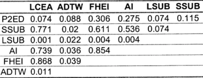
In an attempt to draw relationships between the parameters used to describe hip dysplasia, the average radiographic parameters for each hip in the neutral position of each patient were plotted against each other and fit to a straight line. The R2 values of the line fit are shown in Table 2.3. Lateral center edge angle and femoral head extrusion index correlated the most with the other parameters (average R2 for both is around 0.41), and

LCEA ADTW FHEI Al LSUB SSUB

P2ED 0.074 0.088 0.306 0.275 0.074 0.115 SSUB 0.771 0.02 0.611 0.536 0.074 LS-UB 0.00 1 0.022b0.004 0.004 Al 0.739 0.036 0.854 EHEI 0.868 0.039 ADTW 0.011

Table 2.3. Table of the R2

values from the line fit of radiographic parameters for the 10 hips at neutral position. Where LCEA =lateral center edge angle; ADTW = acetabular depth to width; FHEI = femoral

head extrusion index; Al = acetabular index; LSUB = lateral

subluxation; SSUB = superior subluxation; P2ED = peak-to-edge distance.

29 Cooper, J.A., MSME Thesis

(30)

correlated well together (R2 =0.87). None of the parameters were a good predictor of lateral subluxation (average R2 ₌ _{.029). When radiographic parameters were compared} with the defined parameters of sphericity and stability for the 10 hips, there was no correlation (average R2 ₌_.07).

2.6 Conclusion

A tool that can be used for the quantification of accepted clinical measurements for

the diagnosis of developmental dysplasia of the hip was developed. This tool has been tested with the plain radiographs of 4 patients diagnosed with severe bilateral hip dysplasia and undergoing surgical intervention for the disease. Measured parameters were feasible within the realm of published literature values. It was also suggested to establish a new categorization of terms and measurements used in the diagnosis and measurement of hip instability. These terms may provide an improved insight in the quantification and description of the disease and aid in the recommendation of therapy.

2.7 Future Use

This tool can be used in both a clinical and research setting. Clinically, physicians and radiologists may find this tool useful in the diagnosis of DDH, as well as an outcome measurement following treatment of the disease. Currently this program is being used in research for the radiographic quantification of instability in young adults exhibiting the

(31)

imaging techniques being tested for the diagnosis of early cartilage degeneration. This tool can be used for further comparison of imaging modalities for the diagnosis of hip dysplasia (plain radiographs, ultrasound, arthrogram, computed tomography, and magnetic resonance imaging) and for the correlation of two- and three-dimensional parameters. Furthermore, this tool can assist in the analysis of new measurements that may better aid in the diagnosis of DDH as suggested above.

31

(32)

CHAPTER

Hypothesis for Objective

Functionfor Osteotomy

The relationship of the femoral head to the acetabulum is a fundamental concept in the treatment of hip dysplasia. In Chapter 2 the current two-dimensional parameters used to quantify hip anatomy were examined and new categorization of terms was suggested. A discussion of the current concepts used in planning osteomies and a hypothesis for the re-evaluation of these notions is proposed in this chapter.

3.1 Theory and Hypothesis

Criticism of current radiographic parameters for the quantification of hip dysplasia has developed primarily because of the lack of descriptiveness in the measurements. Additional critique of radiography as a method for characterizing anatomic geometry is the static two-dimensionalization of a dynamic three-dimensional problem. Rab [1] explains that "assessment of the femoral head [in relationship to the acetabulum] by a single anteroposterior roentogenogram of the hip is detrimental to this description because it tends to mislead the orthopedist during a single standing X-ray with the overall function of

(33)

the hip during normal gait and activity levels." Medical imaging, literally, paints a picture of the anatomic problem, and allows physicians to become aware that a problem exists. However, it is proposed here that once a geometric anomaly has been recognized, medical imaging should not be sole provider of information for the surgical planning of to correct this disorder.

The goal of any osteotomy about the hip is to optimize the distribution of load by minimizing the pressure within the joint and restoring joint "stability." This principle relies on the theory that mechanical factors are responsible for the development of osteoarthritis

(OA) in an abnormal joint and that the removal of these factors causes the apparent joint

healing following a successful surgery. The internal stress and pressure distributions within the hip joint have been examined by a number of researchers [2-6]. Surgical planning and guidance tools have been developed to optimize pressure distribution within a joint for surgery [1]. Again, criticism arises from these evaluations.

In situ pressure measurements have been made in a number of ways, including the

introduction of various pressure transducers and miniature piezoresistive transducers to the joint, Fuji Pressensor film, pressure sensitive strips of high resolution matrix-based resistors, and computational modeling. With each of these measurements come weaknesses that reduce the validity of the results. These measurement techniques are extremely invasive and compromise the integrity of the joint. Soft tissues associated with the joint are excised and distorted and joint anatomy is altered with the implantation of sensors into surrounding bone or cartilage or the introduction of a film into the joint space, both of which cause changes in joint mechanical properties, behavior and relationships.

33

(34)

Computational modeling does not compromise the joint, however because of its theoretical nature, requires a validation of the results to be acceptable.

Another difficulty with the characterization of pressure within the joint is the complex nature of cartilage. Cartilage is a complex composite hydrated matrix. The solid components of the matrix are primarily collagen and proteoglycans. Proteoglycans are composed of a core protein with side chains ending in glycoaminoglycan (GAG). GAG chains are negatively charged and provide the matrix with the majority of its fixed charge. The fluid component of cartilage is predominantly water. Nutrients, ions and chondrocytes (cells) can be found in small amounts within cartilage. The collagen matrix appears to provide the tensile support for the material. However, when in compression, the tendency of the negatively charged proteoglycans to repel each other provides the majority of the material properties. When loaded, the speed at which the fluid component of the matrix can flow out of the intricacy of the matrix supplies the time dependent properties of cartilage. The intrinsic complexity of the material makes it difficult for engineers to evaluate both empirically and analytically. Even the characterization of the material in mechanical terms has not been unanimously accepted. Cartilage has been described as biphasic, triphasic, poroelastic and viscoelastic and modeling is often simplified to be linear elastic. Since the nature of cartilage is not yet fully understood, assumptions of minimizing pressure becomes complex at the tissue level.

A change in paradigm is recommended to better tackle the complexity of the in vivo

mechanical environment of a joint from a surgical planning perspective. The movement from a reliance on pressure and stress to the examination of displacements and deformation would provide simpler grounds for measurement. Displacement space can be measured in

(35)

vivo with medical imaging techniques, including Magnetic Resonance Imaging (MRI) and

Computed Tomography (CT). From a modeling perspective, boundary conditions can always be measured in displacement space.

One option for modeling the joint when the positions of joint anatomy are known is through the application of a simple model. Suppose two joint surfaces are modeled as rigid bodies and the initial position of each surface is known. When motion in the system occurs and one rigid body overlaps the other, the assumption is that the amount of overlap of the modeled systems represents the amount of deformation in the actual joint. Because of cartilage material properties compared to those of bone in the joint, the deformation is assumed to be occurring in the cartilage. Presuming models such as this are valid, a shift in purpose can occur in the planning of osteotomy of the hip and a new objective function can be devised.

The hypothesis becomes that the objective function for the surgical planning of osteotomy about the hip is the minimizing of cartilage deformation. A protocol for the validation and testing this hypothesis follow in Chapters 4 and 5. Once the hypothesis has been tested and proved, a surgical planning program can be developed using a simplified model, such as the one above, for the positional recommendation of reconstruction in the joint to optimize cartilage deformation.

Cooper, J.A., MSME Thesis

35

(36)

CHAPTER

Evaluation ofin situ cartilage

deformation

Current methods to test cartilage material properties and cartilage mechanics at a known strain level are carried out by examining cartilage explants. Designing a system whereby a known displacement can be imposed and maintained in vivo would allow researchers to more accurately examine joint health in a physiologic setting. A system has been developed whereby a known displacement can be imposed on an external fixation system that is attached to a sagitally sectioned joint. The actual cartilage displacement is measured and the relationship between the input displacement to the fixator and the measured cartilage displacement is calculated. This relationship can then be used for to impose a known displacement to an in vivo joint.

4.1 Motivation:

It has been shown that mechanical factors play a role in the pathogenesis of osteoarthritis [1-10]. Previous animal studies where osteoarthritis is induced in joints have

(37)

involved the application of external forces. The mechanical conditions at the joint are left unknown or assumed. In order to examine the effects a measurable mechanical parameter (displacement) has directly on cartilage health, a technique must be developed whereby a repeatable known displacement can be applied to cartilage in vivo. This technique can then be applied for the validation of the hypothesis presented in Chapter 3.

4.2 Introduction:

According to the Arthritis Foundation roughly 21 million Americans suffer from osteoarthritis, a degenerative disease of joint articular cartilage that leads to joint stiffness and pain [11]. Articular cartilage is a tissue lining the surfaces of joints and is composed of a low-density collagen matrix and a proteoglycan and protein gel. Because of the complexity of the material, the exact pathogenesis of articular cartilage degradation has yet to be resolved. A number of studies establish that mechanical factors lead to the onslaught of the disease and that mechanical properties of the material are altered as the disease transgresses. For example, an increased strain in the tissue may lead to tissue degradation, similarly, tissue degradation is characterized by a thinning of the cartilage.

Researchers have mechanically induced osteoarthritis experimentally in animal models for decades via injury to the cartilage surface [1], altering of load bearing to a joint though ligament transection or osteotomy [2-6], immobilization [7, 8] and repetitive impulse loading [9, 10]. By and large the previous studies inducing osteoarthritic changes through mechanical means have assumed over-pressurization of the cartilage tissue to be

37

(38)

the dependent variable in the cartilage health. However, current methods for in vivo joint pressure measurements tend to be invasive, inaccurate and relatively unreliable. Alternatively, a change in cartilage thickness is not only a measurable parameter, but can be related to the initiation of degeneration through the relationship of strain to pressure changes.

A majority of work with displacement control has been focused on cartilage

explants with a few studies controlling displacement changes on cadaveric material. The effects of displacement changes on in vivo cartilage health in animal models have been mentioned in joint distraction studies [12] and in limb lengthening work [13]. Because surgical decisions, such as limb lengthening, immobilization, distraction, and osteotomy, tend to change the strain a joint experiences with normal activity, cartilage health can affected. The behavior of the cartilage, the extent to which damage can occur, or healing can be initiated with response to strain changes is an interesting factor to examine from the point of view of osteoarthritis progression.

Previous studies of in situ cartilage deformation have used modem imaging techniques such as computed tomography arthrogram (CT arthrogram), ultrasound, and most recently magnetic resonance imaging (MRI). In comparison to computed tomography

(CT) - the clinical standard of medical imaging techniques, MRI provides the ability to view soft tissues, such as cartilage, and provide some information on tissue chemical composition [14-17]. Though MRI can adequately measure cartilage deformation in static loading cases [18], real time measurement of cartilage deformation is not yet possible with MRI since cartilage response is time dependant and MRI imaging takes time.

(39)

A system has been developed that can be used to impose a displacement on an

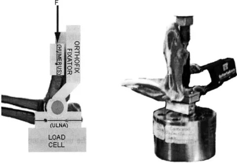
intact joint cartilage in an animal model. By fixing a slightly altered Orthofix Articulated MiniRail Fixator (Figure 4.la) to a rabbit elbow joint, cartilage deformation can be imposed to the joint through surgical pins implanted into the humerus and ulnar olecranon. Because the input displacement may not be completely experienced at the joint cartilage level, a relationship between the in situ cartilage displacement, and an externally measured displacement must be developed. This study validates the use of external fixation and a material testing system to deform cartilage in a cross sectioned animal model joint. An optical tracking system and an extensometer are used to monitor the displacement of the in

situ subchondral bone. Using this system a correlation between the magnitude of cartilage

displacement observed (from the optical tracking and extensometer data) to the input to the external fixator can be made. Using this relationship, experimental studies can be performed whereby a similar apparatus on an intact joint can be displaced and the cartilage displacement can be calculated.

4.3 Materials & Methods:

Adult New Zealand white rabbits were obtained from a study that is not thought to have orthopedic implications, immediately following sacrifice. The left forearms from humerus to carpals were excised and skinned for testing (humerus, radius, ulna and associated soft tissues). Guide holes were drilled into the humerus and ulna to fit the

39

(40)

Figure 4.1: Experimental test setup for the calculation of cartilage displacement. (A) Schematics of test setup, where F represents the input function from the Instron. (B) Photograph of a rabbit elbow joint fixed in the Instron system with exstensometer attached to the surgical pins.

external fixation device, and the joint was frozen overnight in a -20*C freezer at 900 flexion. The frozen joint was cut in half sagittaly using a vertical band saw and was

allowed to thaw wrapped in 0.9% saline-soaked gauze. A metacarpal external fixator was fixed to the joint using surgical pins (Ml 11 Metacarpal Fixator; DM420 Threaded Wire

70/15 1.6mm; Orthofix, Italy). The external fixation system and joint was rigidly fixed into

an Instron 8115 system and a 2200N-load cell, as shown schematically in Figure 4.1. A uniaxial load was applied through the external fixator system to the pins that had been

inserted in the bone.

An Instron extensometer was fixed to the lower anterior humeral pin and medial ulnar pin at approximately 90* flexion. The fixation to the load cell as well as the extensometer

(41)

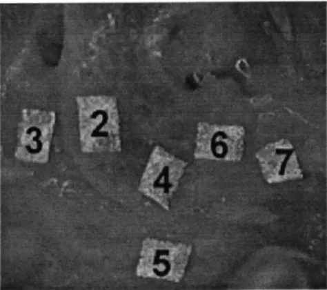
Figure 4.2. Cross-sectioned joint with reflective tape markers labeled with numerical assignments used in data processing.

fixation to the pins is assumed to be rigid. Reflective tape markers approximately 1 mm square (3M) were affixed to the subchondral bone surface (3 markers were placed on the humeral side, and 3 markers on the ulnar side, as pictured in Figure 4.2) and one marker was placed on the Instron actuator. The load cell, actuator, and extensometer were interfaced to PC software to collect data using commercial data collection software (AqcKnowledge, Biopac Inc.), and PCreflex (Qualisys, Inc. Glastonbury, CT) was used to track the reflective markers during testing. Both data collection systems were calibrated independently and prior to testing. Periodically throughout testing, saline was injected into the joint using a 1-cc syringe to keep the joint surface hydrated. During the first test, the joint was cycled for 5 minutes with a trapezoidal loading regime (2.5 mm-displacement

from the initial position, 0.1 mm/sec ramp, 0.008 Hz). In a subsequent test, we cycled the joint to impose a 1.5-mm displacement to the cartilage from the initial starting position at

0.15 Hz with a trapezoidal loading function for 30 minutes. During testing the marker, load

cell, actuator and extensometer data were recorded at 5 data points/second. The test was repeated for 3 joints. The data was imported into Microsoft Excel for data analysis.

(42)

4.4 Results:

Overall, the results for the first test with 2.5-mm imposed displacement with a relatively

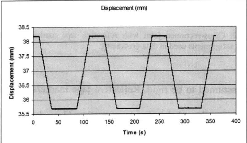
Figure 4.3: Displacement (mm) first test (2.5 mm; 0.1 mm/sec).

vs. Time (s) of the Instron actuator during the

Load cell data (N) vs. Time (s) during the first test (2.5 mm; 0.1

Dspiacement (nn) 38.5 37 36.5 - 36-0 50 100 150 200 250 300 350 400 Time (s) Load (N) 50 50 00 50 200 250 3G0 (350 4''0 -50 z -100 0 -150 -200 -250 -300 Time (s) Figure 4.4: mm/sec).

(43)

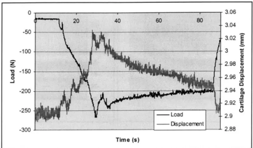
0 3.06 20 40 60 80 3.04 -50 3.02_3.2E -100 3 E z-2.98 -150 0 2.96 -J -200 -294 4 2.92 : -250 -Load 2.9 U -300 Ds placement 2.88 Time (s)

Figure 4.5: The first loading cycle of the first test (2.5 mm; 0.1 mm/sec). The left y -axis represents the load cell data (N), the right y-axis is the difference between reflective markers (4 and 5 from Figure 4.2) on either side of the cartilage surfaces (mm), and the x-axis is time (s).

low strain rate gave expected results. Figure 4.3 represents the displacement regime from the Instron actuator output with time, which shows an accurate portrayal of the intended displacement. The PCReflex and Instron data strongly correlate to each other, as well as the intended displacement. Figure 4.4 represents the load cell data during the test for the same time scale as the displacement data in Figure 4.3. The load is as expected: with an imposed displacement, the cartilage viscoelastic creep properties are exhibited, during the unloading phase, some viscoelastic response is seen, conceivably from soft tissue creep during a lift off phase. A similar response is seen through the PCReflex marker data. Figure 4 shows first displacement cycle load data along with the displacement data for the first cycle of the difference between markers (4 and 5) on opposite sides of the joint. The three curves represent the load response after 5, 15 and 25 minutes of loading. of the subchondral bone surface (assumed to be equal to the cartilage deformation). The load and

Cooper, L.A., MSME Thesis

43 43