Detection of phantom inventories at retail stores using a Bayesian approach

Detection of Phantom Inventories at Retail Stores

Using a Bayesian Approach

by

Sonali Tripathy

Dual degree (B.Tech +M.Tech) in Mechanical Engineering (2010) Indian Institute of Technology Bombay

Submitted to the System Design and Management Program in Partial Fulfillment of the Requirements for the Degree of

Master of Science in Engineering and Management

at the

Massachusetts Institute of Technology

June 2019

C 2019 Sonali Tripathy All rights reserved

The author hereby grants to MIT permission to reproduce and to distribute publicly paper and electronic copies of this thesis document in whole or in part in any medium now known or hereafter created.

Signature redacted

Signature of Author

Sonali Tripathy

System Design and Management Program

7

May 20, 2019

Signature redacted

Certified by

Chris Caplice Thesis Supervisor Executive Director, Center for Transportation & Logistics

Signature redacted

Certified by

Sergio Caballero Thesis Supervisor Research Scientist, Center for Transportation & Logistics

Signature redacted

Accepted by

/

Joan Rubin

MASSACHUSETTS INSTITUTE Executive Director, System Dsign & Management Program OF TECHNOLOGY

THIS PAGE HAS BEEN INTENTIONALLY LEFT BLANK

Detection of Phantom Inventories at Retail Stores Using a

Bayesian Approach

by

Sonali Tripathy

Submitted to the System Design & Management Program on May 20, 2019 in Partial fulfillment of the requirements for the Degree of Master of Science in Engineering and Management.

ABSTRACT

Phantom inventories result from mismatch in the inventory that is actually available at a store on the shelf and the existing inventory as per the data record at any retail store. Inventory on hand (IOH) record for each SKU(stock keeping unit) at any store is summation of on-shelf and back room inventory. Mismatch in this data impacts the product availability at a store

and in turn results in lost opportunities of revenues for the store and the CPG (consumer

product goods) manufacturer. A phantom inventory remains unnoticed unless an intervention such as regular shelf re-stocking, physical audit or consumer enquiry occurs at the store. However, even these interventions may not coincide with actual shelf stock out event and hence, the phantom inventory would continue to exist. This report proposes a Bayesian approach based on consecutive zero sales in the POS (point of sales system) while inventory

IOH remains positive through the observation time. The daily demand is designed using a

negative binomial distribution, which is used further to determine the posterior probability of phantom inventories given a specific set of consecutive days without sales of a SKU at a store. The prevalence of phantom inventories is then calculated using all the number of consecutive days without sales for each SKU store combination and is compared to a Gumbel distribution. This approach has been applied on one data set including POS and IOH data provided by a

CPG manufacturer, where the prevalence was found to be 11.63%.

Thesis Supervisors:

Chris Caplice, Executive Director at MIT Center for Transportation & Logistics Sergio Caballero, Research Scientist at MIT Center for Transportation & Logistics

THIS PAGE HAS BEEN INTENTIONALLY LEFT BLANK

ACKNOWLEDGEMENTS

I would like to deeply thank my thesis advisors Dr. Chris Caplice, Executive Director and Dr. Sergio Caballero, Research Scientist at the Center for Transportation & Logistics (CTL) at MIT for this opportunity of research. They have been constant source of support and inspiration. They have helped me learn and develop continuously and have always steered me in the right direction when approached with challenge.

I would also like to thank Dr. Francisco Jauffred, Research Scientist at the Center for Transportation & Logistics at MIT. His expert advice has proved instrumental in helping me deep dive into the problem and acquire a holistic approach towards resolution.

I would also like to acknowledge the entire team at the CPG company, who not only provided us with the relevant data but also helped us validate the solutions by sharing their valuable feedback and steering discussions around plausible explanations for produced results.

THIS PAGE HAS BEEN INTENTIONALLY LEFT BLANK

Table of Contents

ABSTRACT

...

3

ACKNOW LEDGEM ENTS...

5

TABLE OF FIGURES

...

9

CHAPTER 1

- PROBLEM

DESCRIPTION

...

11

CHAPTER 2 - LITERATURE SURVEY

...

13

2.1 HIDDEN MARKOV MODEL ... 13

2.2 ZERO SALES MODEL

...

16

2.3 CLASSIFICATION METHODS...

17

2.4 COMPARATIVE STUDY OF ALGORITHMS... 20

CHAPTER 3 - METHODOLOGY...

22

CHAPTER 4 - IM PLEM ENTATION

...

27

CHAPTER 5 - CONCLUSION

AND

FUTURE RESEARCH

...

34

THIS PAGE HAS BEEN LEFT BLANK INTENTIONALLY

Table of Figures

Figure 4.1: Inventory on hand vs sales data comparison

...

27

Figure 4.2: Average days with sales per week... 28

Figure 4.3: Average days with sales per week for weekdays...29

Figure 4.4: Average days with sales per week for weekends

...

29

Figure 4.5: Comparison of weekday and weekend rates per day...30

THIS PAGE HAS BEEN LEFT BLANK INTENTIONALLY

Chapter 1 - Problem Description

A retail store is the last stop for any supply chain management process and it is crucial to ensure

error free store execution for the end customers. The store execution involves maintaining shelf availability, managing the backroom stock and seamless movement of material from the backroom to shelves in the store to ensure availability of products to end customers. This makes the store executions challenging as some SKUs would be fast moving over others, making the cycle of shelf-replenishment different for different SKUs. This cycle would also change over season, as the demand of the product would vary over time. Moreover, the Inventory on hand (IOH) data only keeps track of overall inventory in the store, which is the sum of backroom inventory and on the shelf inventory. There is no way to identify shelf out of stock conditions from the IOH inventory data as well. The IOH data itself could be error prone due to improper scan or store theft.

Shelf out of stock (OOS) instances result in missed revenue opportunities. In case of promotions, an item might be bought in bulk by the customers, resulting in quicker shelf OOS than in normal situations. Unpredictability in the shelf-OOS situations turns into a huge challenge, with a huge impact on lost revenue opportunities. Some stores indulge in shelf-audits to cater to this challenge. However, the audit frequency itself would have an impact on the ability to detect any shelf-OOS or altogether elimination of occurrence of such instances. Also, the shelf-audits cost might exceed the loss in sales opportunity over a duration. Hence, this portrays an optimization problem with respect to cost of audits and loss in sales revenue.

Phantom inventory is defined as an instance when an inventory record system reports the availability of a certain SKU, while in reality it is unavailable on the store shelf. Such an instance

could be caused due to theft of items, error in data entry, deliberate fraud or improper barcode scan.

This report summarizes an approach that utilizes a predictive model to detect phantom inventory. This model utilizes the data gathered from POS system - both transaction and inventory record details for each SKU in a particular store. This model could help predict an instance of phantom inventory by analyzing the new transaction data and inventory record in the store systems. This report also puts across methodologies that has been explored by other research groups and summarizes the model that was developed by MIT CTL (MIT Center for Transportation and Logistics) research group.

Chapter 2 - Literature Survey

On shelf OOS research has been an ongoing research for a decade. On shelf OOS has a direct relationship with inaccurate inventory managed by stores. This section summarizes the research around mechanisms used to detect shelf OOS instances by utilizing the POS data and audit data from stores for various SKUs.

2.1 Hidden Markov Model

Montoya and Gonzalez (2019) propose a hidden Markov model (HMM) [1] to identify on-shelf

OOS instance through detection of changes in sales patterns as a result of unobserved states of the

shelf. The approach was validated against visual inspection data of on-shelf stock. The model resulted in detection power of 63.48% and false alerts of 15.52%. The power of detection was highest for medium incidence products at 77.42% and the false alarm rates was lowest for low-incidence products at 7.32%.

Inventory data was not used to develop this methodology as it is deemed ineffective for OOS detection, since the number of units of any SKU in the inventory is the sum of inventory on shelf and in the backroom, and this number cannot be directly correlated to the number of units of the

SKU on shelf. Only POS data was utilized to develop this model. The data was gathered for 70,000

SKUs of 14 products in 10 stores over 15 months. The data was aggregated for over each day -number of transactions that involve product i at store

j

and day t (nijt) and total number of transactions at store

j

and day t (Njt). Incidence data (no. of transactions) was used to create the model instead of the sales data (no. of units purchased in each transaction), as the intent of the model was to ensure on-shelf product availability.

For each product i at store

j,

a probability Usij was assigned, that denotes the probability of the demand is initially in state 's'. One could assume equal initial state probabilities for all states. The transition matrix Qijt denotes the transitions among the states after the first period, If Xijt

E f 1,...,S}denote the demand state of product i at store

j

at time t, then each element of the demand

matrix could be defined as

qijt = P(Xijt = sIXijt.1 = s',priceijt) (2.1)

where qs' > 0 Z 1 qjs's = 1, priceijt is the price of the product i at store j at time t.

The inclusion of price in the model helps capture the transition patterns resulting from any deviation from the regular price. The transition probabilities are defined as

Tr~j'-pq.pricej

S1 = 1+e'1 ceit _(2.2)

i+e-si t

.j S-pipriceijt

e

Tq -Pq-pricery

q2 e I) -JL el p ₁ rcEj ₁t ( 2.3)

1jt= 1+e rJ pSpicei2 t - 1+e p.pricet .

where {Tf',s _{1,..,S} are the thresholds that represent the areas of switching and capture}

regular transition patterns and p- captures the effect of price on transition from state s to any other state. Assuming nijt follows a binomial distribution,

Pijts (nijt

IXijt

= s, zijt) = N t )j(l _ p.ts)Njtnijt (2.4)

To capture the various levels of the demand, the team modeled the incidence conditional probability as in the equation 2.5 below.

Pijts = - (2.5)

where aijs corresponds to the probability that a customer makes a transaction including product i, at store

j

at time t, if the conditional demand is in state 's'. zijt includes all covariates that affect the demand, such as day of the week, price, month, season.

In this model the hidden states represent different levels of partially observable demand. In this case a state s=O was assigned to a state of OOS instance, as an OOS is expected to have a huge impact on product's sales, resulting in substantial decrease in the number of sales.

For a sequence of T daily tickets (niji, nij2, ... , nijT), the likelihood function for product i in all J stores is given by equation 2.6.

L =Hl 1 w' Mij1

Ht=

2 QiLtMijt I (2.6)

where I is a S X 1 matrix of ones. The underlying assumption in this model for parameters estimation is that each product is quite different from the rest of the products. Hence, all the HMM parameters are estimated for each product at store level by using a hierarchical Bayesian Markov Chain Monte Carlo (MCMC).

After each new sales observation, the state of the demand is inferred for product i at store

j

at each time t using the probability of the demand being in state s as given by equation 2.7.

P(Xijt = sn .nit = m.Mi.1

H=

2 Qi jMjW / Lijt (2.7)

The equation 2.7 is used to predict the state the product is at each period of time. The state of maximum probability is assigned as the state of demand. An alert would be generated from the model when the state detected is that of OOS.

2.2 Zero Sales Model

Howard Hao-Chun Chuang [3] [2] proposes another methodology for detection of shelf OOS instances from POS data that screens for consecutive zeros in the sales observations of a specific

SKU [2]. The proposed model also considered factors such as cost, stochastic transition from non-OOS to non-OOS, zero sale probability of underlying demand, manager's perceived non-OOS likelihood,

and random fixes of shelf-OOS on optimal decisions.

z is defined as the number of consecutive periods of zero sales. However, since it is not an accurate representation of the demand due to unobserved shelf-OOS or non-shelf OOS. The demand was assumed to be Poisson or negative binomial. Hence, the underlying demand of a SKU in a period could be considered as a Bernoulli trial with a probability p of zero sale. The state transition matrix across z periods is given by table 1.

State Shelf OOS Non shelf OGS

Shelf OOS 71 0

Non shelf OOS w -W

Table 1: State transition matrix

The parameter w is used to characterize the transition from OOS to no-OOS. This results in a two state Markov chain. The level of w could be used to adjust the perceived risks of shelf-OOS instances.

It is derived that the likelihood of an OOS conditioning on z consecutive zero sales, P(OOSIz) is given by

P(OOS)w1 [(1zp)W(2

P(OOSIz) = ,_,_,3, 2 i-(i-w)p (2.8)

P(OOS)w _(1P) +(-P(OOS))(-W)zz

Under a discrete i.i.d. demand process, the expected number of shelf OOS periods for a specific

SKU at a store, when consecutive z zero sales were observed is given by (derived in the referred

article)

p(w-1) z _(2.9)

1+p(w-1) (p--PWz_

Having derived the equations 2.7 and 2.8, z*, the number of consecutive zeroes a store manager could tolerate before an audit trigger is given by

z* = min {s E(1,2.):k M. P(OOSs). (w1)- s (2.10)

where s is re-shelving inventory level, S is targeted shelf inventory level, k is cost per audit, and M is expected per period margin. Equation 2.8 would be used for P(OOSfs) calculation of z* in equation 2.10.

2.3 Classification methods

D. Papakiriakopoulos [3] studied various classification algorithms to detect shelf OOS instances.

He used POS, replenishment orders, 2 -week spanning promotional plans and daily audit data from 6 different stores of a retail chain. For the audit data, a researcher visited the store at the same hour every day to capture missing products on the shelves for 18 working days.

There were multiple erroneous data points identified in the data sets collected and were eliminated as part of the data cleaning process. These erroneous data points are insightful and summarize some of the contributing factors for unpredictability in the out of stock events or product unavailability. The table 2 summarizes the problems identified.

Data set type Problem Source Data cleaning task

POS data Negative sales value Product returns by consumers Deletion of such records Sales with non-existent code Manually entered product code Deletion of such records Unexpectedly high sales Intra-delivery order between Deletion of such records

quantity two stores

Products ordered by store that Changes in delivery channel Update replenishment

Orders data are not delivered from central mode

warehouse

Multiple same order for Backordering Delete multiple orders consecutive days

Deliveries data Delivered product not New product that retail chain Update of order file with requested by store wants to merchandize delivered products Product assortment De-listed products Product assortment not Remove from product

updated assortment file

Table 2: Data source and problems identified

After the cleaning of the dataset, the data was built for implementing classification algorithms. The last date of transaction of a specific product in a store was identified using the POS data and was labeled as 'OOS' from this date until the date the product was reported as OOS after physical audit. Similar procedure was used to label transaction dates with 'Exists'. These additions expanded the initial POS data set into a medium sized data set. A large data set was created by including products found in product assortment but not in the POS data. These products could be potential delisted products. All these 3 datasets were utilized for training and testing of various classification algorithms. There were several sales features, product features, inventory features and product category features were used in these classification algorithms. These features were selected based on business intuition and data availability. The most relevant features were found to be the ones related to sales, such as items sold for a specific day and the average number of days a product hasn't sold a single unit. The weakest feature was found to be the seasonality factor of product categories. Such factors were removed from the data set.

The next step was to leverage these features in the classification algorithms. 16 different classification algorithms were assessed that could be categorized into statistical, decision tree, rule, neural network and support vector machine. Each classification algorithm was evaluated using the

3 different datasets through a 10-fold cross-validation process. Based on the empirical results from measuring area under ROC curve (AUC), random forest was found to be the best performing algorithm. However, the specificity value for random forest was close to average of all other algorithms. Statistical algorithms such as Naive Bayes and Bayes Net would prove promising in detection of missing product on the shelf due to their high specificity and sensitivity values.

Physical store audits were used for validation of the results from these classification algorithms. Three of the stores had been used for the initial dataset and the remaining three stores signified were control data. Each day after the prediction was made, physical audit helped record the actual missing products. The two measures that were used to determine and assess the capabilities of the system:

Accuracy - how many times the system detects correctly the OOS case

Support - how many examples the system detects correctly an OOS out of all available OOS in the store

The average accuracy of the system was found to be close to 80% and the average support rate was close to 20%. The low support rate could be attributed to the fact that not all aspects of the problem were being assessed in the research.

2.4 Comparative study of algorithms

After keen exploration of all the existing methodologies, it could be established that research groups have explored various statistical models in the past to solve the challenge of timely detection of shelf OOS instances. The majority of the research groups have focused on approaches such as zero sales, binomial, hidden Markov and statistical process control model. Montoya and Gonzalez [1] benchmarked these models by implementing these models on their dataset. The dataset was distributed into three groups - low, high and medium based on incidence rates of shelf

OOS. The high group contained four products with an incidence rate higher than 0.6%. The

medium group had five products with an incidence rate between 0.3-0.6%. The low incidence group had five products with an incidence rate lower than 0.3%. The benchmark models were executed as explained below:

Zero-heuristic: A simple decision rule was used based on the assumption that zero sales in the POS data are caused on by shelf-OOS. An alarm was triggered if there were zero sales of a product in the store during a day.

Binomial model: A binomial distribution was used to characterize the number of transactions containing a certain product. An alarm was triggered when the observed number of sales corresponded to a low probability event (Two thresholds were utilized to signify low probability

event - 0.01 and 0.05)

Binomial zero-sales (BZS): Same approach was utilized as by Chuang et al. [2]. A binomial model was used to estimate the probability of observing zero sales in Z consecutive days. An alarm was triggered if the probability was lower than the threshold for the Z consecutive days. For the benchmarking, Z=1,2 days and threshold of 0.01, 0.05 were used.

Three performance metrics were used for the benchmark comparison- Type I error, false arms and power of detection. The zero sales approach, despite its simplicity had a high power of detection

(54.78%). However, the number of false alarms is equally high (37%), deeming the model

unreliable. The binomial model has the highest false alarm rate (75%). The BZS model performs better with lower false alarms and type I error. Although, the power of detection is lower than best performing models. BZS has better performance for a threshold value of 5% and Z=2 days. The Markov model dominates all other models in regard to power of detection (70%). The type I errors and false alarms are higher than the BZS model, but still comparable in order to be a potentially good model for estimation.

In conclusion, there is still amplitude of opportunity available for improvement in existing models. Further research could be done to determine the impact of product or SKU correlations, promotions or inter-store correlations. Also, if any factors contributing to the higher false alarms or errors could be determined, it could help further enhance the detection power while not compromising on false instances detected. Also, these models could help determine an optimal shelf audit frequency based on the power of detection and false alarm rates of the model being used. It is also essential that models are simplified and data inputs minimized to be able to efficiently manage data cleaning and modeling in future versions.

The next section discusses a mechanism developed by one of the teams at MIT CTL in collaboration with a leading CPG company, that could be implemented at various store locations to identify shelf OOS instances on daily basis. This would help stores better manage the back room and on-the-shelf inventory while minimizing the revenue loss due to lost sales opportunities caused

Chapter 3 - Methodology

As discussed in previous chapters, a phantom inventory is a retail stockout event caused either by an inventory shrinkage or by failure of proper shelf execution. Li Chen [4] proposes two partially observable Markov decision models to cater to these two aspects of phantom inventory. One of the models deals with the shrinkage issue, in which case the actual inventory level is unknown until a store inspection is performed. The second model caters to the shelf OOS problem, in which case an optimal inspection threshold could be determined based the consecutive zero sales period method. These two models along with all the approaches discussed in Chapter 2 are unable to cater to factors such as promotions, seasonal variation in demand of a SKU, different sales rates over weekdays & weekends or implementation of audit at an optimized frequency.

The current ongoing research at MIT CTL intends to address these challenges. The research so far uses a Bayesian approach by identifying consecutive zero sales to detect phantom inventories. The idea behind the consecutive zero sales is to identify consecutive days with zero sales that are unlikely to be observed based on prior demand data.

Due to existing errors in the POS data, owing to phantom inventories and shelf OOS, the sales of a specific SKU as observed in the POS data would not be the accurate representation of demand. To overcome this challenge, we aggregated the number of transactions over the range of available data each day. Further, we assumed the average of all these daily transactions (X) over the range of data as the daily arrival rate of customers. This is a reasonable assumption, given that the data is aggregated at daily level. Assuming C is the expected number of a specific SKU item to be bought by a customer. The expected number of a specific SKU item sold per day (XC) at a store would be given by equation 3.1.

E[S] = kC (3.1) The number of items sold per day could be best modeled using a Negative Binomial distribution

as f(x) in equation 3.2.

f

() -

_r(x+1)r(r)

r(x+r) (1 _ (5rx (3.2)

where r, 6 represent the parameters of the distribution and x represents the daily sales rate. f(x)

defines the probability of sales rate being x, given the parameters r, 8.

The log-likelihood function could is given by equation 3.3.

L (r, 6) = E' In 17(xi + r) - In r(xi + 1) - In r(r) + r In(1 - 6) + xi In 6 ( 3.3)

The parameters could be estimated by maximizing the log-likelihood function.

A = -r ln (1 -S) (3.4)

C = - -6 (3.5)

It is safe to assume that the daily demand of a specific SKU in a store would be independent of demand on any other day, but could be dependent on promotional offers, holidays, weekend or weekdays. Let us define ft(x) as the probability of demand of x items on a day t, St as the sales on the day t and It as the inventory on hand of a specific SKU item in the same store. If an observation is being made for T days for this item at the store, then the inventory is phantom based on the zero sales Bayesian criteria if

P(St = 0, t = 0, 1,.. TjIt = 0, t = 0, 1,.. T) = 1 ( 3.6)

Let p be the prior probability of phantom inventory of a specific SKU in a store. The posterior probability of phantom inventory for a block of days from 0 to T becomes

P(PhantomT) = p (3.8)

p+(1-p) 11T- 1ft(0)

Assuming that the demand probabilities of a specific SKU store combination is constant over the observation period, then equation 3.8 could be rewritten as

P(PhantomT) = 1+e -aT-b (3.9)

where a = -In fo(0) and b = -ln(-)

P

These parameters could be estimated for specific store and SKU combinations by using audit data to create labels for phantom inventories in the data. Once the parameters are estimated, the probability of phantom inventory for a specific day could be found using equation 3.9.

Finally, to use this posterior probability for decision making, a threshold value (x) could be used to identify the instance of phantom inventory. If the posterior probability is greater than cc, then the instance would generate an alert for probable phantom inventory. The condition reduces to equation 3.10.

aT > In - b (3.10)

The value of threshold is a service parameter and depends on to what level risk is acceptable by the store and hence, is a tradeoff between lost sales and cost of physical inspection. It could vary for various SKU and store combinations as well.

The model could be extended for parameters such as weekdays, weekends and promotions by using a linear combination of such parameters as below

alTweekdays + a2Tweekends + a3Tpromotions > In " - b (3.11)

where a, = -In fweekdays(O), where a2 = -In fweekends(O), a3 = -In fpromotions(O) and b =

- ln(~1-). Here the subscripts weekdays, weekends and promotions refers to specific probabilities

p

or parameters related to these variables. Again, all these parameters could be estimated in case of well-maintained audit data and any further variables could be integrated.

The prior probability of phantom inventories that determines the constant term in equation 3.9,

3.10 and 3.11 could be estimated indirectly using probability theory. It is clear that a sequence of

days without sales does not necessarily arise due to phantom inventory. Let z be the probability of zero sales of a SKU in a store on any day. Then if an observation is made for a sequence of T days, the probability of x of these days having zero sales is

p(x) = In (1/z)zx"e-zx- (3.12)

where

in T(1-z) in (1/z)

The equation 3.12 is a Gumbel distribution and the parameter P depends on the number of days in the observation. t could be interpreted as the maximum number of days that would have zero sales when an observation is being made for consecutive T days due to randomness in customer arrivals. It could also be observed from the equation 3.13 that this parameter depends on T.

The probability z of arrival of a customer could be expressed as z = e- for any store-SKU combination where X is the parameter for the distribution. A Poisson distribution is the most popular when modelling the number of times an event occurs in a specific interval of time. This

p(x) = exp (-eu(x)) where

u(x) = Ax - In n(1 - eA) (3.15)

If the largest sequence of days without sales for a store-SKU combination could be attributed to

only chance, then the equations 3.14 and 3.15 would produce uniform distribution over the whole range of period. If however, there is a huge deviation from a uniform distribution, then the probability values from equation 3.14 that are close to 1 are more likely to be produced by phantom inventories in the data set. The prevalence value or the prior probability p as discussed in chapter 2 could be calculated by creating bins from the values produced from equation 3.14 in the interval

[0,1]. p can be then defined as

(no.of observations in the last bin)-(average no.of observations per bin)

(3.16)

total no.of observations

The value of p could vary to some extent depending on the number of bins created to calculate the prevalence value. It would be a good rule of thumb to create enough number of bins to cover the whole sample, while not creating any empty bins.

26

Chapter 4 - Implementation

This chapter focuses on the implementation of the methodology discussed in chapter 3 on data

gathered from various stores of multiple SKUs of products provided by a leading CPG company.

The data made available to team had POS, inventory on-hand inventory, on-order inventory and

in-transit inventory data for a duration of 246 days. A total of 261 SKUs and 176 stores were

included in the data. Based on the data, total of

39953

unique store SKU combinations were

detected as opposed to a possible

45936

combinations. This reflects that not all SKUs were present

at each store. The SKU store combinations with lesser than 246 days of data were eliminated from

the data set. These SKUs may have been discontinued from the store or discontinued by the

company and would no longer be of interest in this analysis.

An initial analysis of the data showed signs of phantom inventories. One such example could be

seen in the figure 4.1. In the highlighted area, there is a significant hike in the inventory on hand

(IOH) level. However, the POS data shows zero sales for over 2 weeks. The POS data before and

after this highlighted period do not have zero sales for an extended period of time. It could be

inferred from this data that there are potential phantom inventories in this dataset.

12

10

6 4

Mar3 Mar 18 Apr 2 Apr 17 May 2 May 17 Jun I Jun 16 JIA I Jul 16 Jul 31 Aug 10 Aug 30 Sep 14 Sep 29 Oct 14 Oct2 No 13

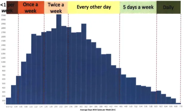
To assess the rate of sales of a specific SKU at a store, the data was aggregated over each week to

calculate the number of sale transactions per week. For each day if sales occurred for a specific

SKU at a store, the transaction value was assigned to be one, irrespective of amount of that SKU

item sold that day at the store. These transaction values were added for each week and this value

was averaged over all the weeks of the data. This average days with sales per week were plotted

in a histogram for all SKU store combinations. The distribution is shown in the figure 4.2. The

majority of SKU store combinations have an average of 1-2 days with sales per week.

<1

Once a

Twice a

Everyother day

5daysa week

week

week

2103 2000 1900 1700 1600 1500 1400 1300 1200 1100 S10DO 800 700 600 Soo 400 300 P, a e 2 2 2 6 2 2 3 e a 3 4 4 4 4 46 8 0 S.2 S 4 S,6 5.8 6.0 62 6.4 6.6 6.8 7.O 7.2 Average Days With Sales per Week (bin)

Figure 4.2: Average days with sales per week

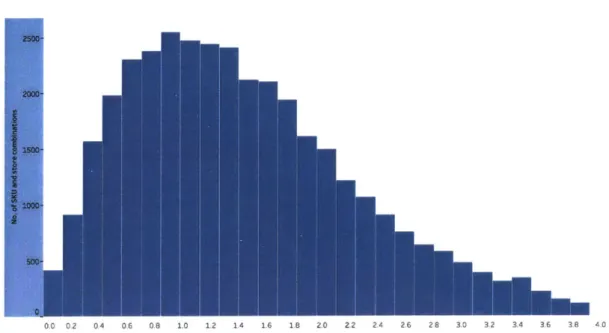
These quantities could significantly vary if the averages were calculated for weekdays and weekends separately. As per the industry team, it was a viable assumption to consider Fridays as one of the weekends in these calculations. Hence there were 4 days of weekdays and 3 days of weekends in each week. The data was now separated for weekdays and weekends and the

aggregation was done separately over weekdays and weekends.

0.0 0.2 0.4 0.6 0,8 1.0 1.2 1.4 1.6 1.8 2.0 2.2 2-4 2.6 28 3.0 3.2 3.4 3.6 3.8 4-0

Avg Days With SDS (bin)

Figure 4.3: Average days with sales per week for weekdays

2500- 2000-2= 1000-

500-0E

.2 C4 I 26 1C 12 12 16 1 20 22 21 26 26 8 0 3.2

Avg Days With Sales (bin)

Figure 4.4: Average days with sales per week for weekends

The average days with sales per week over all the weeks in the data set has an average of

1.44(Mon-Thu) days per week for weekdays and an average of 1.38(Fri-Sun) days per week for weekends

over the whole data set. These two values look close but considering that the base is 4 vs 3 days

for these averages, there might be a statistical difference in the values. Hence, a statistical analysis

over weekdays and weekends in our analysis. Figure

4.5

shows an initial box plot of the data,

where there seems to be a difference in the range of rates and standard deviation in the dataset.

The weekday rates and weekend rates here correspond to average days with sales on weekdays

and average days with sales on weekends divided by number of weekdays and weekends

respectively.

Weekday rates

Weekend rates

41-Mean = 0.3587 Mean = 0.4642

Std. dev - 0.2017 Std. dev 0 0.2272

Figure 4.5: Comparison of weekday and weekend rates per day

Welch T-test was performed on the two data sets of weekday rates and weekend rates to check if

the difference in the datasets was statistically significant. The Welch T-test has different

approaches based on equal or unequal variances of the data sets. The standard deviations are close

to each other. To establish a significant difference in the variances, F-test was performed. (Both

the hypothesis tests

-

Welch and F-test were performed using R coding software and the results

are summarized in this report)

Null hypothesis: Ratio of variances is equal to 1

Alternative hypothesis: Ratio of variances not equal to 1

F-statistic value = 0.78857

Numerator degree of freedom = 35952

Denominator degree of freedom =35952

p-value < 2.2e-16

Alternative hypothesis is true as the p-value is lower than a significance value of 0.05. This implies that there is a significant difference in the variances. The next step was to perform the Welch T-test with unequal variances.

Null hypothesis: Difference in means equal to 0

Alternative hypothesis: Difference in means not equal to 0

t-statistic value = -65.809

Degree of freedom = 70913

p-value < 2.2e-16

Alternative hypothesis true as the p-value is lower than the significance value of 0.05. This helps establish that there is a statistically significant difference in the weekday and weekend rates. This validates the consideration of separate weekday and weekend rates in the model for phantom inventory detection.

As discussed in the chapter 3, based on the Poissonian estimation, the expected demand of a specific SKU at a store on any day could be estimated using the equation 4.1. Here, separate rates

alTweekdays + a2Tweekends > in 1 - b (4.1)

where ai and a2 are estimated based on the negative binomial distribution and b is estimated based on prior probability p as defined in equation 3.15. The threshold value a is an input parameter that the user defines beforehand.

A trigger would be generated by this algorithm if the demand in the observation period of T days

(Et1 At) exceeds the threshold value of cc, while the sales of this SKU remains zero over all these

consecutive days in the store. The continuous steps in algorithm could be explained using the figure 4.6. Start of algorithm Accumulator value = 0 No 'IOH > 0? Yes No

Carry over the

A

value Sales = 0?

Yes

A += Expected Daily demn

NoYs

Figure 4.6: Algorithm flowchart for phantom inventory detection

The prevalence or prior probabilities of the phantom inventories was found to be 11.63% in this data set. The prevalence was calculated as discussed above in chapter 3. Python software was used

to calculate the expected events per bin and events in the last bin, which was later used to estimate the value of prevalence of phantom inventories. This value could be validated by either previously established prevalence values or any audit data that could help estimate prevalence for a specific time period.

Chapter 5 - Conclusion and Future Research

The problem in discussion is undoubtedly complex. The results obtained and insights gained through the research so far is definitely of value to the CPG manufacturer. The use of the methodology developed in this research on the dataset provided by the CPG manufacturer is able to detect a number of instances that could be alerted as Phantom inventories. This detection is solely based on the POS and IOH data. However, there is no way to establish if the instance signaled as phantom is actually a phantom inventory. It is hence crucial to validate this model against any physical audit data available over the same period. This would help quantify the true positives and false positives out of all the highlighted instances .

The intent of this algorithm is to alert the store every day of all the SKUs that probabilistically have phantom inventories. Every such alert results in cost incurred due to physical audit of the SKUs. This algorithm should restrict false positives to an extent such that the cost of audit does not exceed the loss of revenue from prospective sales of phantom inventories.

Price of the SKU, product promotions, inventory in transit are some of the additional parameters that could help further increase the specificity in the algorithm by decreasing the false positives and establishing a better optimization between lost revenues and cost of audit personnel visit. The future research in this area using additional data sets would add value to the existing methodology. Montoya and Gonzalez [1] are able to cater to this challenge by including product price in the model and creating a multi-state model.

Once validated through the audit data, this heuristic approach is simplistic and only requires POS and IOH data to determine a phantom inventory with an acceptable accuracy. This solution caters to the problem with already existing data in the store and requires minimal data management.

Bibliography

[1] R. Montoya and C. Gonzalez, "A Hidden Markov Model to Detect On-Shelf Out-of-Stocks

Using Point-of-Sale Data," Manufacturing & Service Operations Management (INFORMS), Vols. 1526-5498, pp. 1-17, 2019.

[2] H. H.-C. Chuang, "Fixing Shelf Out-of-Stock with Signals in Point-of-Sale Data," European Journal of Operations Research, vol. 270, no. 2018, pp. 862-872, 2017.

[3] D. Papakiriakopoulos, "Predict On-Shelf Product Availability in Grocery Retailing With

Classification Methods," Expert Systems with Applications (Elsevier), vol. 39, pp. 4473-4482,

2012.

[4] L. Chen, "Fixing Phantom Stockouts: Optimal Data-Driven Shelf Inspection Policies," http://dx.doi.org/10.2139/ssrn.2689802, 2014.

[5] H. H. Chuang, R. Oliva and S. Liu, "On-Shelf Availability, Retail Performance, and External

Audits: A Field Experiment," Production and Operations Management (POMS), vol. 25, no. 5,

pp. 935-951, 2016.

[6] D. Papakiriakopoulos, K. Pramatari and G. Doukidis, "A decision support system for detecting

products missing from the shelf based on heuristic rules," Decision Support Systems, vol. 46,