Design optimization of thermal paths in spacecraft systems

(1)

by

Kevin Dale Stout

B.S. Aerospace Engineering The University of Texas at Austin (2011)

Submitted to the Department of Aeronautics and Astronautics in partial fulfillment of the requirements for the degree of

Master of Science in Aeronautics and Astronautics at the

MASSACHUSETTS INSTITUTE OF TECHNOLOGY June 2013

This material is declared a work of the U.S. Government and is not subject to copyright protection in the United States.

Author ... Department of Aeronautics and Astronautics

May 16, 2013 Certified by ... Rebecca A. Masterson Research Engineer Thesis Supervisor Certified by ... David W. Miller Professor of Aeronautics and Astronautics Thesis Supervisor Accepted by ...

Eytan H. Modiano Professor of Aeronautics and Astronautics Chair, Graduate Program Committee DISCLAIMER CLAUSE: The views expressed in this article are those of the author and

do not reflect the official policy or position of the United States Air Force, Department of Defense, or the U.S. Government.

(2)

2

Design Optimization of Thermal Paths in Spacecraft Systems

by

Kevin Dale Stout

Submitted to the Department of Aeronautics and Astronautics on May 16, 2013, in partial fulfillment of the

requirements for the degree of

Master of Science in Aeronautics and Astronautics

Abstract

This thesis introduces a thermal design approach to increase thermal control system performance and decrease reliance on system resources, e.g., mass. Thermal design optimization has lagged other subsystems because the thermal subsystem is not thought to significantly drive performance or resource consumption. However, there are factors present in many spacecraft systems that invalidate this assumption. Traditional thermal design methods include point designs where experts make key component selection and sizing decisions. Thermal design optimization literature primarily focuses on optimization of the components in isolation from other parts of the thermal control system, restricting the design space considered.

The collective thermal design optimization process formulates the thermal path design process as an optimization problem where the design variables are updated for each candidate design. Parametric model(s) within the optimizer predict the performance and properties of candidate designs. The thermal path parameterization captures the component interactions with each other, the system, and the space environment, and is critical to preserving the full design space. The optimal design is a thermal path with higher performance and decreased resource consumption compared to traditional thermal design methods.

The REgolith X-ray Imaging Spectrometer (REXIS) payload instrument serves as a case study to demonstrate the collective thermal design optimization process. First, a preliminary thermal control system model of a point design is used to determine the critical thermal path within REXIS: the thermal strap and radiator assembly. The collective thermal design optimization process is implemented on the thermal strap and radiator thermal path. Mass minimization is the objective and the REXIS detector operational temperature is a constraint to the optimization. This approach offers a 37% reduction in mass of the thermal strap and radiator assembly over a component-level optimization method.

Thesis Supervisor: Rebecca A. Masterson Title: Research Engineer

Thesis Supervisor: David W. Miller

Title: Professor of Aeronautics of Astronautics

DISCLAIMER CLAUSE: The views expressed in this article are those of the author and do not reflect the official policy or position of the United States Air Force, Department of Defense, or the U.S. Government.

(3)

3

Acknowledgments

I thank God for His mercy and the strength He has provided me throughout my life. His sovereignty in both the good times and the bad are constant reminders of the gifts I have been given. I would like to thank my wife Andrea for her unending support. She is my best friend and I cannot wait to see what the future has in store for us. I would also like to thank my entire family – especially my parents, Michael Stout and Antoinette Nelson, and my sister Amanda Stout – for their love and encouragement. Without their influence, I never would have found myself on a path to MIT.

Thank you to my advisors Professor David Miller and Dr. Rebecca Masterson for the

opportunity to be a part of the Space Systems Laboratory. Their mentorship has greatly improved my technical skills as a systems engineer. Furthermore, I'd like to thank other MIT faculty/staff and my peers who encouraged and help me work through my SM degree.

I would like to express my sincere gratitude to the United States Air Force for this academic opportunity. The Air Force ROTC Detachment 825 at the University of Texas at Austin taught me responsibility, teamwork, and leadership. I will always consider Det 825, the cadre and cadets, my first Air Force home. Dr. Hans Mark, Col Christopher Bowman (Ret), and Col Jeffrey Staha took a chance on me during my time in Det 825 at the University of Texas at Austin. Their efforts to enable my first assignment at MIT are both humbling and generous. I thank them for their mentorship, support, and guidance.

The summer internships during my undergraduate education in Group 93 at Lincoln Laboratory heavily influenced my graduate school path. I would like to express my appreciation to Zachary Folcik, Dr. Rick Abbot, and Dr. David Chan for the opportunity to work in Group 93 and providing me with motivation to attend MIT as a graduate student.

(4)

4

List of Figures

Figure 1: Dry mass distribution of average earth-orbiting spacecraft [2] ... 11

Figure 2: James Webb Space Telescope [3] and REXIS; examples of cold regime space systems with a higher than average thermal mass fraction ... 12

Figure 3: Relationship of thesis work with prior research ... 14

Figure 4: Hull, et al. [4] radiator shape variation and design optimization ... 16

Figure 5: Muraoka, et al. [11] design optimization of MMP panels ... 17

Figure 6: Vlassov, et al. [13] heat pipe and radiator assembly geometry from for design optimization ... 18

Figure 7: Traditional thermal design process [14] ... 18

Figure 8: Notional illustration of component-level and collective optimization of thermal paths ... 21

Figure 9: Thesis roadmap ... 22

Figure 10: Top view of REXIS on the instrument deck of OSIRIS-REX ... 25

Figure 11: REXIS design overview ... 27

Figure 12: General spacecraft system thermal environment [14] ... 30

Figure 13: 1-D conduction through a homogenous material [18] ... 33

Figure 14: 2-D resistor grid representation of radiator plate ... 36

Figure 15: Resistor connectivity at arbitrary node location (i,j) of radiator ... 37

Figure 16: Sample nodal matrix structure for 2-D radiator with 10 x 100 discretization ... 39

Figure 17: Collective thermal design optimization process... 42

Figure 18: Example 1-D heat conduction problem ... 46

Figure 19: Gradient-based optimization process [24] ... 52

Figure 20: REXIS thermal architecture ... 58

Figure 21: N2 diagram for REXIS TCS ... 60

Figure 22: Reduced-order model formulation ... 62

Figure 23: Reduced-order model code structure ... 63

Figure 24: Notional geometry for REXIS during Orbit Phase B ... 66

Figure 25: Reduced-order model predictions for Orbit Phase B ... 67

Figure 26: Model verification process ... 69

Figure 27: Thermal Desktop model of REXIS ... 70

Figure 28: Sensitivity Analysis of REXIS thermal paths using reduced-order model... 72

Figure 29: REXIS TCS Concept ... 75

Figure 30: Thermal strap and radiator thermal path diagram ... 77

Figure 31: Thermal strap and radiator thermal path parameterization ... 79

Figure 32: Thermal strap and radiator thermal model ... 80

Figure 33: Thermal model governing equations definition ... 81

Figure 34: Design variable values for design solution of thermal strap and radiator thermal path (numerical values in Table 16) ... 87

Figure 35: Radiator temperature distribution [oC] ... 90

Figure 36: Mass sensitivity analysis at optimal design ... 91

Figure 37: Detector temperature sensitivity analysis at optimal design ... 92

Figure 38: Pareto frontier of thermal strap and radiator thermal path of total mass versus detector temperature ... 95

(7)

7

List of Tables

Table 1: Enumeration of what constitutes a complete thermal path ... 15

Table 2: Example spacecraft thermal control components ... 20

Table 3: Resistor network analogy for multiple engineering disciplines for 1-D flow ... 34

Table 4: Parameter file for 1-D heat conduction problem ... 46

Table 5: Example FOMs for a thermal path ... 49

Table 6: Commonly used heuristic optimization algorithms ... 54

Table 7: Summary of gradient-based and heuristic algorithm advantages and disadvantages ... 55

Table 8: REXIS driving TCS requirements ... 57

Table 9: Thermally bounding nominal mission scenarios for REXIS... 65

Table 10: Summary of reduced-order model predictions ... 67

Table 11: Model verification results of reduced-order model with Thermal Desktop model ... 71

Table 12: Design variables in parameter file for thermal strap and radiator thermal path ... 78

Table 13: Thermal strap and radiator FOMs ... 84

Table 14: Optimization algorithm selection criteria ... 85

Table 15: Design solution thermal strap and radiator masses ... 86

Table 16: Numerical design variable values for optimal thermal path solution ... 88

(8)

8

Acronym and Notation List

CCD – Charge-coupled Device

DAM – Detector Assembly Mechanism DASS – Detector Assembly Support Structure DE – Detector Electronics

ETU – Engineering Test Unit FOM – Figure of Merit

FPGA – Field-Programmable Gate Array GEO – Geosynchronous Earth Orbit HCO – Harvard College Observatory JWST – James Webb Space Telescope KCL – Kirchhoff’s Current Law MEB – Main Electronics Board MLI – Multi-layer Insulation

OSIRIS-REx – Origins-Spectral Interpretation-Resource Identification-Security-Regolith Explorer

PCB – Printed circuit board

REXIS – REgolith X-ray Imaging Spectrometer SQP – Sequential Quadratic Programming SSL – Space Systems Laboratory

SXM – Solar X-ray Monitor TCS – Thermal Control Systems TID – Total Ionizing Dose TIL – Thermal Isolation Layer XRF – X-ray Fluorescence

(9)

9

Chapter 1 – Introduction

1.1 Motivation

The primary responsibility of spacecraft thermal control systems (TCS) is to maintain component temperature ranges, both operational and survival, for the duration of the mission. Preliminary TCS design typically consists of experts making critical component selection and sizing decisions aided by hand calculations. After considering the mission thermal environment, the thermal engineer provides initial inputs to engineers designing other subsystems. As the system design achieves definition, a thermal model is used to evaluate candidate designs. Only then does the thermal engineer begin detailed TCS design.

The central focus of this thesis is collectively optimizing all components along a thermal path in order to improve the TCS design process. To clarify, a thermal path is the tracing of heat flow from the point or surface where it enters the system, through the system, to the point or surface where it leaves the system. Thus, a system can be composed of many thermal paths depending on its size and complexity.

The high cost of spaceflight, particularly the cost of the launch vehicle, dictates the operational cadence of space missions. System resources for a spacecraft system are fundamentally limited by the capacity of the launch vehicle fairing. Consequently, the cost per pound to orbit remains very high. As an intermediate benchmark, $12k per pound was the average cost of a commercial payload to geosynchronous earth orbit (GEO) by the year 2000 [1]. Thus, designing a system with a high performance-to-resource cost ratio, i.e., meeting system requirements with the smallest impact to mass and volume, is desirable for any spacecraft system.

The underlying assumption often made by systems engineers is that the thermal subsystem does not drive mission performance or significantly consume system resources. The result of this design process is that TCS design is traditionally performed outside-the-loop from design of the rest of the system. Furthermore, thermal design is typically manual and does not necessarily achieve a resource-optimal or performance-optimal state. In this context, a manual design is a suboptimal point design in the context of a largely predetermined system by an experienced

(10)

10

professional with high fidelity models to satisfy requirements. Consequently, thermal design of spacecraft systems typically takes a backseat to the design of other subsystems (e.g., payload and structures).

Several factors create important categorical exceptions to the assumption that TCS does not drive mission performance or consumption of resources. These factors include:

A. Tightly coupled TCS performance to mission performance

B. Significant physical tie between the thermal subsystem and other subsystems C. Systems with significant TCS challenges

D. Highly resource-constrained systems

An explanation of each system factor is provided below, followed by a summary of the discussion.

Factor A – Systems with tightly coupled TCS performance to mission performance

There are components on spacecraft systems, such as detectors, where mission performance is directly impacted by thermal control. Better thermal performance can produce a significant improvement to data quality. For detectors, colder is often better. Optical systems, for example, have signal-to-noise ratios that are intimately tied to performance of the TCS. In this scenario, mission utility from the TCS perspective is not binary but a spectrum – thermal performance will impact well-defined mission performance levels. Components whose temperature profile drives mission performance require a performance-optimal TCS design.

Factor B – Systems with a significant physical tie between the thermal subsystem and other subsystems

Assigning ownership of components to one particular subsystem is often difficult – components may serve multiple functions across different subsystems. As a result, the TCS mass is understated for many systems – particularly those were there is a significant tie between the thermal and other subsystems. For example, a satellite bus structure receives design inputs from thermal analysis and also serves as a primary mechanism for heat transfer within a system.

(11)

11

Components may be structural as well as significant thermal paths. Figure 1 uses spacecraft historical data to show the average mass of a subsystem as a fraction of the total system dry mass. The spacecraft considered include diverse mission types including communications, the Global Positioning System, and science applications. While the thermal mass fraction in Figure 1 is relatively small, the thermal subsystem boundary lines are not always clear. Many elements of a spacecraft system’s TCS design are part of another subsystem because they have dual functionality. Consequently, the 6% compositional thermal mass shown in Figure 1 can be a misleading representation of true thermal design mass. TCS design is interdisciplinary by nature and is relevant in reducing spacecraft system mass, a vital system resource.

Figure 1: Dry mass distribution of average earth-orbiting spacecraft [2]

Factor C – Systems with significant TCS challenges

Systems with significant TCS challenges distinctly require more resources, typically mass, to achieve thermal requirements. One such distinction is cold regime space systems. These are systems, or a portion of a system, that must operate at a significantly colder temperature than their environment. Figure 2 shows two examples of cold regime spacecraft systems where the thermal subsystem mass fraction is higher than the average 6% shown in Figure 1.

(12)

12

Figure 2: James Webb Space Telescope [3] and REXIS; examples of cold regime space systems with a higher than average thermal mass fraction

The first example in Figure 2 is the James Webb Space Telescope (JWST). JWST utilizes a large, deployable sun shield that allows the telescope assembly to operate at cryogenic temperatures. The sun shield, the primary TCS feature of JWST, challenges design with respect to both mass and volume. In addition to the remaining TCS mass, the sun shield is approximately 12% of the total system mass. Thus, the TCS mass of JWST is much greater than the 6% shown in Figure 1. Constrained by the launch vehicle fairing volume, the sun shield must be deployed into its operational configuration. The volumetric constraint on the JWST TCS design results in a significant increase to overall system complexity.

The second example in Figure 2, the REgolith X-ray Imaging Spectrometer (REXIS) instrument, is a small instrument on the instrument deck of the Origins-Spectral Interpretation-Resource Identification-Security-Regolith Explorer (OSIRIS-REx) spacecraft. The primary thermal challenge for REXIS is that the detectors, in a thermal path with the electronics box, need to operate below -55 oC while the electronics box is approximately 30 oC. The temperature differential results in a critical interface both thermally and structurally. REXIS is the primary case study for this thesis and a full instrument overview is provided in Chapter 2. The thermal subsystem mass is 23% of total system mass. Thus, both examples of the cold regime spacecraft systems, JWST and REXIS, have thermal designs that carry more mass than the average 6% in Figure 1. The TCS of spacecraft systems with significant thermal control challenges drives a disproportionate consumption of system resources, and therefore, design optimization yields

(13)

13 significant mass savings.

Factor D – Systems that are highly resource-constrained

Examples of resource-constrained systems include small satellites, Cubesats, and spacecraft payload instruments, such as REXIS. These systems are typically secondary launch vehicle payloads. Accordingly, these resource-constrained secondary payloads have a smaller allowable system mass, design envelope, and power requirements. While design optimization offers improvements to a system’s performance-to-resource cost ratio over manual design methods, it may not always be cost- or schedule-effective to do so on larger missions where the expected gain is small – this is the traditional notion with primary payload thermal design: that TCS typically does not drive system resources and thus, does not warrant design optimization. On highly-resource constrained spacecraft systems such as REXIS, however, even small benefits to the systems performance-to-resource cost ratio are useful. For example, the not-to-exceed mass of REXIS is 5.5 kg. At this low mass, the REXIS mass margin is highly sensitive to design changes so that even small improvements to a TCS design with respect to mass are important. Commensurately, thermal design optimization is crucial to effectively allocating precious system resources in highly resource-constrained spacecraft systems.

Summary

The high cost of spaceflight necessitates a system design with a high performance-to-resource cost ratio, i.e., meeting system requirements with the smallest impact to mass and volume. Thermal design optimization is key in reducing a spacecraft system’s reliance on system resources to achieve required performance levels. In particular, manual point design from an experienced professional is insufficient to optimize the TCS. In these cases, performance should be evaluated against resource consumption, (e.g., mass and volume) for different TCS designs in a Pareto-sense.

Research toward obtaining resource- or performance-optimal TCS design in spacecraft lags relative to the other subsystems due to the traditional notion that thermal subsystems do not drive

(14)

14

system resource consumption. Current research focuses heavily on component-level design optimization where the components are designed in isolation from the rest of the system. However, component-level optimization does not guarantee an optimal system design. This thesis aims to develop a methodology for the design optimization of thermal systems such that the performance-to-resource cost ratio for spacecraft systems is maximized.

1.2 Literature Review

To demonstrate how this thesis will relate with previous research, Figure 3 displays a spectrum, or progression, of design optimization from component-level to a complete thermal path view. Current research has primarily focused on component-level optimization. Figure 3 pictorially shows that research literature is sparse in generalizing the optimization of a complete thermal path. Categorical distinctions have been made in this thesis between component-level [4] [5] [6] [7] [8], partial [9] [10] [11], limited [12] [13], and complete thermal path representations. These categories are discussed below and are illustrated by Table 1. To illustrate the spectrum of thermal path optimization more clearly, a few examples of each category are examined in detail.

Figure 3: Relationship of thesis work with prior research

(15)

15

presented in Figure 3. Each category builds on the previous in terms of complete thermal path representation. Component-level optimization considers the component itself in isolation from the rest of the system. Boundary conditions are applied to capture the effect of other parts of the system. Partial thermal path representation is the design of multiple components simultaneously. Building on the partial representation, a limited thermal path design in this context is the design of multiple components simultaneously while considering the physical and functional

interactions between components. The aim of this thesis is to present an approach for the collective optimization of an entire thermal path, which considers not only interactions between the components but interactions between the components and the spacecraft system as a whole.

Table 1: Enumeration of what constitutes a complete thermal path Thermal Path Individual Component Design Multiple Component Design Component Interaction Interaction with spacecraft Component-level x Partial x x Limited x x x Complete x x x x

As the left side of Figure 3 illustrates, Hull, et al. [4] is representative of component-level design optimization. By allowing the upper edge of a passive space radiator to vary, the mass-to-performance ratio, specifically the radiator mass to heat rejection ratio, was minimized. Figure 4 shows graphically the process by which Hull, et al. [4] specified the upper boundary of the radiator and selected a final design. The fundamental limitation of component-level design optimizations like Hull, et al. [4] is that the component is designed in complete isolation from the rest of the system. This isolative design restricts the design space considered by the optimizer. Figure 4 illustrates the temperature point boundary condition applied to achieve the solution radiator, in this case. This thesis will draw from these component optimization techniques when comparing component-level optimization to the collective optimization of thermal paths.

(16)

16

Moving to the right in Figure 3, Muraoka, et al. [11] is a good example of partial thermal path representation. As shown by Figure 5, Muraoka, et al. [11] sought to optimize the

configuration of radiators and absorbers on external panels of a multi-mission platform, i.e., a generic representation of a satellite. The multi-mission platform is shown with the design solution radiators, absorbers, and MLI blankets distributed over the external panels – each panel represents a different component in the design. The end-goal was to achieve a recipe for a rapid thermal design based on different mission scenarios. The objective function used by Muraoka, et al. [11] contained two terms for minimization: a heater consumption term and a differential of actual predicted temperature versus desired temperatures. While partial thermal path

optimizations like Muraoka, et al. [11] perform the design optimization of multiple components simultaneously, the fundamental limitations are that they only capture a limited view of

component interaction. Additionally, they do not capture heat transport within the system – only a system-level balance of heat flow is performed. This thesis will draw from partial thermal path representations to ensure the heat budget is satisfied for the thermal path of interest.

(17)

17

Moving even further right toward collective design optimization in Figure 3, limited thermal path design optimization is a category that closer approximates the complete thermal path representation and is exemplified by Vlassov, et al. [13]. In this example, Vlassov, et al. [13] examined a heat pipe and radiator assembly (geometry is shown in Figure 6). The objective was to minimize mass subject to mechanical and structural constraints. Although Vlassov, et al. [13] models the important interactions between thermal control components, its limitation is that the interaction of the assembly with the spacecraft system is not captured. The interaction with the spacecraft system is a critical component of any thermal path design and is the primary distinguishing feature between limited thermal path and complete thermal path representation. Example interactions include, but are not limited to, the view factor to other parts of the system, mechanical configurations of the thermal path within the system, and conductive parasitic heat loads.

(18)

18

Figure 6: Vlassov, et al. [13] heat pipe and radiator assembly geometry from for design optimization

1.3 Traditional Thermal Design Process

The approach introduced in this thesis seeks to improve the thermal design process. Thus, it is relevant to review the traditional thermal design process [14] followed by most spaceflight programs. Figure 7 shows this four-step process. The overview of the traditional thermal design process will provide context to the approach introduced into the parametric modeling and design method included in Chapter 3.

Figure 7: Traditional thermal design process [14]

The first step is to identify requirements and determine relevant thermal environments. The key is to document driving system requirements, stated in terms of operational and non-operational temperature ranges, to understand how component temperatures must be maintained.

Step 1

Step 4

Step 2

(19)

19

A relevant thermal environment refers to all thermally-bounding environments during ground operations, launch, and spaceflight through which the system must survive and operate.

The second step in the traditional TCS design process is to examine the design space and thermal control challenges. Depending on the size and complexity of the thermal control

problem, the design space can range from the size and shape of a radiator to the spatial

configurations and material property choices of many thermal control components both inside the spacecraft and on the periphery. Output from this step includes an understanding of the requirements in the context of the system and the mission environment, where thermal control components can exist within a system, and the mass, power and volume constraints on the design.

An inherent drawback to the process shown in the traditional thermal design process shown in Figure 7 is Step 3: selecting and sizing the thermal control components. This third step represents a significant majority of the design efforts. Experts make these critical decisions based on predicted performance approximated through modeling and a wealth of experience that

captures not only modes of operation for the thermal component but the system-level impacts (e.g., outgassing or distortion). Table 2 provides a snapshot of the variety of components

available to the thermal engineer. The columns divide TCS components by the active and passive operational mode categories. The rows provide additional distinctions between TCS components that are used to isolate parts of the system, transport heat within the system, and radiate heat away from the system. In general, passive methods of thermal control are preferred due to their simplicity and heritage. Large spacecraft systems will typically have at least one TCS component from each row.

(20)

20

Table 2: Example spacecraft thermal control components

The fourth and final step is to create an analytical model of the system and analyze the design against the requirements. If unsatisfactory performance is predicted, design ramifications can vary from small resizing efforts to a complete system redesign. Consequently, the process outlined in Figure 7 iterates until a satisfactory design is achieved.

1.4 Research Hypothesis and Objective

This thesis hypothesizes that collective design optimization of a thermal path offers mass savings or performance gains over the traditional component-level optimization techniques. Capturing the component interactions increases the design space and is the fundamental reason for the mass and performance improvements.

The objective of this research is to obtain the mass- or performance-optimal thermal path by collectively optimizing component geometries and configurations using parametric modeling tools while evaluating against critical Figures of Merit (FOMs). Chapter 5 considers a mass minimization of a thermal strap and radiator assembly subject to a detector operating temperature thermal constraint.

Traditionally, thermal systems are not thought to drive spacecraft system resource consumption. Consequently, previous research has focused on the optimization of individual components. Furthermore, the thermal design process is such that as a design progresses

throughout the project lifecycle, experts are needed to make important component selection and

(21)

21

sizing decisions. However, the design optimization of thermal components individually does not guarantee a mass- or performance-optimal thermal path design. Figure 8 notionally depicts this concept. The left-hand side shows component-level optimization and the right-hand side shows a collective optimization of a complete thermal path. On the left, the hashed box indicates that the heat transport devices and radiators (i.e., heat rejection devices) have been optimized

individually. That is, separate models utilized boundary conditions to evaluate the performance of candidate designs. On the right, the hashed box indicates that the heat transport devices and the radiators have design optimized within a single model. In this case, the interaction between the components is captured both functionally and spatially.

Figure 8: Notional illustration of component-level and collective optimization of thermal paths

1.5 Thesis Roadmap

This thesis is organized into three parts: (1) the background material in Chapter 2, (2) the thesis methodology for the collective thermal design optimization process presented in Chapter 3, and (3) the implementation of the methodology in Chapters 4 and 5. Figure 9 shows the thesis roadmap where the thesis methodology, preliminary design, and case study form the basis of content presented in Chapters 3-5, respectively. The preliminary design, thermal modeling, and the case study are inspired by the REXIS instrument. An overview of REXIS is provided in Chapter 2 since the instrument is a consistent thread throughout this thesis. The background material in Chapter 2 introduces the REXIS project and discusses requisite thermal engineering physics.

(22)

22

Figure 9: Thesis roadmap

Chapter 3 details the collective thermal path optimization approach and provides a high-level survey of optimization techniques. Each step of the design optimization process is explained in Chapter 3 using a simple 1-D conduction example with two components within the thermal path. A survey of optimization techniques is provided because selection of the algorithm directly controls how design variables are updated and candidate solutions are evaluated. The motivation of Chapter 3 is to provide the reader with the requisite knowledge needed to properly implement the collective thermal design optimization methodology.

Chapters 4 and 5 are the implementation of the collective optimization approach to the REXIS instrument. Recognizing that a preliminary understanding of the TCS requirements and design concepts are required to implement the Chapter 3 methodology, Chapter 4 demonstrates the necessary steps of thermal design and modeling that must be completed prior to the implementation of the collective optimization approach. These steps in Chapter 4 map to the first box presented in Figure 9. Here, an understanding of the driving thermal requirements on REXIS is presented. A preliminary design is established and modeled. Finally, verification of the model is completed via model-model correlation with a REXIS thermal model constructed with industry-standard software. As shown in Figure 9, an output of Chapter 4 is a fundamental understanding of the critical thermal paths of REXIS and what components/interfaces should be

Preliminary Design

- Initial design - Preliminary modeling - Sensitivity analysis

Thermal Path Optimization

- Mass optimization of thermal strap and radiator assembly

Case Study

Chapter 4

Chapter 5

Critical thermal paths

Chapter 3

Collective Thermal Design Optimization Process

(23)

23

design optimized. Understanding of the critical thermal paths is achieved via sensitivity analysis to the driving requirements and examination of the REXIS thermal mass budget.

Chapter 5 implements the collective optimization approach on the REXIS critical thermal path: the thermal strap and radiator assembly. This thermal path serves as a case study for the methodology introduced in Chapter 3. The mass of the thermal strap and radiator drives the overall REXIS TCS mass and passively cools the detectors on the instrument. Thus, it is a performance- and mass-critical thermal path. A mass-optimal thermal path is achieved subject to a thermal performance constraint using a parametric thermal model to evaluate candidate thermal path designs.

Chapter 6 will summarize the findings of this thesis and draw conclusions based on the results and analyses of Chapters 4 and 5. Finally, contributions will be reviewed and future work documented. The appendices to this thesis contain all code used for analysis and additional documentation of the REXIS thermal design. In particular, Appendix E contains higher fidelity thermal modeling documentation that was presented at the REXIS instrument Preliminary Design Review.

(24)

24

Chapter 2 – Background

2.1 REXIS Instrument Overview

The primary focus of this section is to provide the reader with background material regarding the REXIS mission. In addition to the instrument science objectives, the instrument mechanical design is presented. The architecture and design information serve as inputs to the preliminary modeling and analysis performed in Chapter 4.

2.1.1 OSIRIS-REx and REXIS Project Overview

The OSIRIS-REx mission is the third planetary science mission selected for development in NASA's New Frontiers Program. Launching in September 2016, the spacecraft will encounter the organic-rich asteroid Bennu in October 2018. Study of Bennu will occur for up to 505 days, globally mapping the surface from a distance of 5 km to a distance of 0.7 km. The mission seeks to help scientists learn about the formation and evolution of our solar system because the

asteroid’s surface is primitive, undergoing very little geological change over time. To do so, OSIRIS-REx will return at least 60 g of pristine, uncontaminated, organic-rich regolith for analysis on Earth. In addition to the science return, study of the asteroid and its regolith will advance: [15]

 Refining position estimates of the asteroid which currently has a 1:1800 probability of impacting the Earth in 2180

 Study of the Yarkovsky effect: thermal forces that cause small objects to deviate from Keplerian orbits, with the goal of understanding how to mitigate against a civilization-ending or species-civilization-ending impact catastrophe.

 Provide "ground truth" for telescope observations of airless bodies by returning a pristine sample of the surface of RQ36.

 Proximity operations and learning how to mitigate impact catastrophes

 Evaluation of resources available for future human missions, including materials and technologies

Two years of funded studies are carried out by the U.S. and world community before end of mission in 2025, after which samples will still be available through the NASA Johnson Space

(25)

25 Center Curation Facility. [15]

The REXIS instrument is a student project and a collaboration between MIT Space Systems Laboratory (SSL), MIT Kavli Institute for Astrophysics and Space Research, and

Harvard College Observatory (HCO). REXIS will fly on the instrument deck of the OSIRIS-REx spacecraft on its interplanetary mission to the asteroid Bennu set for launch in 2016. REXIS is shown near the edge instrument deck of OSIRIS-REx in Figure 10. REXIS operates at much cooler temperatures relative to other systems on the instrument deck. The proximity to edge provides the REXIS radiator with the necessary view factors to deep space for heat rejection. The design envelope is 20 x 20 x 40 cm where the 40 cm dimension is in the +Z direction and along the REXIS telescope axis. The placement of REXIS on the instrument deck with the telescope axis aligned with +Z (shown in Figure 10) is necessary because the instrument deck is nadir-pointed at the asteroid to take measurements of its surface during the REXIS science mission.

Figure 10: Top view of REXIS on the instrument deck of OSIRIS-REX

2.1.2 REXIS Science Mission

REXIS contributes to the OSIRIS-REx mission by generating two science products. First, REXIS will characterize the asteroid Bennu among the major subgroups by globally measuring elemental abundances in spectral mode. The elemental ratios Mg/Si, Fe/Si, and S/Si will be measured to within 20% accuracy integrated over the entire asteroid surface. Second, REXIS will generate a spatial elemental abundance map of the asteroid. REXIS will identify the

+ +X + +Y REXIS OSIRIS-REx

(26)

26

distribution of elements on the asteroid Bennu with a spatial resolution of 50 meters or better. The elements Mg and Fe will be mapped with a signal-to-noise ratio of greater than five. REXIS will achieve the first coded-aperture, wide field imaging for fluorescent line composition

mapping of an asteroid. REXIS science data can provide context to the sample site selection process to ensure the sample collected is representative of the entire asteroid surface.

REXIS uses charged-coupled devices (CCDs) to characterize the surface of asteroid Bennu. The CCD-based coded aperture soft X-ray (0.5-7.5keV) telescope performs remote X-ray Fluorescence (XRF) spectrometry. X-rays emitted from the sun are absorbed by elements on the surface of the asteroid and are re-emitted, or fluoresced, at energy levels corresponding to the element type. The re-emitted light passes through the coded aperture of REXIS and is incident on the CCDs. Additionally, a solar X-ray monitor (SXM) is used to monitor solar activity during instrument observation of the asteroid to provide context for each measurement.

In addition, REXIS uses coded aperture imaging to generate a spatial abundance map of the asteroid. REXIS collects fluorescent X-rays through a coded-aperture mask that is composed of randomly populated pinholes. The mask casts a shadow pattern on the detectors and encodes the direction of the incoming photons. The raw instrument data are decoded by cross-correlation of the data collected by the instrument and the mask pattern. Using the spatial encoding

information provided by the mask, REXIS will generate a list of X-ray events and 2-D locations on the asteroid for the most likely point of origin for each event. Without this mask, REXIS could not produce a map of the asteroid and would only generate a global X-ray spectrum of the asteroid.

2.1.3 Design Overview

REXIS has three major mechanical subassemblies: (1) the electronics box, (2) the telescope truss structure, and (3) the SXM. The electronics box and telescope truss structure subassemblies are connected and collocated on the instrument deck, while the SXM is stationed at another location on the spacecraft for good viewing angles to the sun during REXIS operation. Because this thesis focuses on the instrument deck subassemblies, the design overview focuses on the electronics box and telescope truss structure. The two instrument deck subassemblies are connected via the thermal isolation layer (TIL). The TIL drives the large temperature differential between the electronics box and telescope truss structure necessary for the proper operation of

(27)

27

both the electronics and the detectors. Mechanically, the TIL consists of five, low thermal conductivity standoffs and multi-layer insulation (MLI) to isolate the telescope truss structure in both conduction and radiation. The net effect of the TIL is that the electronics box is warm and the telescope truss structure is cold. Figure 11 shows the computer-aided design representation of the current REXIS design. The overall instrument footprint of the electronics box at the

mechanical interface with the spacecraft is approximately 15 x 15 cm. Excluding the radiator and coded aperture mask, the external surfaces of REXIS in its flight configuration will be covered with MLI.

The electronics box is a six-sided aluminum box that supports the trays that hold the electronics. There are three printed circuit boards (PCBs) within the electronics box: two detector electronics (DE) boards and the main electronics board (MEB). The DEs drive the CCDs and convert the analog CCD signal to a digital output. The MEB performs all REXIS housekeeping functions, on-board image processing, and power regulation. A Virtex-5 field-programmable gate array (FPGA) on the MEB performs all REXIS command and data handling. Furthermore,

Electronics Box Radiator Side Shields Coded Aperture Mask Thermal Isolation Layer Detector Array Mount CCDs Radiator Standoffs Truss Detector Assembly Support Structure

Figure 11: REXIS design overview

Telescope truss structure + +X + +Y + +Z

(28)

28

the MEB also contains the SXM electronics. All three PCBs rest on aluminum trays that are mounted to the four side walls of the electronics box via fasteners.

The telescope truss structure consists of a detector assembly support structure (DASS), the detector assembly mount (DAM), a truss structure to support the coded aperture mask and radiator, radiation door cover mechanism, and thermal strap. The DAM mechanically and structurally supports the CCDs and shields the CCDs from radiation on the multi-year

interplanetary mission. The thermal strap (not depicted in Figure 11), is mounted to the DASS and the radiator to passively cool the telescope. The radiation door cover (not pictured in Figure 11) protects the CCDs from a total ionizing dose (TID) of radiation during the multi-year cruise phase to the asteroid. Prior to REXIS operation, a Frangibolt actuator mechanism releases the spring loaded door cover to expose the detectors. Finally, the coded aperture mask is a thin sheet of stainless steel with gold electroplate. X-ray fluorescence traveling perpendicular to the mask (+Z direction) casts a random shadow pattern on the CCDs. This shadow enables spatial variations in elemental abundances to be resolved through analysis.

To summarize the physical and functional design of REXIS, an N2 diagram is provided in Appendix A of the current REXIS design. N2 diagrams are powerful tools in analyzing

functional linkages within and between subsystems. A reduced version of the N2 diagram is used in Chapter 4 as the framework for the system-level thermal model. The functional blueprint of the thermal system model is realized by isolating only thermal connections in the N2 diagram.

2.2 Thermal Modeling

This section provides a sufficient thermal engineering physics background for the technical reader to understand the basic thermal modeling framework presented. First, the general heat transfer equation for all spacecraft systems is presented. Then, the space thermal environment is discussed to form the basis of source terms in the general heat transfer equation. The primary modes of heat transfer in space, conduction and radiation, are explained, followed by a description of the resistor network modeling framework used in Chapter 5. Readers seeking supplementary material for thermal engineering physics should see [16].

2.2.1 General Heat Transfer Equation

(29)

29

by the partial differential equation in Equation 2.1 [16]. The general heat transfer equation is valid for a stationary, heterogenous, anisotropic solid.

(2.1)

In Equation 2.1, ρ is the density of the materials used in the system, Cp is the specific heat, t is time, K is the conductivity tensor, and Q(T,t) is the source term. Temperature, T(x,y,z,t), is a function of position within the material and time. The source term captures the heat entering and leaving the system. For a spacecraft system, the external sources are mostly heat loads from the sun and nearby planetary bodies – these are discussed in the next section. The heat leaving the spacecraft system is equivalent to the heat leaving the radiator(s). The net heat load and the efficiency with which heat is transferred, specified by K, dictates the temperature profile of the system. K captures conduction within the system and is a design variable in TCS design. Solving the general heat transfer equation for a spacecraft system is the objective of all thermal analysis tools.

2.2.2 General Thermal Environment

Most spacecraft systems operate in a general space environment as shown in Figure 12 [14]. The environment shown in Figure 12 yields three external heat input terms: (1) direct solar, (2) albedo and (3) re-emitted radiation, i.e., infrared radiation from the nearby planetary body. These three external heat input terms, in addition to the internal power dissipation of the spacecraft system, sum to the total amount of heat the spacecraft must reject. These four terms are captured by the source term, Q(T,t), in Equation 2.1.

(30)

30

Figure 12: General spacecraft system thermal environment [14]

The total spacecraft system heat load is given by Q(T,t) = Qtotal in Equation 2.2.

(2.2)

In Equation 2.2, Qint is the internal heat dissipation of components with stored energy such as batteries. Qsolar, QIR, and Qalbedo are the environmental source terms from direct sunlight and the nearby planetary bodies, as shown in Figure 12.

Direct solar radiation is solar flux directly incident on the spacecraft system and is defined by Equation 2.3.

(2.3)

In Equation 2.3, α is the dimensionless absorptivity of the incident surface, Ainc is the total area of the incident surface, θ is the angle between the incident surface normal and the incoming

(31)

31

sunlight, Gs is the solar flux at 1 AU (equal to 1,367 W/m2, on average), and Rʘ is the

heliocentric radius of the spacecraft in its orbit [16]. In TCS design, the α and Ainc terms regulate the amount of heat entering the system directly from the sun. Typically, designers seek to reduce Qsolar by covering the sun-facing side of a spacecraft system with low α material, such as white paint or MLI.

Albedo radiation is heat that has reflected from the nearby planetary body, such as Earth, and is incident on the spacecraft system. The system input heat from albedo effects is

proportional to the albedo constant, ρ, and the view factor, F, as given by Equation 2.4 [17].

(2.4)

The third and final major heat source on spacecraft systems is the infrared component. To capture the external heat flux incident on the spacecraft system, measurements or calculations of the nearby planet’s effective infrared temperature are required [14]. An earth-orbiting spacecraft, for example, does not experience a uniform heat flux in the infrared spectrum as it traverses its orbit because Earth’s effective temperature varies both spatially and temporally. However, a simplifying assumption is often made that the planetary body is of constant temperature in the infrared spectrum. Under this assumption, the heat input from the planet is governed by the Stefan-Boltzmann Equation introduced later in this section. Assuming the planet’s radiation is isotropic, let Qplanet be the total heat flux of a planetary body originating from a point source located at the planet’s origin. Then, the total heat incident on a spacecraft system is given by QIR in Equation 2.5.

(2.5)

In Equation 2.5, rplanet is the equivalent spherical radius of the planetary body and rorbit is the radius of the orbit (assumed circular). Intuitively, as the spacecraft radius becomes larger, the QIR

(32)

32

decreases. Equations 2.3-5 form the basis of the external heat inputs to a spacecraft system in the general space environment as defined by Figure 12 and Equation 2.2.

2.2.3 Methods of Heat Transfer

The following sections discuss the heat transfer mechanisms of conduction and radiation within a spacecraft system. Conduction, governed by the term, and radiation, captured by the Q(T,t) term, form the basis of heat transfer mechanisms that occur within the system for Equation 2.1. In space, there is no free convection because there is no atmosphere, i.e., a fluid medium through which heat transfer can occur. There are applications of convection in space such as forced convection through a heat loop pipe or free convection that occurs on manned flight when an atmosphere must be created to support human life. These examples are outside the scope of this thesis, so the physics of convection are not addressed.

2.2.3.1 Conduction

Conduction is the flow of heat, or energy, from a high temperature body to a low

temperature body. In 1-D where the body is homogeneous and isotropic, conduction is governed by the Fourier’s Law, shown in Equation 2.6.

(2.6)

In Equation 2.6, Qcond is the heat transferred via conduction, k is the conductivity of the material, Ac is the cross-sectional area of the material perpendicular to the heat flow, and

is the spatial temperature gradient across the material. If the two endpoints of the 1-D problem are at constant temperatures, the equation becomes the discrete analog of Fourier’s Law as shown in Equation 2.7. In the discrete case, ∆T = T1 – T2.

(33)

33

Figure 13 shows a diagram of the discrete 1-D conduction equation which can be used to relate the temperatures between two objects connected by a uniform material. The temperature profile through a material conducting in 1-D is linear. There is a direct analogy between the discrete heat conduction equation and Ohm’s law for electrical circuits. In practice, finite

differencing codes use nodes, isothermal subspaces whose properties are constant, connected via 1-D conductance resistors on a 3-D mesh to approximate the solution to the general heat transfer equation [16].

Figure 13: 1-D conduction through a homogenous material [18]

2.2.3.2 Radiation

Radiation is the primary method of heat transfer in space [17]. The Stefan-Boltzmann Equation [14], Equation 2.8, gives the amount of heat, Qrad, leaving a surface of a temperature T to an external body with temperature Text.

(2.8)

In Equation 2.8, σ is the Stefan-Boltzmann constant (5.67x10-8

W/m2/K4), ε is the emissivity of the radiating surface, A is the surface area, and F is the view factor to the external body. A view factor is a dimension expression, ranging from 0 to 1, representing the amount of radiation leaving one surface incident on another. The Stefan-Boltzmann Equation reveals that spacecraft system radiators perform better (i.e., reject more heat) at higher temperatures and with larger radiator surface areas.

(34)

34 2.2.4 Resistor Network Model

The general solution to the heat transfer equation shown in Equation 2.1 is spatial and temporal temperature distribution, T(x,y,z,t), for the TCS. This problem is inherently nonlinear for objects in space due to the effects of radiation – which is a function of temperature to the fourth power, as shown by Equation 2.8. There are circumstances, however, where the problem can be linearized and an analogy between the TCS and a network of resistors is made. This thesis utilizes linear and nonlinear methods to solve the heat transfer equation. This section describes cases where the resistor analogy can be made and a linear system can be used to create a model of the heat transfer. Methods to the solution of the nonlinear heat transfer problem are well documented; Travis Smith’s Master’s thesis [19] is a good example of the method used in this thesis to model the system applied to the small satellite PANSAT. See Chapter 4 and Appendix B for the development of a nonlinear thermal model.

The resistor network analogy is an interdisciplinary relationship between Ohm’s Law in electrical circuits and other fields [17]. Table 3 shows the analogy between Ohm’s Law for circuits compared to heat transfer and forces and displacements in struts for 1-D flow. For 1-D flow, temperature is linearly dependent on the flow variable, Q, through the thermal resistance in conductive heat flow – a restatement of Fourier’s Law in 1-D (Equation 2.6).

Table 3: Resistor network analogy for multiple engineering disciplines for 1-D flow Properties Electrical Heat Transfer Forces/Displacements

Potential V (Volt) ∆T (K) u (m)

Flow Variable I (Amp) Q (W) F (N)

Resistance R (Ohm) R = ∆x/kA (K/W) R = L0/EAc (m/N)

Equation V = IR ∆T = QR u = RF

The analysis strategy is to physically represent a system as a network of 1-D resistors. The resistors are connected at nodes where the temperature is calculated. Heat, Q, flows between the nodes though the resistors. Boundary conditions are applied at the nodes in the form of

(35)

35

temperatures, which are analogous to voltage sources, and heat flows, which are analogous to current sources. Once the geometry and boundary conditions for the problem are set, Kirchhoff’s Current Law (KCL) is written for each node. Equation 2.9 shows the KCL process for each node in the model.

= 0 for each node (2.9)

In Equation 2.9, IQ is the net effect of the current sources on the node, and Qi is the heat flowing to/from the node through the ith resistor. Equation 2.9 is linear in Ti for each node, assuming IQ is either constant or also linear in Ti. If linear, the problem can be written in the matrix form Ax = b. Matrix A is the nodal matrix containing the conductance values for the system, which are representations of the system’s material properties and geometries. The right-hand side, vector b, is the list of heat flows, analogous to current sources, for the system. In the simple example of a 1-D string of resistors whose first and last nodes are held fixed at a constant potential, b is a vector of zeros. Finally, the solution vector x contains the temperature of each node.

The purpose of this section is not to rigorously introduce how to implement the resistor network methodology but instead how to solve practical heat transfer problems using these tools. Thus, a radiator plate example solved to provide context to the resistor network approach.

Furthermore, the model developed is a candidate for the thermal model of the radiator in the Chapter 5 case study of the critical REXIS thermal path.

2.2.4.1 Resistor Network Analysis of Radiator Plate

Consider a flat rectangular plate made of a homogeneous material, such as aluminum, given by width, w, height, h, and thickness, t, as shown in Figure 14. Assume that the plate’s thickness is sufficiently small so that heat transfer from its front to back surfaces is negligible – that is, the plate is isothermal in the z-direction. Figure 14 also shows the general case of discretizing a radiating plate into nodes where each node conducts to its neighbors and radiates to space. For this problem, the resistor analogy is a 2-D resistor grid model illustrated in Figure 14 with an example discretization of 100 nodes in the x-direction and 10 nodes in the y-direction.

(36)

36

Figure 14: 2-D resistor grid representation of radiator plate

The following assumptions are used to formulate the problem:

 Heat enters the plate via a thermal strap that connects to the back surface.

 The remaining back surface and side areas are covered in MLI so that the heat escaping these surfaces via radiation is negligible.

 The plate is sufficiently isolated from the system so that no parasitic heat loads exist from the support structure of the plate.

 The front surface of the radiator is coated in a highly emissive paint so that the plate becomes an efficient radiator to deep space.

Figure 15 shows the resistor connectivity of each node on the radiating plate at a general location (i,j) on the plate. Each node has four neighboring nodes, unless it lies on an edge or corner of the plate. Heat transfer occurs both through conduction from neighboring nodes and radiation to

w h t Radiator Plate +X +Y

(37)

37

space (modeled as a current source). The only exception to the connectivity shown in Figure 15 are the nodes where the thermal strap, or heat source, is located on the radiator. At these point(s), there will be an additional current source capturing the heat flow into the radiator plate. Material properties of the radiator plate are captured in the emissivity (radiation) and thermal conductivity (resistance of conduction) parameters. Geometry is captured both in the structure of the resistor grid and the thermal resistance value – as the discretization values change, the thermal resistance between each node changes because resistance is a function of the distance between nodes. For a flat plate with a uniform discretization in both the width and height directions, the resistance values across the entire plate are identical.

Now that a geometrical and material model of the radiator has been built with a resistor grid, it is necessary to examine the general heat transfer equation in the context of this problem. The goal is to reduce the heat transfer equation for this problem and formulate a stamping procedure to solve the system in the linear form Ax=b. In 2-D and in steady state, the general heat transfer equation from Equation 2.1 reduces to Equation 2.10 because the terms = = 0 and the material is homogenous and isotropic.

= 0 = = (2.10) Figure 15: Resistor connectivity at arbitrary node location (i,j) of radiator

(38)

38

In Equation 2.10, is the del operator. Using the definition of the second derivative, Equation 2.11 provides an approximation to the second derivative in the x-direction via finite differencing with the resistor construct. The derivatives in the y-direction are of identical form. For this derivation, the temperature of a node at station (i,j) is the temperature of the ith node along the x-axis and the jth node on along the y-axis. Let the ith and jth subscripts be defined as T(xi,yi) = Ti,j.

(2.11)

Briefly ignoring Q(T,t) and plugging Equation 2.11 into Equation 2.10, KCL can be written for each node in pure conduction mode. At this point, the problem is linear with respect to

temperature. Therefore, the KCL for each node can be abstracted to a general stamping

procedure to produce the nodal matrix, A, for the linear system Ax = b. The stamping formula for interior nodes on a 2-D resistor grid with uniform discretization in both the x- and y- directions is given by Equation 2.12. Because Q(T,t) is temporarily assumed to be zero, the stamping procedure is not a function of the discretizations.

(2.12)

The stamping procedure in Equation 2.12 is of the same form as KCL in Equation 2.9 for the same 2-D resistor grid. Using the stamping procedure, a sparse nodal matrix, A, is

constructed of the form shown in Figure 16. The example discretization chosen for the nodal matrix is 10 x 100 or 1000 nodes. The nodal matrix is sparse because of the low connectivity of the problem – each node is physically connected only to its neighbors. Identifying the structure of the nodal matrix for a particular problem allows for the fast and accurate solution to Ax = b. For example, sparse systems are solved efficiently via Gaussian elimination methods whereas

(39)

39

dense problems are aptly solved with iterative approaches such as conjugate gradient methods [20].

Figure 16: Sample nodal matrix structure for 2-D radiator with 10 x 100 discretization

To this point, the 2-D radiator problem has been linear because it operates in pure conduction. Radiation is captured by the source term, so Q(T,t) in Equation 2.1 is non-zero in this problem. By introducing radiation governed by Equation 2.8, radiation out of the plate is nonlinear with respect to temperature (goes with temperature to the fourth power) so it cannot fit directly into the form Ax = b. By assuming a sufficiently small radiator plate (meaning small temperature gradients), a linearization of the Stefan-Boltzmann Equation can be used to retain the linear form to solve the system [21].

Assume the radiator has a full view factor to deep space and that the temperature of deep space is 0 K. To linearize, let To be the temperature of the radiator if it were completely

isothermal as shown in Equation 2.13. For the same isothermal radiator, Qo is the known heat load flowing into the radiator via the thermal strap and Ao is the area of the radiator. Equation 2.13 is a form of Equation 2.8 obtained by solving for To in terms of the known head load, Qo. In this development, let the ‘o’ subscript indicate the physical quantities relating to the isothermal radiator solution, now referred to as the equilibrium solution. The linearization will assume small perturbations in temperature along the radiator surface about the equilibrium solution

(40)

40

(2.13)

Let there be a small perturbation, dT, in the equilibrium solution such that the new temperature at an arbitrary (i,j) node in the 2-D resistor grid is given by Ti,j in Equation 2.14. Equation 2.8 written for each node of radiator is then shown in Equation 2.15.

(2.14)

(2.15)

Examining the high-order term in temperature and neglecting the dT terms of a larger order than one:

(2.16)

Substituting the result from the reduction in Equation 2.16 into Equation 2.15 yields Equation 2.17.

(2.17)

Using Equation 2.14 and substituting into Equation 2.17:

(41)

41

(2.19)

(2.20)

Equation 2.18 is an expression for the Q(T) term in Equation 2.10 for the node located at station (i,j) on the radiator. Equation 2.19 and 2.20 are the contributions of radiation to the source term, b, and the nodal matrix, A, respectively. Rrad is included in each diagonal entry of A and Irad is added to each element in b. Equation 2.21 shows the general stamping procedure into Ax = b form for the radiator plate example with a uniform discretization, ∆, for the node of temperature Ti,j located at (i,j).

(2.21)

The last step is to specify a boundary condition corresponding to where the thermal strap physically connects to the radiator. At these node(s), the source terms will be equivalent to the temperature of the thermal strap in contact with the radiator. Now that the Stefan-Boltzmann Equation has been linearized and is represented in the nodal matrix, the model is complete. The design variables for the radiator are geometrical and material: width, height, thickness,

emissivity, and thermal conductivity. For a prescribed design, the resistor network analogy enables a solution of the system to be found using the linear representation of Ax = b, where A is the nodal matrix, x is the vector of temperatures at each node, and b is the vector of sources at each node. By solving for x, the predicted performance of the radiator plate, either in the form of max temperature or heat output, is obtained for a given design. Appendix D contains code to predict the maximum temperature for a 3-D radiator plate using this linearized thermal modeling construct. This model can be used for the case study developed in Chapter 5.

(42)

42

Chapter 3 – Methodology

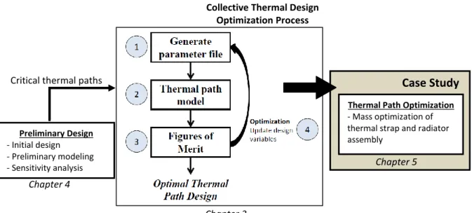
The collective thermal design optimization process shown in Figure 17 is the central methodology of this thesis. The collective thermal design optimization of the REXIS critical thermal path in Chapter 5 is completed using this optimization process. The purpose of this chapter is to explain each element in the process. Each section details one of the four steps in this process: (1) generate the parameter file of the thermal path selected for study, (2) use the thermal path model(s) to predict performance, (3) establish the FOMs and formulate the optimization problem, and (4) select an optimization algorithm and iteratively update the design variables.

The first step is to generate a parameter file for the problem. The parameter file contains specified mathematical and physical characteristics of the system that are required to generate model predictions. Parameterization of the problem occurs only once: prior to the

implementation of an optimization algorithm. Parameters include material properties and Figure 17: Collective thermal design optimization process