The Data Science Machine:
Emulating Human Intelligence in Data Science
Endeavors
by
Max Kanter
Submitted to the Department of Electrical Engineering and Computer
Science
in partial fulfillment of the requirements for the degree of
Master of Engineering in Electrical Engineering and Computer Science
at the
MASSACHUSETTS INSTITUTE OF TECHNOLOGY
June 2015
c
○ Massachusetts Institute of Technology 2015. All rights reserved.
Author . . . .
Department of Electrical Engineering and Computer Science
May 22nd, 2015
Certified by . . . .
Kalyan Veeramachaneni
Research Scientist
Thesis Supervisor
Accepted by . . . .
Prof. Albert R. Meyer
Chairman, Masters of Engineering Thesis Committee
The Data Science Machine:
Emulating Human Intelligence in Data Science Endeavors
by
Max Kanter
Submitted to the Department of Electrical Engineering and Computer Science on May 22nd, 2015, in partial fulfillment of the
requirements for the degree of
Master of Engineering in Electrical Engineering and Computer Science
Abstract
Data scientists are responsible for many tasks in the data analysis process including formulating the question, generating features, building a model, and disseminating the results. The Data Science Machine is a automated system that emulates a human data scientist’s ability to generate predictive models from raw data.
In this thesis, we propose the Deep Feature Synthesis algorithm for automatically generating features for relational datasets. We implement this algorithm and test it on 3 data science competitions that have participation from nearly 1000 data science enthusiasts. In 2 of the 3 competitions we beat a majority of competitors, and in the third, we achieve 94% of the best competitor’s score.
Finally, we take steps towards incorporating the Data Science Machine into the data science process by implementing and evaluating an interface for users to interact with the Data Science Machine.
Thesis Supervisor: Kalyan Veeramachaneni Title: Research Scientist
Acknowledgments
There a lot of people that made this thesis possible.
First, I’d like to acknowledge my adviser, Kalyan. When I started working with him well over a year ago as an undergraduate researcher, I had never worked on a research project at MIT. Reflecting now on all the time I’ve now spent in lab, it’s easy to remember so many moments where his knowledge and passion inspired and led me. I’m truly grateful for all of his key ideas that positively impacted the direction of this thesis.
I’d especially like to thank my parents for being my biggest supporters. Feeling their continued encouragement and love has meant an immeasurable amount to me over the years. Without their good example, I wouldn’t be turning in this thesis today.
Also, thank you to my labmates for being a pleasure to work with this year. I really enjoyed our conversations and the breaks we took to play pool in the CSAIL Recreation Zone. I’m excited to see what the future has in store for everyone.
Finally, I must say thank you to everyone I’ve lived with on Burton Third over the last four years. All the late nights and good memories have made my time at MIT very special.
Contents
1 Introduction 17
1.1 What is Data Science? . . . 18
1.2 Why automate? . . . 20
1.3 Contributions . . . 21
2 Overview 23 2.1 Design Goals . . . 24
3 Deep Feature Synthesis: Artificial Intelligence 27 3.1 Motivating Deep Feature Synthesis . . . 27
3.2 Deep Feature Synthesis algorithm . . . 29
3.2.1 Mathematical operators/functions . . . 29
3.2.2 Feature synthesis . . . 30
3.2.3 Recursion for relational features synthesis . . . 32
3.3 Deep Feature Synthesis: recursive algorithm . . . 33
3.4 Summary . . . 35
4 Deep Feature Synthesis: System Engineering 37 4.1 Platform . . . 37
4.2 Example . . . 39
4.3 Features: functions, storage, naming and metadata . . . 41
4.3.1 Feature Functions . . . 41
4.3.3 Naming features . . . 43 4.3.4 Metadata . . . 44 4.4 Filtering data . . . 44 4.5 Generating queries . . . 46 4.6 User configuration . . . 48 4.6.1 Dataset level . . . 48 4.6.2 Entity level . . . 48 4.6.3 Feature level . . . 49 4.7 Summary . . . 50
5 Predictive Machine Learning Pipeline 51 5.1 Defining a prediction problem . . . 51
5.2 Feature assembly framework . . . 52
5.3 Reusable machine learning pathways . . . 53
5.4 Summary . . . 56
6 Parameter Tuning 57 6.1 Bayesian parameter optimization using Gaussian Copula Processes . . 57
6.1.1 Model-Sample-Optimize . . . 58 7 Human-Data Interaction 61 7.1 Features . . . 62 7.2 Pathway parameters . . . 63 7.3 Experiments . . . 64 8 Experimental Results 65 8.1 Datasets . . . 65
8.2 Deep Feature Synthesis . . . 67
8.3 Parameter tuning . . . 67
9 Discussion 73
9.1 Creating valuable synthesized features . . . 73
9.2 Auto tuning effectiveness . . . 74
9.3 Human value . . . 76
9.4 Human-data interaction . . . 77
9.5 Implications for Data Scientists . . . 78
10 Related Work 81 10.1 Automated feature engineering . . . 81
10.2 Working with related data . . . 82
10.3 End-to-end system . . . 83
11 Conclusion 85 11.1 Future work . . . 85
List of Figures
1-1 A typical data science endeavor. Previously, it started with an ana-lyst positing a question: Could we predict if 𝑥 or 𝑦 is correlated to 𝑧? These questions are usually defined based on some need of the business or entity holding the data. Second, given a prediction problem, a data engineer posits explanatory variables and writes scripts to extract those variables. Given these variables/features and representations, the ma-chine learning researcher builds models for given predictive goals and iterates over different modeling techniques. Choices are made within the space of modeling approaches to identify the best generalizable ap-proach for the prediction problem at hand. A data scientist can span the entire process and take on the entire challenge: that is, positing the question and forming variables for building, iterating, and validating the models. . . 19
2-1 An overview of the process to automatically analyze relational data to produce predictions. The input to the system is a relational database, and the output is a predictions for a prediction problem. The predic-tion problem may be supplied by the user or determined automatically. The system achieves this using the Deep Feature Synthesis algorithm which is a capable of automatically generating features for machine learning algorithms to use. Parameters of the system are automati-cally optimized to achieve generalized performance across a variety of problems. . . 23
3-1 The data model for the KDD Cup 2014 problem. There are 9 entities. 28 3-2 An example of backward and forward relationship. In this
exam-ple, projects entity has a backward relationship with donations entity. There are multiple donations for the same project. While donations entity has a forward relationship with the projects. . . 32
4-1 The mapping of abstractions in the Data Science Machine. . . 39 4-2 An illustration of relationship between the three entities in KDD cup
2014: Projects (Pr), Donations(Do) and Donors (Dr). Projects have a backward relationship with donations (since a project may have mul-tiple donations), a donor has a backward relationship with donations (since a donor can be associated with with multiple donations). . . . 40
5-1 Reusable parameterized machine learning pipeline. The pipeline first performs truncated SVD (TSVD) and selects top 𝛾 percent of the fea-tures. Then for modeling there are currently two paths. In the first a random forest classifier is built and in the second one the training data is first clustered into k clusters and then a random forest classifiers is built for every clusters. The list of parameters for this pipeline are presented in Table 5.1. In the next section we present an automatic tuning method to tune the parameters to maximize cross validation accuracy. . . 53
6-1 Illustration of transformation of the output value 𝑓 (¯𝑝). The trans-formed value is then modeled by the regular Copula process. . . 59
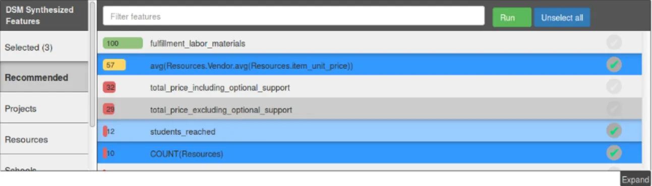
7-1 The dialog users first see when they begin using the Data Science Machine. . . 62 7-2 The feature selector component of the interface where users can choose
features to build a predictive model with. . . 63 7-3 Interface for users to modify pathway parameters . . . 63
7-4 Interface for user to view experiments. Experiments are started in the background and the score is populated when they finish. . . 64
8-1 Three different data science competitions held during the period of 2014-2015. On the left is the data model for KDD Cup 2014, at the bottom center is the data model for IJCAI, and on the right is the data model of KDD Cup 2015. A total of 906 teams took part in these competitions. We note that two out of three competitions are ongoing and predictions from the Data Science Machine solution were submitted and the results are reported in this paper. . . 66 8-2 the maximum cross validation AUC score found by iteration for all
three datasets. From top to bottom: KDD Cup 2014, IJCAI, KDD Cup 2015 . . . 68 8-3 AUC scores vs % participant achieving that score. The vertical line
indicates where the Data Science Machine ranked, From top to bottom: KDD Cup 2014, IJCAI, KDD Cup 2015 . . . 71
9-1 The cumulative number of submissions made as leader board rank in-creases in KDD Cup 2014. We can see the total number of submissions made by competitors increased exponentially as we move up the leader board. . . 76
List of Tables
3.1 Rich features extracted when recursive feature synthesis algorithm is used on the KDD Cup 2014 dataset. In this table we give the example of the computation and a simple English explanation and intuition that may actually lead the data scientist to extract the feature from the data for a particular project. . . 33
5.1 Summary of parameters in the machine learning pipeline. These pa-rameters are tuned in automatically by the Data Science Machine. . . 53
8.1 The number of rows per entity in each dataset. The uncompressed sizes of the KDD Cup 2014, IJCAI, and KDD Cup 2015 are approximately 3.1 GB, 1.9 GB, and 1.0 GB, respectively. . . 67
8.2 The number of synthesized features per entity for in each dataset. . . 68
8.3 Optimized pathway parameters from running GCP by dataset . . . . 69
8.4 The AUC scores achieved by the Data Science Machine. The "Default" score is the score achieved using the default parameters for the machine learning pathway. The "Local" score is the result of running k-folds (k=3) cross validation on the training set. The "Online" score is the score received when the result was uploaded for assessment by the competition. . . 70
8.5 How the Data Science Machine compares to human efforts. "% of Best" is the proportion of the best score the Data Science Machine achieved. "% Better" indicates the percentage of teams that out performed the Data Science Machine submission, while "# Submissions worse" is the count of all submissions made by teams that the Data Science Ma-chine outperformed. To calculate "# Days Saved", we used the rule in KDD Cup 2014 and KDD Cup 2015 that teams could make up to 5 submissions a day. Using this rule, we make a lower bound estimate of the number of days spent by teams that rank below the Data Science Machine. We do not have data on number of submissions for IJCAI. KDD Cup 2015 is still an on going competition, so this is a snapshot from May 18th, 2015. . . 70
Chapter 1
Introduction
Data science is an endeavor of deriving insights, knowledge, and predictive models from data. The endeavor also includes cleaning and curating at one end with dissemi-nation of results at the other. Data collection and assimilation methods are sometimes included. Subsequent to development and proliferation of systems and software that are able to efficiently store, retrieve, and process data, attention has now shifted to analytics, both predictive and correlative. As a result, the number of scientists that companies are looking to hire has increased exponentially [1]. To address the im-mense shortage of data scientists, businesses are resorting to any means of acquiring data science solutions. Prominent among them is crowd sourcing. Kaggle and other well-reputed data science conferences have become venues for organizing predictive analytics competitions. For example, during the course of writing this thesis, three top-tier machine learning conferences, IJCAI, ECML and ACM-RecSys1, have re-leased datasets and announced competitions for building accurate, and generalizable predictive models. This is in addition to the ACM KDD cup organized by SIGKDD every year. Hence, our goal is to make these endeavor more efficient, enjoyable, and successful.
Many of these challenges posited either on Kaggle or via conferences have a few common properties. First, the data is structured and relational, usually presented
1IJCAI is the International Joint Conference on Artificial Intelligence. ECML is the European
as a set of tables with relational links. Second, the data captures some aspect of human interactions with a complex system. Third, the presented problem attempts to predict some aspect of our behavior, decisions, or activities (e.g., to predict whether a customer will buy again after a sale [IJCAI], whether a project will get funded by donors [KDD Cup 2014], or even taxi ride destinations [ECML]). In this thesis, we argue that data science endeavors for relational, human behavioral data remain iterative, human-intuition driven, challenging, and hence, time consuming.
1.1
What is Data Science?
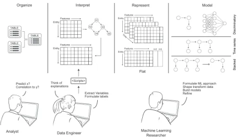
To understand the challenges of an end-to-end data science endeavor for this type of data, we next ask: What does a typical data scientist do? and What steps does it entail?. To answer these questions, we draw from numerous data science exercises of our own, and in Fig. 1.1, we present the multiple activities a data scientist does when given a linked (relational) data source for working through a typical data science endeavor. Based on this, we delineate the following steps a data scientist takes:
Formulation of a question: The first task is to formulate an impactful question, either predictive or correlative. This is often an iterative process in itself. As-sessment of whether or not the data could answer the question or whether the predictive problem defined is valuable often go hand-in-hand; therefore, it is of-ten helpful to know apriori that the information needed to solve the predictive problem is in the captured data.
Feature synthesis: The next task is forming variables, otherwise known as features. This task is iterative in nature. The data scientist may start by using some static fields (e.g., gender, age, etc.) from the tables as features, then form some specialized features based on intuition of what might predict the outcome. With these simple features at hand, the scientist may, for example, resort to features that transform these raw features into a different space-percentile of a certain feature. The result of this step is usually an entity-feature matrix, which has
Organize
Analyst
<Scripts> Think of explanations
Data Engineer Machine LearningResearcher
Formulate ML approach Shape transform data Build models Refine Extract Variables Formulate labels Predict x? Correlation to y? Interpret Model Ti m e series Discriminatory Stacked Represent Flat t=2 t=3
Figure 1-1: A typical data science endeavor. Previously, it started with an analyst positing a question: Could we predict if 𝑥 or 𝑦 is correlated to 𝑧? These questions are usually defined based on some need of the business or entity holding the data. Second, given a prediction problem, a data engineer posits explanatory variables and writes scripts to extract those variables. Given these variables/features and representations, the machine learning researcher builds models for given predictive goals and iterates over different modeling techniques. Choices are made within the space of modeling approaches to identify the best generalizable approach for the prediction problem at hand. A data scientist can span the entire process and take on the entire challenge: that is, positing the question and forming variables for building, iterating, and validating the models.
entities such as transactions, trips, customers as rows and features/variables as columns. If the data is longitudinal in nature, the matrix is assembled for each time slice.
Solve and refine using the machine learning approach: Once features are synthesized, the data scientist uses a machine learning approach. If the problem is of classification, a number of feature selection and classification approaches are available. The scientist may engage in classification methodology selection (svm, neural networks, etc.) and fine tune parameters. For a longitudinal problem, an alternative approach can be developed based on hidden Markov models and/or a stacked model where state probabilities from the learned hidden Markov model are used as features. Another alternative often pursued is to cluster the data and build cluster-wise models. In this step, one also engages in testing, validating, and reporting accuracy of the predictive model.
Communicate and disseminate results: Finally, the data scientist engages in disseminating outcomes and results. This often is beyond just predictive accu-racy and involves identifying variables that were most predictive, interpreting the models, and evaluating model accuracy under a variety of scenarios, for example, different costs for false positives and negatives.
1.2
Why automate?
Through this thesis, we ask the following foundational questions: “Can we build a machine to perform most data science activities?”, “What sort of technologies and steps are required to be able to automate these activities?”, “How could automation aid in better discovery and enable people to have better and more rewarding interactions with the data?”, “If built, how shall we measure success in developing a general-purpose data science machine?”. If such a machine is built, identifying the roles humans/scientists will play is also critical.
and modeling could be automated, albeit that automation exposes many choices. To demonstrate this, we first present an automatic feature synthesis algorithm we call Deep Feature Synthesis. We show that while being automatic in nature, the algorithm captures features that are usually supported by human intuition. Once such features are generated for a dataset, we can then formulate questions, such as: “Is this feature correlated with other features?" or “Can this subset of features predict the value for this feature?". When a time series is present in the data, we can ask, “Can we predict the future value of a particular time series?" These automated question generation mechanisms can, to a significant degree, create many questions that may be of interest to human who is trying to understand the data.
Once data is represented as variables with a supervised prediction problem, much data analysis could be automated. For example, once data is assembled and organized, we can invoke a classification system to build a classifier. If we have a time series problem, we can use a hidden Markov model, train the model, and use it to make predictions.
1.3
Contributions
The contributions in this thesis are as follows:
1. Designed Deep Feature Synthesis algorithm that is capable of generating fea-tures that express a rich feature space
2. Developed an end-to-end Data Science Machine with can
(a) posit a data science question
(b) automatically generate features via Deep Feature Synthesis
(c) autotune a machine learning pathway to extract the most out of synthe-sized features
3. Matched human level performance competing in data science competition using the Data Science Machine
4. Designed and implemented an interface to test new challenges in human-data interaction
Chapter 2
Overview
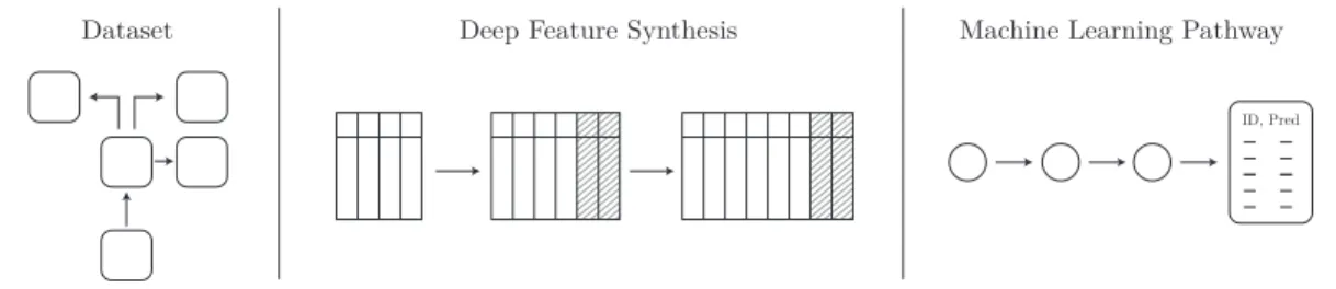
The Data Science Machine is a automated system for generating predictive models from raw data. It starts with data in the form of a relational database and automat-ically generates features to be used for predictive modeling. Most parameters of the system are optimized automatically in pursuit of good general purpose performance. Figure 2-1 shows an overview of the of the system.
Dataset Deep Feature Synthesis Machine Learning Pathway
ID, Pred
Figure 2-1: An overview of the process to automatically analyze relational data to produce predictions. The input to the system is a relational database, and the output is a predictions for a prediction problem. The prediction problem may be supplied by the user or determined automatically. The system achieves this using the Deep Feature Synthesis algorithm which is a capable of automatically generating features for machine learning algorithms to use. Parameters of the system are automatically optimized to achieve generalized performance across a variety of problems.
2.1
Design Goals
The Data Science Machine has ambitions in artificial intelligence, systems engineering, and human-data interaction. In this thesis, we aim to achieve all three of these ends. Approaching all three domains is necessary to successfully explore a new paradigm of data science. Without accomplishing our artificial intelligence goals we cannot design useful abstractions. If there is no effort put into a generalizable implementation, it would be difficult to iterate towards better designs of the AI system. Finally, if we do not consider how humans interact with the system, we would not have a way to fit the Data Science Machine in to the lives of data scientists. Because this research spans various disciplines of computer science, it challenged us to critically assess our priorities at each stage.
Artificial Intelligence Goal: Emulate human actions in data science endeavors We must design an approach that emulates the same expertise of human data scientists. The most important aspect of this is to develop a way to synthesize features that best describe the data. In Chapter 3, we describe the Deep Fea-ture Synthesis algorithm. Then, in Chapter 5 we discuss how to employ these features to solve a particular data science problem.
System Level Goals: Automate processing An implementation serves the pur-pose of testing our theories in practice. By automating the process from start to finish, we can learn more, improve our design faster, and test the system on real world problems. In Chapter 4, we discuss the implementation of the Deep Feature Synthesis. In Chapter 6, we present an automated method for parameter tuning that enables the full pathway to work.
Human-Data Interaction: Enable human creativity We must communicate how the system functions to help users learn how to interact with it. A user can know the inputs and outputs of the system, but exposing the right parts of the inner workings of the system will enable us to tap into human intelligence. We present a step towards realizing this goal in Chapter 7.
Ultimately, the greatest challenge the Data Science Machine faces is to gener-alize across a variety of problems, datasets, and situations. Without touching all components of the data science process, it would fall short of this goal.
Chapter 3
Deep Feature Synthesis: Artificial
Intelligence
The efficacy of a machine learning algorithm relies heavily on the input features [11]. Transforming raw data into useful features for a machine learning algorithm is the challenge known as feature engineering. Data scientists typically rely on their past experience or expert knowledge when brainstorming features. However, the time and effort it takes to implement a feature idea puts constraints on how many ideas are explored and which ideas are explored first. As a result, data scientists face the challenge of not only determining which ideas to implement first, but also when to stop trying ideas in order to focus on other parts of their job. Deep Feature Synthesis is the result of decomposing the features that data scientists construct into the generalized processes they follow to make them. In this Chapter, we explain the motivations for Deep Feature Synthesis, explain the feature generation abstractions, and present the pseudocode for running Deep Feature Synthesis.
3.1
Motivating
Deep Feature Synthesis
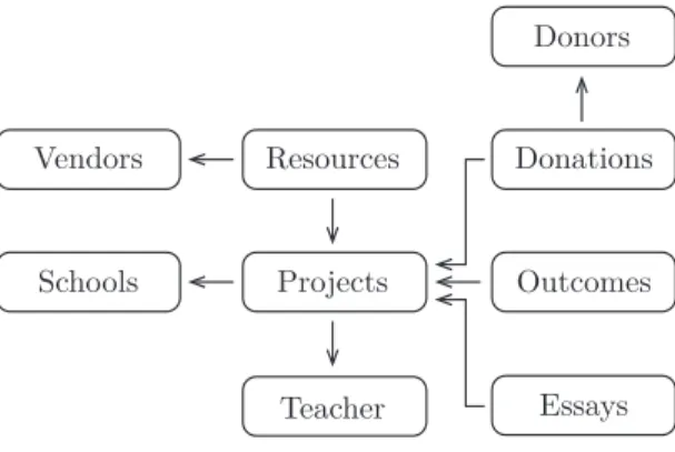
To explain various components of our system, we make use of example data problems. In this example, we look at the dataset for the KDD Cup 2014. In Figure 3-1, we see the 9 related entities in the dataset and how they are related. The entities
are projects, schools, teachers, donations, donors, resources, vendors, essays, and outcomes. Projects are associated with one school, one teacher, one essay and a set of donations. Each donation is made by a specific donor. Every project has a outcome that contains details for fundraising campaigns that have completed. The goal is to predict whether or not a particular project is exciting (as specified by the Outcome entity) before knowing any information about its funding. To do this, data scientists first resort to generating features that can be used a predictors in the model
Donors
Teacher Resources
Vendors Donations
Schools Projects Outcomes
Essays
Figure 3-1: The data model for the KDD Cup 2014 problem. There are 9 entities.
If we are to think like a data scientist, we might start by asking questions that could be translated into features that describe a project. There are several questions we could ask, but a reasonable line of questioning might be: "how much money is this project requesting?", "is that amount of money more or less than average?", "do projects started in some part of the school year perform better than others?" We might also look at entities related to a project and ask questions about them. For instance, "do successful past projects by the same school or teacher make it more likely that this project will be successful?" or "does the average income of students’ families at the school related to projects success?". These questions are then turned into features by following relationships, aggregating values, and calculating new features. Deep Feature Synthesis is a algorithm that can generate the calculations that result in these types of feature or can as proxy quantities to these ideas.
3.2
Deep Feature Synthesis algorithm
The input to Deep Feature Synthesis is a set of interconnected entities. Each entity has a primary key, which is a unique identifier for each instance of an entity that the table is based on. Optionally, an entity has a foreign key, which uniquely references an instance of a related entity. An instance of the entity has fields which fall into one the following data types: numeric, categorical , timestamps and freetext .
Notationally, for a given database, we have entities given by 𝐸1...𝐽, where each entity table has fields which we denote by 𝑥1...|𝐸𝑗|. ⃗𝑥𝑖𝑗 represents the array of values
for field 𝑖 in entity 𝑗. Each value in this array corresponds to an instance of the entity 𝑗. ⃗𝑓𝑖𝑗 represents an array that contains the feature values generated from values of field 𝑖 in entity 𝑗.
3.2.1
Mathematical operators/functions
Our feature synthesis algorithm relies on commonly used mathematical operations and functions that used by data scientists to generate features. We formalize these types of mathematical functions below. With this formalization, we allow extensibility as more functions can be added. Given a library of these functions we will next present how to apply these functions to synthesize features and provide examples for the dataset above.
Direct: These functions do a direct translation of a field to a feature. Often times this simple translation includes operations like conversion of a categorical string datatype to a unique numeric value, which could then be used as a feature. In other cases, it is simply an exact reflection of a numerical value. Hence the input to these functions is a vectors ⃗𝑥𝑖𝑗 and it returns ⃗𝑓𝑖𝑗, where ⃗𝑓𝑖𝑗 = 𝑑( ⃗𝑥𝑖𝑗), where 𝑑 is the direct computation function.
Simple: These are predefined computation functions that translate an existing field in an entity table into another type of value. Some example computations are the translation of a time stamp into 4 distinct features - weekday (1-7), day of
the month (1-30/31), month of the year (1-12) or hour of the day (1-24). Hence this transformation is given by { ⃗𝑓1
𝑖𝑗, . . . ⃗𝑓𝑖𝑗𝑘} = 𝑠( ⃗𝑥𝑖𝑗), that is when passed of array of values for field 𝑥𝑖𝑗 it returns a set of 𝑘 features for each entity. Other examples of such simple computation functions are binning a numeric value into a finite set of discrete bins.
cdf : Cumulative distribution function based features form a density function over ⃗
𝑥𝑖𝑗, and then for each entry in ⃗𝑥𝑖𝑗, they evaluate the cumulative density value ( a. k. a. percentile) thus forming a new feature 𝑓𝑐𝑑𝑓 = 𝑐𝑑𝑓 ( ⃗𝑥𝑖𝑗) (𝑖𝑗 is dropped in the notation for 𝑓 for convenience). We can also extract cumulative density in a multivariate sense given by 𝑓𝑐𝑑𝑓 = 𝑐𝑑𝑓 ( ⃗𝑥𝑖, ⃗𝑥𝑗).
r-agg: Relational aggregation features (r-agg) are derived for an instance 𝑒𝑗 of entity 𝐸𝑗 by applying a mathematical function to 𝑥𝑖𝑙|𝑒⃗ 𝑗 which is a collection of values
for field 𝑥𝑖 in related entity 𝐸𝑙, where the collection is assembled by extracting all the values for field 𝑖 in entity 𝐸𝑙 which are related to the instance 𝑒𝑗 in Entity 𝐸𝑗. This transformation is given by 𝑟 − 𝑎𝑔𝑔( ⃗𝑥𝑖𝑙|𝑒𝑗). Some examples of
r-agg functions are min, max, and count.
r-dist: r-dist features are derived from the conditional distribution 𝑃 (⃗𝑥𝑖𝑙|𝑒𝑗). These
are usually different moments of the distribution. Examples include: mean, median, std among others.
3.2.2
Feature synthesis
Next we apply these mathematical functions at two different levels: at the entity level and at the relational level. Consider an entity 𝐸𝑗 for which we are assembling the features. Below we present the two levels and examples.
Entity level: These are features calculated by solely considering the fields values in the table corresponding to the entity 𝑗 alone. In this situation, we can apply direct, simple, and cdf operations on each of the fields in the table. Figure 3-2 shows the expansion of the original entity with features { ⃗𝑓1, . . . ⃗𝑓𝑘} by applying
these operations. At this level we cannot apply r-agg and r-dist operations since we are not considering any of the relationships this entity has with other entities in the dataset.
Example 3.2.1 For the project entity, examples of these features are day-of-the-week the project was posted or percentile relative to other projects of total students reached.
Relational level: These features are derived by jointly analyzing a related entity 𝐸𝑙 to the entity 𝐸𝑗 currently under consideration. There are two possible cat-egories of relationships between these two entities: forward and backward. An illustration of these two types of relationships is shown in Figure 3-2
Forward:A forward relationship is between an instance of entity 𝐸𝑗, 𝑒𝑗, and a single instance of another entity 𝐸𝑙. This is considered the forward relationship because 𝑒𝑗 has an explicit dependence on 𝑒𝑙. In this case we can apply direct operations on the fields 𝑥1 ... 𝑥|𝐸𝑙| in 𝐸𝑙 and add them
as features of 𝐸𝑗. This is logical because an instance 𝑒𝑗 uniquely refers to a single 𝑒𝑙 meaning that all fields of 𝑒𝑙 are also legal features for 𝑒𝑗. Backward: The backward relation is the relationship from an instance 𝑒𝑗 to all
instances 𝑒𝑖 that have forward relationship to 𝑒𝑗. In the case of backward relation, we can apply r-agg and r-dist operations. These function are appropriate in this relationship because every target entity has a collection of values associated with it in the related entity.
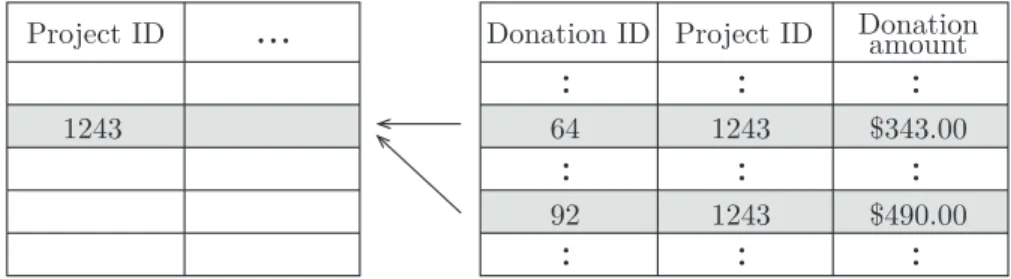
Example 3.2.2 For a project, let us consider the entity school that has a backward relationship with projects. That is, teachers and schools can be associated with multiple projects. An example of a relational level feature is then the number of projects associated with each school, evaluated us School.COUNT(Projects). Another feature could be the average number of students reached, and total number of students reached by projects for this school.
Project ID Donation ID Donationamount 1243 64 92 $343.00 $490.00
...
..
..
..
..
..
..
..
..
..
Project ID 1243 1243Figure 3-2: An example of backward and forward relationship. In this example, projects entity has a backward relationship with donations entity. There are multiple donations for the same project. While donations entity has a forward relationship with the projects.
3.2.3
Recursion for relational features synthesis
Now, what if before we created all these features for the project entity, we created features for every entity related to Projects? If features for donors and donations are made first, we would add the following feature:
Example 3.2.3 Of the donors to this project, the average number of donations by
each donor across all projects. This is evaluated as AVG(Donations.Donor.COUNT(DONATIONS)).
Table 3.1 presents some features generated by recursively extracting features for the projects. We can see that computing features as above for each of the related enti-ties first before computing the features for each project may create richer features. Generically, let us consider three related entities. That is, consider entity 𝐸𝑗 that has a relationship with entity 𝐸𝑙 that has a relationship with entity 𝐸𝑝. To define this relationship, we define a notion of depth. 𝐸𝑝 is at depth 2 with regards to entity 𝐸𝑗.
Mathematical Expression Language Expression and intuition
SUM(Donations.Donor.COUNT(DONATIONS)) The total number donations across all
projects made by donors to this project
AVG(Donations.Donor.COUNT(DONATIONS)) Of the donors to this project, the average
number of donations by each donor across all projects
SUM(Donations.Donor.SUM(Donations.amount)) The total amount donated across all
projects by donors to this project
AVG(Donations.Donor.SUM(Donations.amount)) For the donors to this project, the average
total amount donated across all projects
AVG(Donations.Donor.AVG(Donations.amount)) The average donation amount donors to
this project made on average to all projects. Intuition: Did they donate more to this project then they do on average?
Table 3.1: Rich features extracted when recursive feature synthesis algorithm is used on the KDD Cup 2014 dataset. In this table we give the example of the computa-tion and a simple English explanacomputa-tion and intuicomputa-tion that may actually lead the data scientist to extract the feature from the data for a particular project.
3.3
Deep Feature Synthesis: recursive algorithm
Next we describe the recursive algorithm to generate to generate feature vectors for a target entity. Consider that the dataset has 𝑀 entities, denoted as 𝐸1...𝑀. Let us consider that our goal is to extract features for the entity 𝐸𝑖.
To generate the features for a given entity 𝐸𝑖, we first identify all the entities with which this entity has forward relationship with and all the entities with which this entity has backward relationship with. These are denoted by sets 𝐸𝐹 and 𝐸𝐵. We must then recursively call the feature generation for all entities 𝐸𝐵 that are in backward relationship. While it is traversing through the graph of backward
relationships the algorithm keeps track of the entities it already visited in the set 𝐸𝑉.
Algorithm 1 Generating features for target entity
1: function Make_Features(𝐸𝑖, 𝐸1:𝑀, 𝐸𝑉) 2: 𝐸𝑉 = 𝐸𝑉 ∪ 𝐸𝑖 3: 𝐸𝐵 = Backward(𝐸𝑖, 𝐸1...𝑀) 4: 𝐸𝐹 =Forward(𝐸𝑖, 𝐸1...𝑀) 5: for 𝐸𝑗 ∈ 𝐸𝐵 do 6: Make_Features(𝐸𝑗, 𝐸1...𝑀, 𝐸𝑉) 7: 𝐹𝑗 =RFeat(𝐸𝑖, 𝐸𝑗) 8: 𝐹𝑖 =EFeat(𝐸𝑖) 9: for 𝐸𝑗 ∈ 𝐸𝐹 do 10: if 𝐸𝑗 ∈ 𝐸𝑉 then 11: exit 12: Make_Features(𝐸𝑗, 𝐸1...𝑀, 𝐸𝑉) 13: 𝐹𝑖 = 𝐹𝑖∪ REFLECT(𝐸𝑖, 𝐸𝑗)
The algorithm pseudocode for Make_Features is presented above. The algo-rithm stores and returns enough information to calculate the synthesized feature. This information includes not only feature values, but also metadata about base feature and function that were combined,
Next, we present Rfeat, which describes how relational features are generated given two entities 𝐸𝑖 and 𝐸𝑗 where 𝐸𝑖 has a backward relationship with 𝐸𝑗. We assume that there are set of relational level functions ℛ that can be applied. Some are describe in Section 4.3.1
Algorithm 2 Generating relational features
1: function Rfeat(𝐸𝑖, 𝐸𝑗)
2: 𝐹𝑖 = {}
3: for ∇ ∈ ℛ do
4: for 𝑥𝑗 ∈ 𝐸𝑗 do
5: if Canapply(∇, 𝑥𝑗) then 𝐹𝑖 = 𝐹𝑖∪ ∇(𝐸𝑖, 𝐸𝑗)
To apply relational level features for entity 𝐸𝑖 using entity 𝐸𝑗, Deep Feature Syn-thesis looks at all r-agg and r-dist functions that are defined in the Data Science Machine denoted by the set ℛ. It then determines which columns to apply these functions to. To do this it first iterates through functions ∈ ℛ one by one. For each
function ∇, it looks at every feature in 𝐸𝑗 to determine if the function can be applied to that feature. If the function can be applied to the feature, it is applied and the created features are added to the set of features of 𝐹𝑖. For example, a function to take the average of another columns is defined to only be applied to numeric columns. When this function is applied to a backward relationship between 𝐸𝑖 and 𝐸𝑗, it will add the average of each numerical feature in 𝐸𝑗 to the feature set of 𝐸𝑖.
If a particular entity has a second feature it can be filtered by, Deep Feature Synthesis will apply the function multiple times, each time filtering for one of the distinct values in the second feature.
3.4
Summary
(a) It is possible to automatically generate features that have human level interpre-tation or map to human intuition.
(b) We are able to generate rich features with the recursive algorithm, Deep Feature Synthesis.
(c) By designing the proper abstractions, the algorithm is extensible with new mathematical functions.
Chapter 4
Deep Feature Synthesis: System
Engineering
Our goal when implementing Deep Feature Synthesis is to enable us to rapidly deploy the Data Science Machine and evaluate the features when it encounters a new dataset. As such, it is important to design a system that is agnostic to the dataset. Once we establish that the input to the system will be a relational database, we must address a variety of challenges to make it generalizable. In this chapter, we present th challenges that this brings about and how we address them.
As we argued in Chapter 2, having a system that can automatically generate features given a new relational dataset not only makes the system ready to be used by data scientists, but it also enables us iterate on our AI system because with each new dataset the system can be improved.
4.1
Platform
The Data Science Machine and accompanying Deep Feature Synthesis algorithm are built on top of the MySQL database using the InnoDB engine for tables. MySQL was chosen for its maturity as a database. With this choice, all raw datasets were manually converted to a MySQL schema for processing by the Data Science Machine. We implement the logic for calculating, managing, and manipulating the synthesized
features in Python.
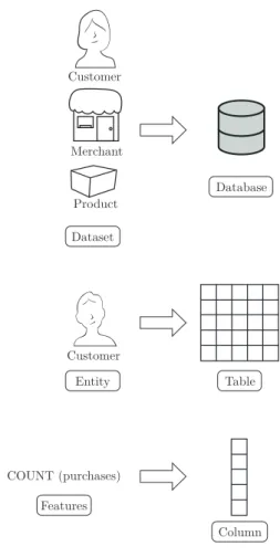
Dataset, Entity, Feature Abstractions: We chose to use a relational database due to the natural parallels in how they store data and the requirements of Deep Feature Synthesis. There are a three key components in the Deep Feature Synthesis that must be represented in the implementation. Figure 4.1 shows how those are mapped to a relational database. A dataset is represented by an entire database. Within a dataset there are several entities that represent different "objects" in the dataset. Each entity is represented by a specific table in the database. Finally, each entity contains features. A single feature is represented by a single column in the database.
When we discussed the AI component of the system we spoke in terms of datasets, entities, and features. However, when we discuss the system component, it is often convenient to speak in terms of databases, tables, and columns.
The challenges for the platform are:
What platform do we build this on? The Deep Feature Synthesis has require-ments for the type of data it must store and how it will access it. We must pick a platform that fits these requirements.
How do we represent, store, and features? The features in a dataset may vary in datatype and quantity. We need to have a general way of storing features.
How do we filter the data? There needs to be an easy way to access the data we want. Different datasets may require slicing data in different ways and our system should flexibly handle that.
How do we generate queries? We cannot have expectations for how data is la-beled and organized other than that it is in a relational database. We must be able to generate queries without making assumption about naming or organi-zation conventions.
How do we let the user help the system? Automating parts of the system may be time consuming for little practical gain. For these aspects, we should let the
Customer Customer COUNT (purchases) Merchant Product Dataset Database Entity Table Features Column
Figure 4-1: The mapping of abstractions in the Data Science Machine.
user provide information to aid the system.
4.2
Example
Let us consider an example feature for the Projects entity in the KDD Cup 2014 dataset: AVG(Donations.Donor.SUM(Donations.amount)). Ultimately, we must construct a database query that extracts this value. In this example, the final fea-ture is actually constructed using synthesized feafea-tures. To take advantage of this, our approach is to calculate and store those intermediate features rather than creat-ing a monolithic query. This allows reuse of intermediate values and simplifies the implementation.
Pr
Do
Dr
Figure 4-2: An illustration of relationship between the three entities in KDD cup 2014: Projects (Pr), Donations(Do) and Donors (Dr). Projects have a backward relationship with donations (since a project may have multiple donations), a donor has a backward relationship with donations (since a donor can be associated with with multiple donations).
Figure 4.2 shows the relationship between the three entities under consideration. The process starts with following entity relationships as described in Section 3.3. Starting with projects it recurses to the donations entity and since donations by itself does not have any backward relationships, it considers its forward relationship with donors.
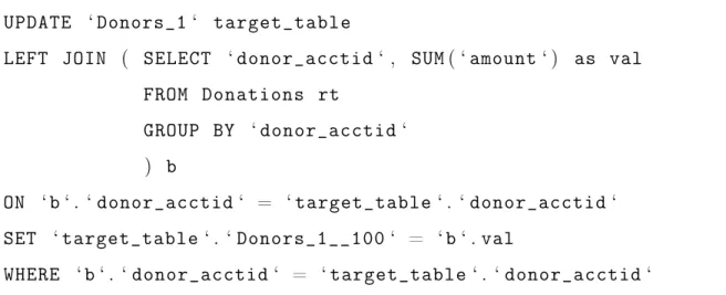
Once we reach the Donor entity, we consider its backward relationship with dona-tions and begin to apply the Rfeat algorithm presented in Section 3.3. The algorithm iterates over Feature Functions which each specify a calculation and rules about when it should be applied. At this level, when the algorithm considers SUM, the SQL query to generate features for the donors is created automatically as shown below:
UPDATE ‘ Donors_1 ‘ target_table
LEFT JOIN ( SELECT ‘ donor_acctid ‘ , SUM ( ‘ amount ‘ ) as val FROM Donations rt
GROUP BY ‘ donor_acctid ‘ ) b
ON ‘ b ‘ . ‘ donor_acctid ‘ = ‘ target_table ‘ . ‘ donor_acctid ‘ SET ‘ target_table ‘ . ‘ Donors_1__100 ‘ = ‘ b ‘ . val
WHERE ‘ b ‘ . ‘ donor_acctid ‘ = ‘ target_table ‘ . ‘ donor_acctid ‘
After calculating the feature, we store the feature values as a new column in the Donors table, as well as store the metadata to use later in the process. The metadata contains information such as the base column (Donations.amount) and the function applied (SUM). At this stage we have synthesized the feature SUM(Donations.amount),
considering all the donations that this donor has in the donations table.
With a new feature synthesized for each donor in the dataset1, we build features for each donation. Because each donation uniquely references a single donor, we just re-flect the feature we just calculated to the Donation table. When we rere-flect this feature we do not actually copy the value. Instead, using the same metadata object men-tioned above, we notate where the true feature values are actually stored. In this case, it is in the Donors table. We now have the feature Donor.SUM(Donations.amount) for every donation.
The final step is to generate features for the original entity, Projects. Now, con-sidering its backward relationship with donations, we begin to apply the AVG Feature Function (via the RFEAT algorithm). This is similar to applying the Feature Func-tion before except that the feature we want to aggregate isn’t actually stored in the entity it is associated with. However, using the information in the metadata object we know where in the database a feature is actually stored. With this information we can create a subquery that joins the appropriate tables together to make the feature columns available. After the join, we can construct the query as we did before,
If at any point, we only want a subset of of data, we use Filter Objects. For example, if we wish to calculate the same feature above, but only for Donors that live in Massachuseets, we could create a Filter Object with the triple ("state", "=", "MA"). This Filter Object is then serialized and used in the query.
4.3
Features: functions, storage, naming and
meta-data
4.3.1
Feature Functions
The functions described in 3.2.1 are implemented as Python classes, and they all provide a Feature Function interface. A Feature Function takes one or two entities as inputs depending on the type of feature. Two entities are required in the case of
1
relational level features, and direct features where the source is another entity. The function definition is responsible for determining whether or not it can be applied to a certain columns using the column’s metadata (described below 4.3.4) and how to calculate the output value. For example, some Feature Functions specify they should only be applied to date fields. Because features are often calculated using synthesised features, Feature Functions may also specify rules that govern what mathematical functions can be applied to synthesized features. For example, a rule limits the standard deviation Feature Function from being appled to a feature synthesized using the standard deviation Feature Function.
For performance reasons, the Data Science Machine builds Feature Functions on top of the functions provided by MySQL. Currently, the Data Science Machine im-plements the following relational level functions: AVG(), MAX(), MIN(), SUM(), STD(), and COUNT(). In addition to those functions, the system implements the following simple functions: length() function to calculate the number of character in a text field, WEEKDAY() to convert dates to the day of the week they occurred, and MONTH() to do the same for the month. Despite their simplicity, this small base of functions is enough to create a wide range of features for us to evaluate the Data Science Machine.
4.3.2
Feature storage
All features are stored as columns in the database. As the Data Science Machine creates new features, it uses new columns to store the data. Successively altering table columns on a large MySQL table using the ALTER TABLE command is expensive because MySQL must create a temporary copy of the original table while also locking the original [2]. Because of this overhead in creating the temporary table each time a new column is created, it is infact cheaper to create multiple columns simultaneously. Thus, while creating the first new column for a table, the Data Science Machine actually creates multiple new columns. To manage these new columns, the Data Science Machine implements a Column Broker. By default the Column Broker creates 500 new columns at a time and specifies the data types for 80% of them as floats and the rest 20% as integers. These settings are configurable using the configuration file
mentioned later in Section 4.6.
The Column Broker maintains a list of the free columns of each type. Using the Column Broker, Deep Feature Synthesis then can request a column of a fea-ture’s datatype on demand without the latency of issuing the ALTER TABLE command. Without this optimization, creating hundreds of new features would take a prohibitive amount of time.
If the Column Broker does not have a column of the requested datatype, then it will create a copy of the original table that has the same fields as the original table and initialize multiple new columns again. Even though these columns are in a separate table, by copying the original columns, we maintain the primary key information for each row. Using the primary key we can join the original table with its copies when we need access to specific features. MySQL limits InnoDB tables to have 1000 column max. Thus, without this implementation the Data Science Machine would be limited in the number of features it could synthesize for a given entity.
4.3.3
Naming features
A challenge faced by the Data Science Machine is displaying synthesized features in a human understandable way. In part, this is because simply describing a calculation does not necessarily resemble the intuitive description a human would give. The solu-tion is to use a standardized mathematical notasolu-tion. Table 3.1 shows some examples of features names and their natural language descriptions. The relationship between the name of the feature and English description is often not immediately clear.
A feature name is constructed by surrounding another feature name with the function that was applied to it. If the function is omitted, it is assumed to have been a direct function that reflected the value of the feature in a forward relationship. For example, Table 3.1 shows examples of this where Donor reflects a feature from Donations. Because the notation definition for a feature name is defined by another feature name, we get the recursive effect of functions inside functions.
4.3.4
Metadata
An important aspect to being able to use the features created by Deep Feature Syn-thesis is to understand how it came about. To accomplish this, every feature contains a metadata object.
The metadata object has the following fields:
Field Purpose
entity the entity this feature is for
real_name a name that encodes what the feature is. eg School.MAX(Projects.SUM(Dontations.total)) which means largest amount raised by a project at this school) path list of path nodes that describe how this feature was
calcu-lated
A path is a list of nodes which are defined as follows:
Field Purpose
Base column the column this feature was derived from and its metadata feature_type the type of feature this is, eg direct, r-agg, etc
feature_type_func the name of the function that was applied
filter the Filter Object used by the query that generates it.
4.4
Filtering data
The Data Science Machine needs a flexible way to select subsets of data. Filter Objects play an important role for relational level Feature Functions by enabling calculations over subsets of instances. They are implemented to enable construction of new Filter Objects by combining Filter Objects using logical operators such as “and” or “or”. Using Filter Objects, a Feature Function is able to select which instances of an entity to include in a calculation.
Filter Objects implement two methods for the query generation process described in 4.5.
1. to_where_statement(). This converts a Filter Object to a MySQl where state-ment to be included in a query. For example, FilterObject([("state", "=", "MA"), ("age", ">=", 18)]) serializes to WHERE ‘state‘ = MA AND ‘age‘ > 18.
2. get_involved_columns(). This returns all the columns that this filter will be applied to. This is used by the query generation algorithm to ensure they are selected before applying the WHERE statement.
Filter Objects are used to implement two useful pieces of functionality for Deep Feature Synthesis: conditional distributions and time intervals.
Conditional distributions Filter Objects can be used to condition a Feature Func-tion. This is important because there are many scenarios where the conditional distribution exposes important information in a dataset. A guiding example is making features for customers of an ecommerce website. Without Filter Ob-jects, Deep Feature Synthesis could create a feature for each customer that is the total amount of money that customer spent on the site by summing up all the purchases the customer made. However, this might not differentiate cus-tomers that spent the same amount of money, but in different ways. Instead, we might want to create features for the total amount spent in each of the product categories such as electronics or apparel. This is accomplished by using different Filter Objects that each select only the purchases from a single category before applying the Feature Function.
Time intervals For some prediction problems, we want to calculate the same set of features across many time intervals. This allows use to model time series data. A time interval Filter Object is implemented as a logical combination of two Filter Objects. One Filter Object selects instances that occur after a certain time and one Filter Object selects instances that occur before a certain time.
When these two functions are combined using the AND operator, they specify a single time interval.
When creating intervals there are 4 important parameters.
1. The column that stores the time interval
2. The time to start creating time intervals
3. The length of the time interval
4. The number of intervals.
When supplied with these four parameters, Deep Feature Synthesis is capable of creating time interval-based features for a target entity. Deep Feature Synthesis maintains metadata about the creation of each feature that can be used by a learning algorithm to determine the features associated with each time interval.
4.5
Generating queries
In order to extract features, the Data Science Machine constructs MySQL database queries on the fly. As the data required to calculate a feature may be stored in multiple tables, a process for joining tables together is necessary. All columns in the SELECT clause or WHERE clause of a query must be accessible for a query to work.
MySQL supports Views, which are virtual tables composed of columns from other tables or views. While these would simplify the design of the query generation, in the Data Science Machine design we choose to manually implement the logic to join tables together. We did this for two reasons. First, the workload of the Deep Feature Synthesis iteratively adds columns to tables. The changing structure of tables would mean redefining a new view each time a new column is added as MySQL views are frozen at the time of creation[3]. Second, while we may join the same tables together to make different features, we often will be selecting different columns from the joined result. To use a view for this would lead to unnecessary columns at times in our select, resulting in a potential performance hit.
To improve performance further, a query is constructed to perform multiple cal-culations at once. This works by cutting down on the number of times the query builder performs joins, as well reducing the number of times Deep Feature Synthesis has to iterate over every row in a table. A query is constructed in the following three steps:
Collect Columns The first step is determining all columns that are involved in the query. Columns may be involved in a query because they are part of the actual calculation or because the query contains a Filter Object.
Determine join path The actual source of a column may be in different table than the target of the calculation, but the column metadata stores the path to the column. Using this path data we can construct a join path, which is a series of MySQL JOIN statements that assemble a subquery for the query to execute on. If we collected multiple columns for the query, we can have many different paths, some of which share parts. The join path is constructed by first sorting the involved columns by path length. Then, starting with the longest path, we join tables in the path beginning with the table we wish to add the feature to. We proceed column by column in this sorted order. For each new column we only add tables from its path if they branch from the path that has already been constructed. By iterating over the columns according to path length, we ensure the paths with the most constraints are handled first.
Build Query With the subquery to build the joined table, the final step is to put the desired functions of the columns in a SELECT statement, turn the Filter Object into a WHERE clause using the defined API, and group by the primary key of the target entity. The GROUP BY is what collects the rows for relational level functions.
4.6
User configuration
The Data Science Machine takes a configuration file for specifying dataset specific options. The configuration file presents options at the tree levels of abstractions in the data science machine: dataset, entity, and feature. The Data Science Machine will infer some of these parameters to the best of its ability or revert to a sensible default value if inference is difficult or computational expensive.
4.6.1
Dataset level
Option Purpose
max_depth the maximum recursion depth of the deep feature synthesis algorithm
max_categorical_filter the maximum number of categorical filters to apply along a feature pathway
4.6.2
Entity level
Every entity in the dataset has a copy of the following parameters
Option Purpose
one_to_one list of entity names that are in a one-to-one rela-tionship with this entity. Since the one-to-one re-lationship goes both ways, a given pair only needs to be notated in at least one entity
included_functions white list of Feature Functions to apply to an entity excluded_functions black list of Feature Functions to apply to an entity train_filter parameters for a Filter Object that specifies which
instances of this entity may be used for training
One-to-one relationship are inferred by counting the number of backward relation-ship for every entity in a table. Backward relationrelation-ships are defined in section 3.2.2.
If the number of backward relationships is one for every instance then it is considered to be part of a one-to-one relationship. This calculation is expensive in the current system, so it is cached and only performed once for each relationship. Additionally, it is also not performed on entities that contain more the 𝑡 rows, where 𝑡 is currently set to 10 million.
If not specified, included_functions is assumed to be every function available. Therefore included_functions and excluded_functions can be used as a white list and black list for Feature Functions. Typically this is used to avoid performing expensive computations that the user expects to not contribute to successful feature generation.
4.6.3
Feature level
Every feature in the dataset has a copy of the following parameters
Option Purpose
categorical boolean indicating whether or not this variable is categorical
categorical_filter boolean indicating whether or not to use distinct values of this feature as Filter Object
numeric boolean indicating whether or not this variable is numeric
ignore boolean indicating whether or not to ignore a fea-ture. this is used when the metadata is necessary for some other computation and the column isn’t actually a feature such as label test or train data.
Categorical can often be inferred. Right now, the Data Science Machine assumes columns that have exactly two distinct values to be categorical. The Data Science Machine avoids being too liberal in calling features categorical because they lead to an growth in the feature space during the machine learning pipeline. For example, the zip code of a customer is categorical, but could create thousands of new features
during One Hot Encoding (explained in Section 5.3).
Numeric is assumed if the database column type is specified as a numeric type. This includes integers, floats, doubles, decimals, smallints, and mediumint in MySQL.
4.7
Summary
(a) We implemented Deep Feature Synthesis using MySQL and Python.
(b) The implementation make no assumptions about the input beyond it is a rela-tional database.
(c) We allow for humans to guide the system as needed with a configuration file on a per dataset basis.
Chapter 5
Predictive Machine Learning Pipeline
To use the features created by Deep Feature Synthesis, we must implement a gen-eralized machine learning path. For this, we have at our disposal a representation of the data as tuples given by < 𝑒, 𝑓 𝑛, 𝑓 𝑣, 𝑡 > where 𝑒 is entity, 𝑓 𝑛 is the feature name, 𝑓 𝑣 is the feature value, and 𝑡 is the time interval id. To build a predictive modeling framework we next design three components: an automatic prediction problem for-mulator, a feature assembly framework, and a machine learning framework. We use the open source scikit-learn [15] to aid the development of this pathway. In the next two subsections we describe these three components.
5.1
Defining a prediction problem
The first step is to formulate a prediction problem. This means selecting one of the features in the dataset to model. The feature could be one that already exists in the dataset or one that was generated while running Deep Feature Synthesis. Additionally, the feature may be a continuous value such as the the total amount of money donated by a donors or a categorical value such as whether or not a project was fully funded. We call this feature we wish to predict the target value.
For some cases, the target value is known before the analysis begin, in which case this information can be supplied to the Data Science Machine. This is the case for
the competitions we test the system on.
In other cases, when the target value is not externally provided, Data Science Machine can run the machine learning pipeline for several potential target value and suggest high performing results. To prioritize which ones to pick as target value and show the results to the user, Data Science Machine applies some basic heuristics. At this time, these heuristics are
∙ Preference for variables that are not derived via feature synthesis algorithm
∙ Categorical variables with a small number of distinct categories
∙ Numeric features with high variance
5.2
Feature assembly framework
After a target value is selected, we next assemble the features that are appropriate for use in prediction. We call these features predictors. For a given target value, some predictors might be invalid because they were calculated with the common base data or have an invalid time relationship. For instance, if the target value to predict is the average donation amount made by a donor, it would be invalid to predict that using the total amount the donor donated and the number of donations they made. A feature could invalid temporally, if it relies on the data that did not exist at the time of the target value. For example, if we want to predict how many donations a project will receive in it’s first week, it is invalid to predict that using a feature that is the total sum of the donations for that project.
To accomplish the task of assembling features for a valid prediction problem, the Data Science Machine maintains a database of metadata associated with each entity-feature. This metadata contains information about the source fields in the original database that were used to form this feature, as well as any time dependencies contained with in it. Using this metadata, the Data Science Machine assembles a list of all features that were used to calculate the target feature. The Data Science Machine makes this same list for all candidate predicting features. A feature is only usable
if these lists contain no overlaps. To handle time dependencies, the Data Science Machine excludes any feature that is assigned an interval number higher than the target feature.
5.3
Reusable machine learning pathways
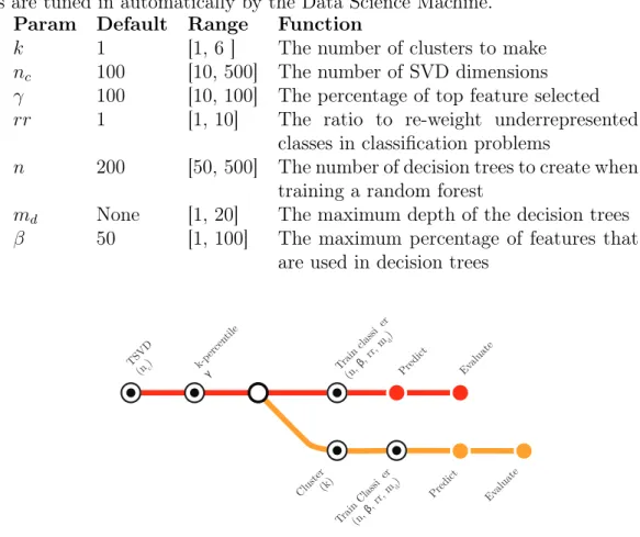
Table 5.1: Summary of parameters in the machine learning pipeline. These parame-ters are tuned in automatically by the Data Science Machine.
Param Default Range Function
𝑘 1 [1, 6 ] The number of clusters to make 𝑛𝑐 100 [10, 500] The number of SVD dimensions 𝛾 100 [10, 100] The percentage of top feature selected 𝑟𝑟 1 [1, 10] The ratio to re-weight underrepresented
classes in classification problems
𝑛 200 [50, 500] The number of decision trees to create when training a random forest
𝑚𝑑 None [1, 20] The maximum depth of the decision trees 𝛽 50 [1, 100] The maximum percentage of features that
are used in decision trees
Cluster(k) Train Classifier(n, β, rr, m d ) TSVD (n)c k-p ercen tile γ Train classifier(n, β, rr, m d ) Predict Evaluate Predict Evaluate
Figure 5-1: Reusable parameterized machine learning pipeline. The pipeline first performs truncated SVD (TSVD) and selects top 𝛾 percent of the features. Then for modeling there are currently two paths. In the first a random forest classifier is built and in the second one the training data is first clustered into k clusters and then a random forest classifiers is built for every clusters. The list of parameters for this pipeline are presented in Table 5.1. In the next section we present an automatic tuning method to tune the parameters to maximize cross validation accuracy.
With a target feature and predictors selected, the Data Science Machine imple-ments a parametrized pathway for data preprocessing, feature selection,
dimension-ality reduction, modeling, and evaluation. To tune the paramters, he Data Science Machine provides a tool for performing intelligent parameter optimization. The fol-lowing steps are followed for machine learning and building predictive models: Data preprocessing
The importance of the data preprocessing step is to normalize data before continuing along the pathway. To preprocess the data, we assemble a matrix using the tuples < 𝑒, 𝑓 𝑛, 𝑓 𝑣, 𝑡 > for the target 𝑓 𝑛 and each 𝑓 𝑛 that was chosen to be a predictor. In this matrix, each row corresponds to an instance of 𝐸 and each column contains the values 𝑓 𝑣 for the corresponding 𝑓 𝑛.
There are several steps normalize the data
∙ Null values: We must convert null values. If a feature is a continuous value, the null value is converted to the median value of the feature. If the feature is categorical, the null value is converted to an unknown class.
∙ Categorical variables: Categorical variables are sometimes represented in this matrix as string. So, first we must convert each distinct string to a distinct integer. Next, we use One Hot Encoding to convert the categorical variable into several binary variables. If there are 𝑛 classes for the categorical variable, we create n binary features in which only one is positive for each instance.
∙ Feature scaling: Different features are often at different scales depending on their unit. To prevent certain features from dominating a model, each feature column is scaled to have a mean of 0 and unit variance.
Feature selection and dimensionality reduction
Deep Feature Synthesis generates a large number of features per entity. Even after removing the features that may be invalid for predicting the target value, we are still left with a large number of predictors that we can use for predicting the target value. Many of these features may not have any predictive value, or even if they have little predictive value, could diminish the value of the good predictors because they increase the dimensionality. To overcome this, it is important to have a process of selecting the