HAL Id: hal-02975965
https://hal.archives-ouvertes.fr/hal-02975965
Submitted on 26 Oct 2020
HAL is a multi-disciplinary open access
archive for the deposit and dissemination of
sci-entific research documents, whether they are
pub-lished or not. The documents may come from
teaching and research institutions in France or
abroad, or from public or private research centers.
L’archive ouverte pluridisciplinaire HAL, est
destinée au dépôt et à la diffusion de documents
scientifiques de niveau recherche, publiés ou non,
émanant des établissements d’enseignement et de
recherche français ou étrangers, des laboratoires
publics ou privés.
choice
Andreas Plach, Kerim Nisancioglu, Sébastien Le Clec’H, Andreas Born, Petra
Langebroek, Chuncheng Guo, Michael Imhof, Thomas Stocker
To cite this version:
Andreas Plach, Kerim Nisancioglu, Sébastien Le Clec’H, Andreas Born, Petra Langebroek, et al..
Eemian Greenland SMB strongly sensitive to model choice. Climate of the Past, European Geosciences
Union (EGU), 2018, 14 (10), pp.1463-1485. �10.5194/cp-14-1463-2018�. �hal-02975965�
https://doi.org/10.5194/cp-14-1463-2018 © Author(s) 2018. This work is distributed under the Creative Commons Attribution 4.0 License.
Eemian Greenland SMB strongly sensitive to model choice
Andreas Plach1, Kerim H. Nisancioglu1,2, Sébastien Le clec’h3,4, Andreas Born1,5,6, Petra M. Langebroek7, Chuncheng Guo7, Michael Imhof8,5, and Thomas F. Stocker5,6
1Department of Earth Science, University of Bergen and Bjerknes Centre for Climate Research, Bergen, Norway 2Centre for Earth Evolution and Dynamics, University of Oslo, Oslo, Norway
3Laboratoire des Sciences du Climat et de l’Environnement, LSCE/IPSL, CEA-CNRS-UVSQ, Université Paris-Saclay, 91191 Gif-sur-Yvette, France
4Earth System Science and Department Geografie, Vrije Universiteit Brussel, Brussels, Belgium 5Climate and Environmental Physics, Physics Institute, University of Bern, Bern, Switzerland 6Oeschger Centre for Climate Change Research, University of Bern, Bern, Switzerland 7Uni Research Climate and Bjerknes Centre for Climate Research, Bergen, Norway 8Laboratory of Hydraulics, Hydrology and Glaciology, ETH Zürich, Zürich, Switzerland
Correspondence:Andreas Plach ([email protected]) Received: 3 July 2018 – Discussion started: 9 July 2018
Revised: 20 September 2018 – Accepted: 5 October 2018 – Published: 19 October 2018
Abstract.Understanding the behavior of the Greenland ice sheet in a warmer climate, and particularly its surface mass balance (SMB), is important for assessing Greenland’s po-tential contribution to future sea level rise. The Eemian in-terglacial period, the most recent warmer-than-present pe-riod in Earth’s history approximately 125 000 years ago, pro-vides an analogue for a warm summer climate over Green-land. The Eemian is characterized by a positive Northern Hemisphere summer insolation anomaly, which complicates Eemian SMB calculations based on positive degree day esti-mates. In this study, we use Eemian global and regional cli-mate simulations in combination with three types of SMB models – a simple positive degree day, an intermediate com-plexity, and a full surface energy balance model – to evaluate the importance of regional climate and model complexity for estimates of Greenland’s SMB. We find that all SMB mod-els perform well under the relatively cool pre-industrial and late Eemian. For the relatively warm early Eemian, the dif-ferences between SMB models are large, which is associated with whether insolation is included in the respective mod-els. For all simulated time slices, there is a systematic dif-ference between globally and regionally forced SMB mod-els, due to the different representation of the regional climate over Greenland. We conclude that both the resolution of the simulated climate as well as the method used to estimate the SMB are important for an accurate simulation of Greenland’s
SMB. Whether model resolution or the SMB method is most important depends on the climate state and in particular the prevailing insolation pattern. We suggest that future Eemian climate model intercomparison studies should include SMB estimates and a scheme to capture SMB uncertainties.
1 Introduction
The projections of future sea level rise remain uncertain, es-pecially the magnitude and the rate of the contributions from the Greenland ice sheet (GrIS) and the Antarctic ice sheet (Church et al., 2013; Mengel et al., 2016). In addition to im-proving dynamical climate models, it is important to test their ability to simulate documented warm climates. Past inter-glacial periods are relevant examples as these were periods of the recent past with relatively stable warm climates per-sisting over several millennia. They provide benchmarks for testing key dynamical processes and feedbacks under a dif-ferent background climate state. Quaternary interglacial pe-riods exhibit a geological configuration similar to today (e.g., gateways and topography) and have been frequently used as analogues for future climates (e.g., Yin and Berger, 2015). In particular, the most recent interglacial period, the Eemian (approximately 130 to 116 ka) has been used to better under-stand ice sheet behavior during a warm climate.
Compared to the pre-industrial period, the Eemian is es-timated to have had less Arctic summer sea ice, warmer Arctic summer temperatures, and up to 2◦C warmer annual global average temperatures (CAPE Last Interglacial Project Members, 2006; Otto-Bliesner et al., 2013; Capron et al., 2014). Ice core records from NEEM (the North Greenland Eemian Ice Drilling project in northwest Greenland) indi-cate a local warming of 8.5 ± 2.5◦C (Landais et al., 2016) compared to pre-industrial levels. However, total gas con-tent measurements from the deep Greenland ice cores GISP2, GRIP, NGRIP, and NEEM indicate that the Eemian surface elevation at these locations was no more than a few hun-dred meters lower than present (Raynaud et al., 1997; NEEM community members, 2013). Proxy data derived from coral reefs show a global mean sea level at least 4 m above the present level (Overpeck et al., 2006; Kopp et al., 2013; Dut-ton et al., 2015).
Several studies have investigated the Eemian GrIS. Nev-ertheless, there is no consensus on the extent to which the GrIS retreated during the Eemian. Scientists have applied ice core reconstructions (e.g., Letréguilly et al., 1991; Greve, 2005) and global climate models (GCMs) of various com-plexities (e.g., Otto-Bliesner et al., 2006; Stone et al., 2013) combined with regional models (e.g., Robinson et al., 2011; Helsen et al., 2013) to create Eemian temperature and precip-itation forcing over Greenland. Based on these reconstructed or simulated climates, different models have been used to cal-culate the surface mass balance (SMB) in Greenland for the Eemian. The vast majority of these studies use the positive degree day (PDD) method introduced by Reeh (1989), which is based on an empirical relation between melt and temper-ature. PDD has been shown to work well under present-day conditions (e.g., Braithwaite, 1995) and has been widely used by the community due to its simplicity and ease of integra-tion with climate and ice sheet models. More recent studies employ physically based approaches to calculate the SMB, ranging from empirical models (e.g., Robinson et al., 2010) to surface energy balance (SEB) models (e.g., Helsen et al., 2013).
It is important to note that the relatively warm summer (and cold winter) in the Northern Hemisphere during the early Eemian (130–125 ka) was caused by a different insola-tion regime compared to today, not increased concentrainsola-tions of greenhouse gases (GHGs) which are primarily respon-sible for the recent observed global warming (e.g., Lange-broek and Nisancioglu, 2014). The early Eemian was charac-terized by a positive solar insolation anomaly during north-ern summer caused by a higher obliquity and eccentricity compared to present, as well as a favorable precession, giv-ing warm Northern Hemisphere summers at high latitudes (Yin and Berger, 2010). The higher summer insolation over Greenland, compared to today, adds snow/ice melt which is not included in the PDD approach (e.g., Van de Berg et al., 2011). These limitations should be kept in mind when us-ing past warm periods as analogues for future warmus-ing (e.g.,
Ganopolski and Robinson, 2011; Lunt et al., 2013). However, the higher availability of proxy data compared to preced-ing interglacial periods makes the Eemian a better candidate to investigate warmer conditions over Greenland (Yin and Berger, 2015). Furthermore, Masson-Delmotte et al. (2011) found a similar Arctic summer warming over Greenland with the higher Eemian insolation as for a future doubling of at-mospheric CO2given fixed pre-industrial insolation.
In this study, we assess the importance of the represen-tation of small-scale climate features and the impact of the SMB model complexity (i.e., using three SMB models) when calculating the SMB for warm climates such as the Eemian. High-resolution pre-industrial and Eemian Greenland cli-mate is provided by downscaling global time slice simula-tions with the Norwegian Earth System Model (NorESM) using the regional climate model (RCM) MAR (Modèle At-mosphérique Régional). Based on these global and regional climate simulations, three different SMB models are applied, including (1) a simple, empirical PDD model, (2) an interme-diate complexity SMB model explicitly accounting for solar insolation, as well as (3) the full SEB model implemented in MAR.
A review of previous Eemian GrIS studies is given in Sect. 2, followed by the models, data, and experiment de-sign in this study discussed in Sect. 3. The results of the pre-industrial and Eemian simulations are presented in Sects. 4 and 5, respectively. The challenges and uncertainties are dis-cussed in Sect. 6. Finally, a summary of the study is given in Sect. 7.
2 Comparison of previous Eemian Greenland studies
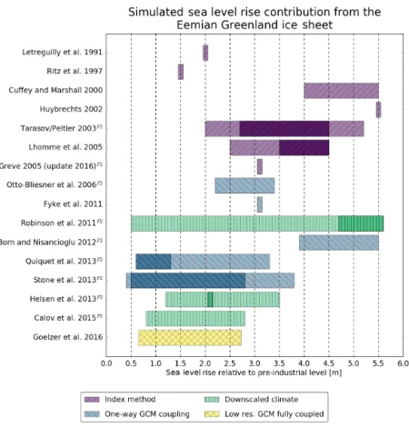
Scientists started modeling the Eemian GrIS more than 25 years ago (Letréguilly et al., 1991). However, a clear pic-ture of the minimum extent and the shape of the Eemian GrIS is still missing. The estimated contributions from the GrIS to the Eemian sea level rise differ largely and vary be-tween 0.4 and 5.6 m. An overview of previous studies and their estimated Eemian sea level rise from Greenland is given in Fig. 1.
Early studies used Eemian temperature anomalies derived from ice core records and perturbed a present-day temper-ature field in order to get estimated Eemian tempertemper-atures over Greenland. This index method was either based on single Greenland ice cores (Letréguilly et al., 1991; Ritz et al., 1997) or a composite of ice cores from Greenland and Antarctica (Cuffey and Marshall, 2000; Huybrechts, 2002; Tarasov and Peltier, 2003; Lhomme et al., 2005; Greve, 2005). All these “index studies” employed a present-day pre-cipitation field for modeling Eemian Greenland. This empir-ical approach was followed by the usage of climate models. The first studies used GCM output directly to force SMB models (Otto-Bliesner et al., 2006; Fyke et al., 2011; Born
and Nisancioglu, 2012; Stone et al., 2013). Later studies used statistical (Robinson et al., 2011; Calov et al., 2015) and dynamical downscaling of GCM simulations (Helsen et al., 2013) to create climate input for SMB models. Quiquet et al. (2013) used an adapted index method employing Eemian temperature and precipitation anomalies from two GCMs.
Various ice sheet models were used in these studies to es-timate the Eemian ice sheet evolution. However, all ice sheet models used are based on similar ice flow equations – either the shallow ice approximation (SIA) or a combination of the SIA and the shallow shelf approximation (SSA). Therefore, the choice of the ice sheet model cannot explain the differ-ences between these studies, and hence the ice dynamics is not discussed further. For more details on ice dynamic ap-proximations, see Greve and Blatter (2009). Here, we focus on the choice of the climate forcing and the SMB calculation. The strategies to account for climate–ice sheet interaction in the climate models studies vary. The early studies em-ployed one-way coupling by directly forcing the ice sheet model with an Eemian climate neglecting any feedbacks be-tween ice and climate (Otto-Bliesner et al., 2006; Fyke et al., 2011; Born and Nisancioglu, 2012; Quiquet et al., 2013). Later studies used more advanced coupling by performing GCM simulations with various Eemian ice sheet topogra-phies and interpolating between the different GCM states ac-cording to the evolution of the ice sheet model (Stone et al., 2013) or changing the GrIS topography in the RCM simula-tions every 1.5 ka following the topography evolution in an ice sheet model (Helsen et al., 2013).
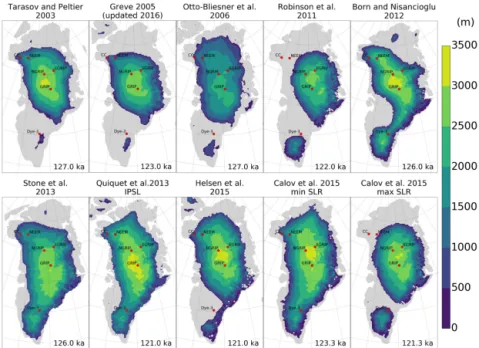
The SMB in most of the previous Eemian studies was cal-culated with an empirical PDD model. The exceptions are Robinson et al. (2011) and Calov et al. (2015), who used an intermediate complexity statistical downscaling with a lin-earized energy balance scheme to also include shortwave ra-diation. Furthermore, Helsen et al. (2013) used a full surface energy balance model (included in a RCM). Finally, Goelzer et al. (2016) employed a fully coupled (coarse resolution) GCM–ice sheet model to simulate the Eemian GrIS evolu-tion while employing a PDD model for the SMB calculaevolu-tion. A comparison of the minimum Eemian Greenland ice sheets from several studies is shown in Fig. 2. The estimated ice sheet extent and the volume loss (expressed as sea level rise contribution) vary strongly between the studies. All mod-els show large ice loss in the southwest, and several studies show a separation of the ice sheet into a northern and a south-ern dome. Additionally, some studies also exhibit extensive ice loss in the north, while this northern ice loss is absent in other studies. Overall, the estimated Eemian sea level rise contribution from Greenland remains uncertain due to the big differences between these studies. However, it is impor-tant to emphasize that the early studies partly lacked proxy data to constrain model results (i.e., ice core records), which were available to more recent studies. As an example, Otto-Bliesner et al. (2006) assumed an ice-free Dye-3 location during the Eemian as an evaluation criterion for their
sim-ulations. However, scientists now argue that there is indeed Eemian ice at the bottom of all deep ice core sites (Johnsen and Vinther, 2007; Willerslev et al., 2007).
3 Models and methods
3.1 Model description
We use the output of an Earth system model (ESM) and a RCM to assess the influence of the model resolution on the simulated SMB in Greenland. The regional model is forced with the global model output (i.e., the regional model is con-strained by the global model simulations at its boundaries). Furthermore, three different SMB models of various com-plexity are tested, forced with the global as well as the re-gional climates. Throughout this study, we refer to the two simulated climates as global (from the ESM) and regional (from the RCM).
Norwegian Earth System Model (NorESM)
The Norwegian Earth System Model (NorESM) was first in-troduced by Bentsen et al. (2013) and was included as ver-sion NorESM1-M in phase 5 of the Climate Model Inter-comparison Project (CMIP5; Taylor et al., 2011). NorESM is based on the Community Climate System Model ver-sion 4 (CCSM4; Gent et al., 2011) but was modified to include an isopycnic coordinate ocean general circulation model that originates from the Miami Isopycnic Coordi-nate Ocean Model (MICOM; Bleck et al., 1992), an atmo-sphere component with advanced chemistry–aerosol–cloud– radiation schemes known as the Oslo version of the Commu-nity Atmosphere Model (CAM4-Oslo; Kirkevåg et al., 2013) and the HAMburg Ocean Carbon Cycle (HAMOCC) model (Maier-Reimer, 1993; Maier-Reimer et al., 2005) adapted to the isopycnic ocean model framework.
In this work, we use a newly established variation of NorESM1-M, named NorESM1-F (Guo et al., 2018), that re-tains the resolution (2◦ atmosphere/land, 1◦ ocean/sea ice) and the overall quality of NorESM1-M but which is a computationally efficient configuration that is designed for multi-millennial and ensemble simulations. In NorESM1-F, the model complexity is reduced by replacing CAM4-Oslo with the standard prescribed aerosol chemistry of CAM4. The coupling frequency between atmosphere–sea ice and atmosphere–land is reduced from half-hourly to hourly, and the dynamic sub-cycling of the sea ice is reduced from 120 to 80 sub-cycles. These changes speed the model up by ∼ 30 %, while having a relatively small effect on the model’s over-all climate. In addition, some recent code developments for NorESM CMIP6 are implemented, as documented in detail by Guo et al. (2018). In particular, the updated ocean physics in NorESM1-F leads to improvements over NorESM1-M in the simulated strength of the Atlantic Meridional
Overturn-Figure 1.Overview of previously published GrIS contributions to the Eemian sea level high stand. The studies are color coded according to the atmospheric forcing used. More likely values are indicated with darker colors if provided in the respective studies. Different conversions from melted ice volume to sea level rise are used, and therefore the contributions are transformed to a common conversion if sufficient data (i.e., the pre-industrial ice volume for the respective simulations) are available. Due to this conversion, some of the values in this figure are slightly different from the original publications. We use a simple uniform distribution of the water volume on a spherical Earth. The common sea level rise conversion is performed for Greve (2005), Robinson et al. (2011), Born and Nisancioglu (2012), Quiquet et al. (2013), Helsen et al. (2013), and Calov et al. (2015). The minimum ice extent and topography of studies marked with “F2” are shown in Fig. 2.
ing Circulation and Arctic sea ice, both of which are impor-tant metrics when simulating past and future climates.
Positive degree day (PDD) model
The PDD method was introduced by Reeh (1989). The model is based on an empirical relationship between temperature and surface melt. Its minimum requirements are the monthly near-surface air temperature and the total precipitation. Due to its simplicity and low input requirements, it is often used in paleoclimate studies where the data availability is limited and the timescales of interest are long. Here, we use the PDD model as a legacy baseline with commonly used melt factors for snow and ice (e.g., Letréguilly et al., 1991; Ritz et al., 1997; Lhomme et al., 2005; Born and Nisancioglu, 2012).
The model integrates the number of days with tempera-tures above freezing into a PDD variable, which is multiplied by empirically based melt factors to calculate the amount of snow and ice melt. Different factors for snow and ice are ap-plied to account for the differences in albedo. The
tempera-ture variability during a month is simulated assuming a Gaus-sian distribution. The most important PDD model parameters are summarized in Table 1. Since a PDD model exclusively uses temperature to calculate melt, it only accounts for the terms in the surface energy balance which are directly related to temperature. It does not directly account for shortwave ra-diation; i.e., a PDD model is always tuned to present-day in-solation conditions. This is of particular relevance in studies of past climates, such as the Eemian, which exhibit different seasonal insolation patterns compared to today. Van de Berg et al. (2011) showed that a PDD model underestimates melt compared to a full SEB model when using PDD melt factors tuned to present-day conditions.
Here, we use a PDD model introduced by Seguinot (2013) and modify it to our needs. The PDD model uses the total monthly precipitation and calculates the snow fraction and accumulation via two threshold temperatures. If the temper-ature is below −10◦C, all precipitation falls as snow, and if the temperature is above 7◦C, all precipitation falls as rain and does not contribute to the accumulation. Between these
Figure 2.Overview of previously modeled minimum ice extent and topography of the Eemian GrIS. The number in the lower right corner of each panel refers to the timing of the minimum ice extent in the respective simulation. Deep ice core locations are indicated with red circles.
Table 1.Model parameters of the empirical PDD model. PDD model parameters
PDD snow melt factor 3 mm K−1day−1 PDD ice melt factor 8 mm K−1day−1 Maximum snow refreezing 60 % Maximum ice refreezing 0 % All snow temperature −10◦C All rain temperature 7◦C Standard deviation of the near- 4.5◦C surface temperature
extremes, a linear relation is applied to calculate the snow fraction.
BErgen Snow SImulator (BESSI)
The intermediate complexity SMB model, BErgen Snow SImulator (BESSI), is designed to be computationally effi-cient and to be forced by low-complexity climate models. It uses only daily mean values of three input fields: tempera-ture, precipitation, and downward shortwave radiation. Fur-thermore, outgoing longwave radiation is calculated prog-nostically, while incoming longwave radiation is calculated with a Stefan–Boltzmann law using the input near-surface air temperature and a globally constant air emissivity. BESSI is introduced in Imhof (2016) and Born et al. (2018). It is a physically consistent multi-layer SMB model with firn com-paction. The firn column is modeled on a mass-following, Lagrangian grid. BESSI uses a SEB that includes heat
dif-Table 2.Model parameters of the intermediate complexity BESSI model.
BESSI model parameters
Albedo dry snow 0.85
Albedo wet snow 0.70
Albedo ice 0.40
Bulk coefficient sensible heat flux 5.0 W m−2K−1
Air emissivity 0.87
Pore volume available to liquid water 0.1 Number of snow layers 15
fusion in the firn, retention of liquid water, and refreezing. However, it neglects sublimation which is of low impor-tance for the mass balance of Greenland. Firn densification is simulated with models commonly used in ice core research, following Herron and Langway (1980) for densities below 550 kg m−3 and Barnola et al. (1990) for densities above 550 kg m−3. There is no water routing on the surface, but the firn can hold up to 10 % of its pore volume in water. All excess water percolates into the next grid box below and if it reaches the bottom of the firn layer it is removed from the system. Table 2 summarizes the most important BESSI model parameters.
Modèle Atmosphérique Régional (MAR)
We use MAR to produce high-resolution SMB over the GrIS during the Eemian interglacial period. MAR is a regional atmospheric model fully coupled to the land surface model
SISVAT (Soil Ice Snow Vegetation Atmosphere Transfer) which includes a detailed snow energy balance model (Gal-lée and Duynkerke, 1997). The atmospheric part of MAR uses the solar radiation scheme of Morcrette et al. (2008) and accounts for the atmospheric hydrological cycle (including a cloud microphysical model) based on Lin et al. (1983) and Kessler (1969). The snow–ice part of MAR is derived from the snowpack model Crocus (Brun et al., 1992). This 1-D model simulates fluxes of mass and energy between snow layers, and reproduces snow grain properties and their effect on surface albedo.
The present work uses MAR version 3.6 in a similar model setup as in Le clec’h et al. (2017) with a fixed present-day ice sheet topography. We use a horizontal resolution of 25×25 km covering the Greenland domain (6600 grid points; stereographic oblique projection with its origin at 40◦W and 70.5◦N) from 60 to 20◦W and from 58 to 81◦N. The model has 24 atmospheric layers from the surface to an altitude of 16 km. SISVAT has 30 layers to represent the snowpack (with a depth of at least 20 m over the permanent ice area) and seven levels for the soil in the tundra area. The snowpack initialization is described in Fettweis et al. (2005).
MAR has often been validated against in situ observa-tions, e.g., in Fettweis (2007); Fettweis et al. (2013, 2017). Lateral boundary conditions can be provided either by re-analysis datasets (such as ERA-Interim or the National Cen-ters for Environmental Prediction – NCEP) to reconstruct the recent GrIS climate (1900–2015) (Fettweis et al., 2017) or by GCMs (e.g., Fettweis et al., 2013). In this study, the initial topography of the GrIS as well as the surface types (ocean, tundra, and permanent ice) are derived from Bam-ber et al. (2013). At its lateral boundaries, MAR is forced every 6 h with NorESM atmospheric fields (temperature, hu-midity, wind, and surface pressure) and at the ocean surface, NorESM sea surface temperature and NorESM sea ice ex-tent are prescribed. All needed NorESM output is bilinearly interpolated on the 25 × 25 km MAR grid.
For the SMB calculation, MAR assumes ice coverage af-ter all firn has melted. The calculated SMB is weighted by a ratio-of-glaciation mask derived from Bamber et al. (2013). For consistency, this mask is used for all PDD- and BESSI-derived SMBs as well. Regions with less than 50 % perma-nent ice cover are not considered for our analysis (similarly to Fettweis et al., 2017).
3.2 Experimental design, model spin-up, and terminology
Model experiment setup
We use five NorESM time slice simulations – a pre-industrial control run and four runs representing Eemian conditions at 130, 125, 120, and 115 ka, respectively. All five NorESM runs are dynamically downscaled with MAR; i.e., MAR is constrained with NorESM output at its boundaries. All
cli-mate simulations in this study use a static pre-industrial ice sheet. The output from all NorESM and MAR runs is used to force the different SMB models.
The NorESM pre-industrial experiment is spun up for 1000 years to reach a quasi-equilibrium state, followed by another model run of 1000 years representing the pre-industrial control simulation. The four Eemian time slice ex-periments (130, 125, 120, and 115 ka) are branched off af-ter the 1000-year spin-up experiment and run for another 1000 years each. The simulations are close to equilibrium at the end of the integration, with very small trends in, e.g., top-of-the-atmosphere radiation imbalance (0.02, 0.04, 0.02, and 0.02 W m−2 per century, respectively, between model years 1801 and 2000; all trends are statistically insignificant) and global mean ocean temperature (−0.008, −0.01, −0.03, and −0.03 K per century, respectively, between model years 1801 and 2000; all trends are statistically significant except for the 130 ka case). Statistical significance of the calculated trends is tested using the Student’s t test with the number of degrees of freedom, accounting for autocorrelation, calculated fol-lowing Bretherton et al. (1999). Trends with p values < 0.05 are considered to be statistically significant.
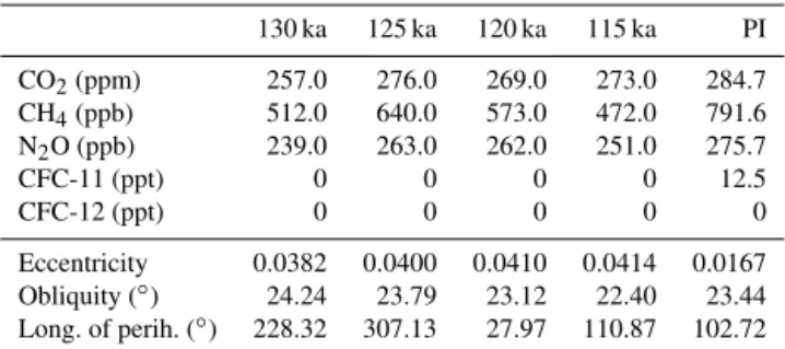
The model configurations follow the protocols of the third phase of the Paleoclimate Modelling Intercomparison Project (PMIP3). Compared with the experimental setup of the pre-industrial control simulation, only the orbital forcing and the greenhouse gas concentrations are changed in the four Eemian experiments. The greenhouse gas concentrations and the orbital parameters used are listed in Table 3.
For the MAR experiments, NorESM is run for another 30 years for each of the five experiments and the output is saved 6-hourly. These 30 years are used as boundary forcing for MAR. The first 4 years are disregarded as spin-up and the final 26 years are used for the analysis here.
BESSI is forced with daily fields of temperature, pre-cipitation, and downward shortwave radiation of these final 25 climate model years of NorESM and MAR, respectively. The forcing is applied cyclically (forwards and backwards) six times until SMB values reach an equilibrium. The SMBs of the final seventh cycle are used to calculate annual means over 25 years which are used in the analysis.
Experiment terminology
We force the PDD model with monthly near-surface air tem-perature and precipitation fields from NorESM and MAR, and refer to the resulting SMBs as NorESM-PDD and MAR-PDD, respectively. MAR has a full SEB model implemented and its derived SMB is referred to as MAR-SEB. Addi-tionally, we force the intermediate complexity SMB model, BESSI, with daily NorESM and MAR near-surface air tem-perature, precipitation, and the downward shortwave radia-tion, and call its output NorESM-BESSI and MAR-BESSI, respectively. An overview of the experimental design is shown in Fig. 3.
Table 3. Greenhouse gas concentrations and orbital parameters used for the NorESM and MAR climate simulations (PI: pre-industrial). 130 ka 125 ka 120 ka 115 ka PI CO2(ppm) 257.0 276.0 269.0 273.0 284.7 CH4(ppb) 512.0 640.0 573.0 472.0 791.6 N2O (ppb) 239.0 263.0 262.0 251.0 275.7 CFC-11 (ppt) 0 0 0 0 12.5 CFC-12 (ppt) 0 0 0 0 0 Eccentricity 0.0382 0.0400 0.0410 0.0414 0.0167 Obliquity (◦) 24.24 23.79 23.12 22.40 23.44 Long. of perih. (◦) 228.32 307.13 27.97 110.87 102.72
For lack of observational data with a comprehensive cov-erage, we use the most complex model, MAR-SEB, as our reference SMB model. The standard PDD experimental setup (see Table 1) is tuned to present-day Greenland. The interme-diate complexity SMB model, BESSI, is tuned to the MAR-SEB under pre-industrial conditions in terms of SMB and refreezing. The first tuning goal is the total integrated SMB within ±50 Gt and the smallest possible root mean square (rms) error. From the set of model parameters which fulfill this goal, we choose the set which shows the best fit to re-freezing (total amount and rms error). The most important model parameters for the empirical PDD and the intermedi-ate SMB model, BESSI, are summarized in Tables 1 and 2, respectively.
We compare the five SMB model experiments (NorESM-PDD, MAR-(NorESM-PDD, NorESM-BESSI, MAR-BESSI, and MAR-SEB) under pre-industrial conditions and analyze the evolution of their respective SMB components during the Eemian interglacial period.
Interpolation of temperature fields to a higher-resolution grid
To derive realistic near-surface air temperatures on a higher-than-climate-model resolution (e.g., an ice sheet model grid but also from the NorESM to the MAR grid), it is neces-sary to account for the coarser topography in the initial cli-mate model. In this study, the NorESM temperature is bilin-early interpolated on the MAR grid and a temperature lapse rate correction is applied to account for the height difference caused by the different resolutions.
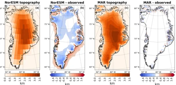
The model topographies of Greenland in NorESM and MAR are shown in Fig. 4a and c. Both represent the present-day ice sheet but in different spatial resolutions. The differ-ence with the observed, high-resolution topography (Schaffer et al., 2016) is also shown in Fig. 4b and d. Due to the lower spatial resolution of NorESM and the resulting smoothed model topography, differences between model and observa-tions are large and cover extensive areas. On the contrary, the differences for the MAR topography to observations are lo-calized at the margins of the ice sheet and much smaller. The
strong resemblance of the MAR topography and the obser-vations allows us to use the MAR temperature directly, with-out any correction. Furthermore, we perform a sensitivity test for PDD-derived SMB comparing various temperature lapse rates and discuss its results in Sect. 4.2.
4 Pre-industrial simulation results
4.1 Pre-industrial climate
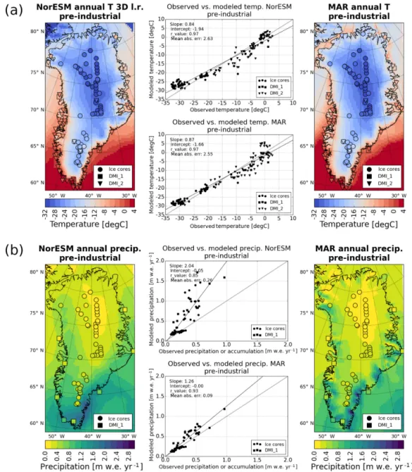
The pre-industrial annual mean NorESM and MAR near-surface air temperatures are compared with the observations in Fig. 5a. The observations are taken from a collection of shallow ice core records and coastal weather station data compiled by Faber (2016). The data cover the time period from 1890 to 2014. However, individual stations cover only parts of this period. DMI_1 stations provide annual mean temperature and precipitation, whereas DMI_2 stations only provide temperature. The NorESM temperature is bilinearly interpolated to the MAR grid and corrected to the MAR to-pography with a model consistent, temporally and spatially varying lapse rate derived from NorESM; i.e, we use the lapse rate of the NorESM atmosphere above each grid cell. Sensitivity experiments with various lapse rates are discussed in Sect. 4.2. Due to the lack of observations, we are not com-paring the exact same period here, resulting in an inherent offset between climate model and observations.
The NorESM and MAR temperatures agree well with the observations from the coastal regions. However, MAR simu-lates warmer temperatures than NorESM at the northern rim of Greenland, an area which is underrepresented in the ob-servations. The cold temperatures in the interior are better captured by MAR than by NorESM.
The annual mean NorESM and MAR precipitation, un-der pre-industrial conditions, is shown in Fig. 5b. Compared to the observations, both climate models overestimate pre-cipitation. This overestimation is visible due to the fact that most scatter points are above the gray 1 : 1 diagonal, indicat-ing a too-high model value. However, it is important to note that observations from ice cores represent accumulation (i.e., precipitation minus snow drift, sublimation, and similar pro-cesses) rather than precipitation, which partly explains the overestimation at the ice core locations. In general, the MAR precipitation shows less spread and is closer to the obser-vations than NorESM. The precipitation pattern of NorESM is related to its coarse representation of Greenland’s topog-raphy. On the other hand, MAR with its finer resolution re-solves coastal and local maxima. Unfortunately, the locations with the highest precipitation rates are not covered by the ob-servations.
Figure 3.Overview of the experimental design. The simple PDD and intermediate BESSI SMB simulations are forced with output of our global climate (from NorESM) and the regional climate (from MAR). Additionally SMB is derived from the SEB model implemented in MAR. This flow of experiments is performed in the same way for all five time slices (130, 125, 120, 115 ka, and pre-industrial).
Figure 4.Greenland model topographies and differences to observed Greenland topography from Schaffer et al. (2016). (a) NorESM Green-land topography, on the original resolution of 1.9 × 2.5◦(latitude/longitude), (b) NorESM minus observed, (c) MAR Greenland topography (on original resolution of 25 × 25 km), and (d) MAR minus observed.
4.2 Sensitivity of PDD-derived SMB to temperature lapse rate correction
For a consistent comparison of the NorESM and MAR tem-peratures, calculated on different model grids, a temperature lapse rate correction is applied to the NorESM temperatures to account for the elevation difference of the model surfaces. Previous studies often use spatially uniform values between 5◦C km−1 (e.g., Abe-Ouchi et al., 2007; Fyke et al., 2011) and close to 8◦C km−1(e.g., Huybrechts, 2002). Temporally varying temperature lapse rates are used by Quiquet et al. (2013) and Stone et al. (2013). We use 6.5◦C km−1as our default lapse rate (e.g., Born and Nisancioglu, 2012). How-ever, we test spatially and temporally uniform lapse rates be-tween 5 and 10◦C km−1. Additionally, we derive the lapse rate of the free troposphere from the NorESM vertical atmo-spheric air column above each grid cell (i.e., minimum lapse rate above the surface inversion layer). We refer to this as the 3-D lapse rate. Furthermore, we calculate the moist adi-abatic lapse rate (MALR; American Meteorological Society, 2018) from the thermodynamic state of the NorESM surface air layer via pressure, humidity, and temperature. The MALR
is the rate of temperature decrease with height along a moist adiabat. Both the 3-D lapse rate as well as the MALR vary in time and space.
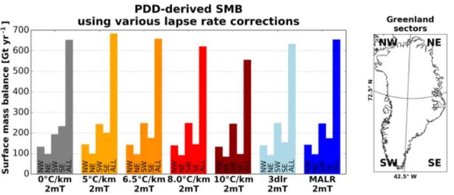
The integrated PDD-derived SMB in Greenland, using these different lapse rates, is compared in Fig. 6. Greenland is split into four sectors along 72.5◦N and 42.5◦W to inves-tigate regional differences. Focusing on the temporally and spatially uniform lapse rates shown in red colors reveals little effects on the PDD-derived SMB, except in the SE – higher lapse rates give lower SMB in southeast Greenland. The ex-tremely high lapse rate of 10◦C km−1 shows the strongest reduction in SMB. For the uncorrected temperature fields of NorESM (gray columns), the relative contribution of the southeast (SE) and southwest (SW) sectors of Greenland are switched, giving a larger SMB contribution from SE Green-land. In this uncorrected case, ablation is almost completely absent in the SE sector, even in the lowest coastal regions (not shown), which is not realistic (compare our reference MAR-SEB results in Fig. 7e). Furthermore, the SMB in the SW is much more negative than our reference MAR-SEB results.
Figure 5.Annual mean near-surface air temperature and precipitation simulated with NorESM and MAR for pre-industrial conditions. The NorESM temperature is corrected with the temporally and spatially varying 3-D lapse rate (see Sect. 4.2). Row (a) shows modeled temperatures with observations from ice cores and weather stations plotted on top. Additionally, scatter plots of observed vs. modeled temperature for each model are presented. The bold gray lines represent the 1 : 1 diagonal and hence a perfect fit between model and observations. Row (b) shows the same for annual mean precipitation.
The general pattern for the PDD-derived SMBs, calculated using a uniform temperature lapse rate, is that the SMB is reduced as the lapse rate increases, mainly due to the de-crease in SMB in SE Greenland. This might seem counter intuitive, since most of the NorESM topography is lower than observations (blue colors in Fig. 4). However, a closer look at Fig. 4 reveals that large parts of the margins are higher than observations (red colors) which results in a warming when applying the lapse rate correction. Additionally, the margins
are also the major melt regions. Therefore, higher lapse rates lead to warmer margins, and as a result, to a lower SMB.
The 3-D lapse rate as well as the MALR correction (blue colors) result in total and regional SMBs between those which follow from using the uniform lapse rates of 6.5 and 8◦C km−1. This makes sense since the mean values of the 3-D lapse rate and MALR are close to 6.5 and 8◦C km−1, respectively. In general, the total SMB as well as the spa-tial pattern of the SMB in Greenland (not shown) is similar to all the lapse rate corrections. A different SMB pattern is
Figure 6.Sensitivity of the PDD-derived SMB to the applied temperature lapse rate correction (to low-resolution climate). The bars show the integrated SMB over the GrIS and its regional contributions. 0◦C km−1refers to the uncorrected temperature, 5 to 10◦C km−1represent spatially uniform temperature lapse rates, 3dlr is the 3-D lapse rate derived from the vertical NorESM temperature column, and MALR is the moist adiabatic lapse rate calculated from the thermodynamic state of the NorESM surface air layer.
only seen when employing the uncorrected temperatures – the contributions from the SE and SW are switched; i.e., there is more extensive melt in the SW and less in the SE because the coastal small-scale features are absent in the uncorrected NorESM temperature due to its relatively coarse resolution.
We conclude that it is necessary to apply a temperature lapse rate correction to lower-resolution temperature fields to obtain a realistic spatial SMB pattern, because using GCM temperature directly in a PDD model results in a coarse rep-resentation of the SMB – a wide ablation zone in the west and virtually no ablation on the east coast (not shown). However, the exact value of the lapse rate is less important when using a PDD model. For the comparison of NorESM temperature and observations in Fig. 5a, we use the model consistent 3-D lapse rate.
The influence of the lapse rate correction on the PDD-derived SMB is minimal and the results from the 3-D lapse rate and the uniform 6.5◦C km−1(which was used before) are very similar; therefore, we use the latter in our PDD cal-culations. We do not aim to adapt PDD in this study but rather use it as a legacy baseline. The correction is applied to NorESM-PDD and NorESM-BESSI. MAR temperature is not corrected, since the MAR topography represents obser-vations sufficiently well (see Fig. 4).
4.3 Pre-industrial surface mass balance
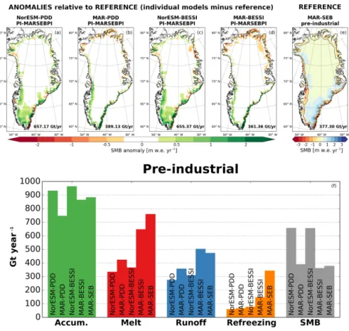
The simulated pre-industrial SMBs from all five model com-binations are shown in Fig. 7. Figure 7e shows our reference, MAR-SEB, which we compare all model experiments to. Both derived SMBs, PDD and NorESM-BESSI (Fig. 7a and c), show a stronger and spatially more extensive positive SMB anomaly compared to the other ex-periments. The accumulation in the south looks similar to the NorESM precipitation pattern in Fig. 5b, which leads to this positive SMB anomaly. Since NorESM is unable to re-solve the narrow precipitation band in the southeast correctly, the accumulation is spread out over a larger region reaching
further inland. The narrow ablation zone in the southeast (as simulated by MAR-SEB), is much less pronounced in all four simpler model experiments. Similar to the NorESM-derived SMBs, MAR-PDD and MAR-BESSI (Fig. 7b and d) also show a positive SMB anomaly on the margins but not in the southern interior.
Figure 7f shows the Greenland-integrated SMB compo-nents. All models are compared on a common ice mask (i.e., less than 50 % permanent ice cover in MAR; see Sect. 3.1). The NorESM-forced experiments, NorESM-PDD and NorESM-BESSI, show the higher total integrated SMBs (gray bars) as a result of the high accumulation (green bars) and low melt (red bars). Both are related to the lower reso-lution of NorESM (i.e., the narrow precipitation band in the southeast is not captured and the precipitation is smoothed over the whole southern tip of Greenland). Furthermore, the lower resolution of NorESM causes its ice mask to reach be-yond the common MAR ice mask (not shown) and poten-tial NorESM ablation regions are partly cut off. The forced experiments, PDD, BESSI, and MAR-SEB, show better agreement with each other, but the simpler models underestimate melt and refreezing. This is generally true for the four simpler models. In particular, the refreezing values are much lower than in our reference, MAR-SEB. It is not surprising that the PDD model does not capture ing as it uses a very simple parameterization (i.e., the refreez-ing is limited to 60 % of the monthly accumulation; follow-ing Reeh, 1989). The intermediate model, BESSI, has a firn model implemented (see Sect. 3.1) but also shows much less refreezing than our reference, MAR-SEB.
5 Eemian simulation results
5.1 NorESM Eemian simulations
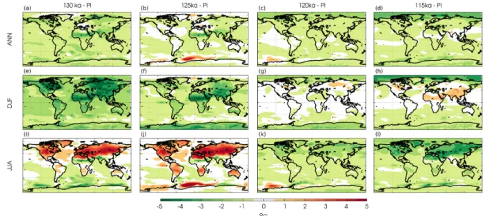
Simulated changes of annual mean, boreal winter (December–January–February; DJF), and boreal sum-mer (June–July–August; JJA) near-surface air temperatures
Figure 7.Comparison of the simulated pre-industrial SMB from all five model setups. The first row shows the spatial map of SMB for NorESM-PDD, MAR-PDD, NorESM-BESSI, MAR-BESSI, and MAR-SEB, respectively. Our reference, MAR-SEB (e), is shown in ab-solute values, while the four simpler models (a–d) are shown as anomalies to MAR-SEB. The total SMB integrated over all of Greenland (including grid cells with more than 50 % permanent ice) is given in numbers on each panel. The same ice mask is used for the bar plots (f). The bar plots show the individual components contributing to the total SMB (in Gt yr−1) for each model.
for the four Eemian time slices are shown in Fig. 8. Annual mean temperature changes are relatively small compared to the seasonal changes due to the strong seasonal insolation anomalies during the Eemian interglacial period. However, there was a total annual irradiation surplus at high latitudes during the Eemian (Past Interglacials Working Group of PAGES, 2016, Fig. 5d therein), and analysis of proxy data has revealed with high confidence that high-latitude surface temperature, averaged over several thousand years, was at least 2◦C warmer than present during the Eemian (Masson-Delmotte et al., 2013). The annual warming signal at high latitudes is not as pronounced in the NorESM simulations. However, a strong summer warming is simulated over the Northern Hemisphere, which is particularly important for the Eemian melt season and therefore Greenland’s SMB. Especially during the early Eemian (130/125 ka), a strong seasonality is simulated globally, with extensive DJF cooling and JJA warming in general on the Northern Hemisphere landmass. In the Southern Ocean, near-surface temperatures are cooler/warmer at 130/125 ka than the pre-industrial climate, respectively, with the former associated with an ice-free Weddell Sea in austral winter. Arctic warming is
ab-sent or not pronounced in both seasons in the early Eemian. The seasonal changes of near-surface temperature during the late Eemian (120/115 ka) are more modest compared to the early Eemian. During DJF, high-latitude cooling is simulated in both hemispheres, with enhanced warming in most of the Northern Hemisphere subtropical land region at 115 ka. During JJA, an overall hemisphere-asymmetric cooling pattern is simulated, with especially enhanced cooling simulated in the Northern Hemisphere land region at 115 ka.
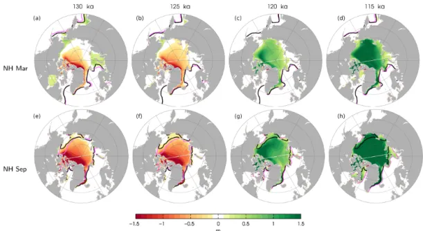
Simulated anomalies of Arctic sea ice concentrations and thicknesses during the four Eemian time slices (Fig. 9) largely reflect the changes of surface temperature in this re-gion. During the early Eemian, the March sea ice extent is close to the pre-industrial distribution, with thinner ice near the central Arctic, around the coast of Greenland, and the Canadian Archipelago. The September sea ice has a smaller extent on the Pacific side of the Arctic, with even thinner sea ice across the whole Arctic, especially north of Greenland and the Canadian Archipelago (> 1.5 m ice thickness reduc-tion). During the late Eemian, the March sea ice extent is also similar to the pre-industrial simulation, whereas the
Septem-Figure 8. Simulated changes of near-surface air temperature for the Eemian experiments relative to the pre-industrial experiment (PI). Panels (a)–(d) show the annual mean, and panels (e)–(h) and (i)–(l) show the DJF and JJA mean, respectively. The columns show the temperature changes for the 130, 125, 120, and 115 ka experiments from left to right. Model results are annual means over the last 100 years of model integration. A latitude/longitude grid is indicated with dashed lines with a 60◦spacing.
ber sea ice extent is larger on the Pacific side of the Arctic. The sea ice is thicker in both seasons, especially for 115 ka. The ice thickness increase is greater than 1.5 m in the cen-tral Arctic in March and almost across the whole Arctic in September.
5.2 Eemian Greenland climate
The evolution of the simulated Eemian Greenland mean JJA temperature is shown in Fig. 10. As temperature during the melt season strongly influences the SMB, JJA temperature is a good indicator for the evolution of the SMB. The 125 ka time slice is the warmest for both climate models. While NorESM (Fig. 10a) shows a maximum summer warming of up to 3◦C in the interior, MAR anomalies (Fig. 10b) reach up to 5◦C at 125 ka. During the two earliest and warmest Eemian time slices, 130 and 125 ka, MAR shows particular warm and localized anomalies on the eastern and northeast-ern coasts. The locations of these anomalies overlap with MAR regions without permanent ice cover. This localized warm anomaly is absent in NorESM. The later Eemian time slices, 120 and 115 ka, are both cooler than the pre-industrial. The evolution of the simulated Eemian precipitation rela-tive to the simulated pre-industrial precipitation is shown in Fig. 11. The warmest periods of the Eemian, 130 and 125 ka, show more precipitation in the northwest. In particular, MAR shows a positive anomaly of up to 50 % in this region at 125 ka. The coldest Eemian period, 115 ka, shows a small de-crease of 10 %–20 % in precipitation for large parts of Green-land and 120 ka shows the smallest anomalies of all the time slices. Overall, NorESM and MAR show the same
precipita-tion trends, but the MAR changes are more pronounced and show stronger regional differences which can be attributed to the higher resolution of MAR compared to NorESM.
5.3 Eemian surface mass balance
The MAR-SEB simulation is also our SMB reference for the Eemian. The 130 ka MAR-SEB (Fig. 12e) shows a relative uniform reduction in SMB all around the Greenland margins (cf., the MAR-SEB pre-industrial run; Fig. 7e). The strongest reduction can be seen in the southwest, where the main ab-lation zone is located (similar to pre-industrial). However, there is also a noteworthy SMB reduction in the northeast. The comparison of the other four SMB models at 130 ka rel-ative to the 130 ka MAR-SEB reference is given in Fig. 12a to d. The 130 ka results are shown here in detail since all model experiments show their respective lowest SMBs for this time slice; i.e., they represent our most extreme Eemian SMBs, in spite of 125 ka showing higher summer tempera-tures (see Fig. 10) than 130 ka. This is related to the stronger positive insolation anomaly in spring at 130 ka compared to 125 ka (not shown), giving a prolonged melt season early in the Eemian. Under 130 ka conditions, there are 60 days with a daily mean shortwave insolation above 275 W m−2, in con-trast to 54 days at 125 ka and only 19 for pre-industrial condi-tions (calculated between 58 and 70◦N in the MAR domain). In regions between 40 and 70◦N, an insolation threshold of 275 W m−2is an indicator for temperatures close to the freez-ing point (Huybers, 2006).
Figure 9.Simulated changes of Arctic sea ice thickness for the four Eemian experiments relative to the pre-industrial experiment. Panels (a)– (d) and (e)–(h) show the sea ice changes in March and September, respectively. The columns show the sea ice changes for the 130, 125, 120, and 115 ka experiments from left to right. The solid magenta and black contour lines show the 15 % sea ice concentration for each Eemian experiment and the pre-industrial experiment, respectively. Model results are annual means from the last 100 years of model integration. A latitude/longitude grid is indicated with gray lines with a 10/60◦spacing.
The NorESM-forced SMB models, NorESM-PDD and NorESM-BESSI (Fig. 12a and c), show a more positive SMB anomaly at the southern tip of Greenland, which is in con-trast to all other model experiments. This NorESM-specific feature corresponds to a less negative SMB in the ablation zone at the margins and a more positive SMB in the inte-rior accumulation zone relative to MAR-SEB. The coarser resolution of NorESM causes accumulation to be smoothed over the whole southern domain, instead of being local-ized to the southeast margin, where the highest accumula-tion rates are reached in the higher-resoluaccumula-tion MAR-forced experiments (Fig. 12b and d). Due to this resolution effect, also the total integrated SMB of the NorESM-forced experi-ments is higher than the MAR-forced experiexperi-ments. However, NorESM-BESSI (Fig. 12c) shows a lower SMB in the north-east than MAR-SEB, which causes its total SMB to be less positive than NorESM-PDD.
From the MAR-forced experiments, MAR-PDD (Fig. 12b) shows a similar spatial SMB pattern as NorESM-PDD. How-ever, MAR-PDD shows more ablation in the north than NorESM-PDD and there is also no resolution-related accu-mulation surplus in the south. The higher integrated SMB compared to the MAR-SEB reference is therefore mostly re-lated to less ablation. Since MAR-SEB and MAR-PDD are forced with the same temperature and precipitation fields, it can be concluded that the missing ablation in MAR-PDD is caused by neglecting shortwave radiation in the PDD model. MAR-BESSI (Fig. 12d) shows a lower SMB further inland
including large areas in the north. This is a feature of both BESSI experiments but less pronounced in NorESM-BESSI. The integrated SMB (gray bars; Fig. 12f) of MAR-BESSI fits MAR-SEB best; however, the spatial SMB pattern is dif-ferent. A common ice mask is applied, i.e., more than 50 % permanent ice cover in MAR. MAR-BESSI has less ablation around the margins, but the lower ablation is more than com-pensated by stronger melt in the north, resulting in a SMB more than 100 Gt yr−1 lower compared to MAR-SEB. The accumulation (green bars; Fig. 12f) remains relatively un-changed compared to pre-industrial simulations (Fig. 7f) – the total amount as well as the difference between the indi-vidual SMB experiments. The NorESM-forced experiments show slightly higher accumulation, while MAR-PDD shows the lowest accumulation. The accumulation differences be-tween PDD and BESSI are a result of the different snow/rain threshold temperatures in PDD and BESSI, which are nec-essary due to different model time steps. NorESM-PDD is less affected because the NorESM temperature is lower in all time slices compared to MAR (Fig. 10). The melt (red bars; Fig. 12f) is a factor of 2 larger for all experiments com-pared to their respective pre-industrial experiments. MAR-SEB shows the highest melt, followed by MAR-BESSI. The three other models show much less melt.
Note that the amount of refreezing is doubled for most model experiments compared to pre-industrial conditions. MAR-SEB shows the largest amount of refreezing, fol-lowed by the BESSI experiments with around one-third of the MAR-SEB refreezing. The PDD models come last
Figure 10.Evolution of the simulated summer temperature (June–July–August; JJA) over Greenland during the Eemian interglacial period. NorESM temperatures (lapse rate corrected; see Sect. 3.2) are shown in row (a) and MAR temperatures in row (b). The Eemian temperatures are shown as anomalies relative to the pre-industrial simulation. The solid gray line indicates the 0◦C isotherm.
with around one-sixth of the MAR-SEB refreezing. Inter-estingly, NorESM-BESSI and MAR-BESSI show very sim-ilar refreezing at 130 ka, whereas the difference under pre-industrial conditions (Fig. 7f) is much more pronounced.
The integrated SMB at 130 ka is negative for MAR-SEB and MAR-BESSI, while the simpler models show posi-tive SMBs. Similar to the pre-industrial experiments, the NorESM-forced experiments are most positive, related to their coarse climate resolution (i.e., coarse accumulation rep-resentation, common ice mask cuts off NorESM ablation zones; see discussion in Sect. 4.2).
Finally, an overview of the Greenland-integrated SMB components for all model setups and time slices is shown in Fig. 13. The accumulation (Fig. 13a) shows a slight increase in warmer periods (130, 125 ka) for all experiments. There is a clear distinction between experiments using the PDD and BESSI models: the PDD models show lower values than their respective BESSI models (NorESM-PDD vs. NorESM-PDD and MAR-PDD vs. MAR-BESSI). This is related to the dif-ferent temporal forcing (PDD: monthly; BESSI: daily) and different snow/rain temperature thresholds (see Sect. 3.1). The relatively high values of the NorESM-forced
experi-ments are caused by the lower resolution of NorESM (see discussion in Sect. 4.2).
Melt (Fig. 13b) and runoff (Fig. 13d) are highest in the warm early Eemian. All 130 ka experiments show more melt and runoff than the 125 ka experiments, which is caused by the prolonged melt season at 130 ka; discussed earlier in this section. The refreezing (Fig. 13c), which is basi-cally the difference between melt and runoff, is much higher in MAR-SEB than in all other experiments: approximately one-third of the meltwater refreezes during the warm early Eemian time slices, and around one-half refreezes during the following colder periods. The other experiments show only a fraction of this refreezing. However, the BESSI ex-periments show slightly higher values than the PDD experi-ments. The spatial pattern of refreezing (not shown) is similar between MAR-SEB and MAR-BESSI during colder times slices (120, 115 ka, and pre-industrial) but very different dur-ing the warmer Eemian time slices (130 and 125 ka). The MAR-SEB refreezing pattern remains similar for all time slices, with an intensification around the margins, but par-ticularly in the south of Greenland, in the warmer Eemian time slices. In contrast, most MAR-BESSI refreezing during the two warm time slices occurs along the southeastern and
Figure 11.Evolution of the simulated annual precipitation during the Eemian interglacial period. NorESM precipitation is shown in row (a) and MAR precipitation in row (b). Eemian time slices are shown as anomalies relative to the pre-industrial simulation.
northeastern margins. The MAR-BESSI experiments in gen-eral show smaller refreezing quantities, while also increasing in the two warm time slices.
The integrated SMB (Fig. 13e) shows a clear differ-ence between and MAR-forced models. NorESM-forced models are offset towards positive values due to higher accumulation and less melt. The SMB of the MAR-BESSI experiment is consistent with MAR-SEB for all time slices. MAR-PDD is consistent with MAR-SEB for the cold time slices (120, 115, and pre-industrial) but is unable to cap-ture the negative SMBs at 130 and 125 ka.
6 Discussion
The Eemian interglacial period is characterized by a posi-tive Northern Hemisphere summer insolation anomaly giv-ing warmer summers in Greenland. This complicates PDD-derived Eemian SMB estimates since insolation is not in-cluded in PDD models. Here, we assess how the climate forc-ing resolution and the SMB model choice influences Eemian SMB estimates in Greenland. A Eemian global climate sim-ulation (with NorESM) is combined with regional dynami-cal downsdynami-caling (with MAR). Previous studies, using down-scaled SMB in Greenland, use either low-complexity models (Robinson et al., 2011; Calov et al., 2015) or climate
forc-ing from low-resolution global climate models (Helsen et al., 2013) as input. Unfortunately, the uncertainties associated with the global climate simulations add a major constraint to any high-resolution Greenland SMB estimate. For exam-ple, Eemian global climate model spread has been hypothe-sized to be related to differences in the simulated Eemian sea ice cover (Merz et al., 2016). Furthermore, sensitivity experi-ments with global climate models by Merz et al. (2016) show that sea ice cover in the Nordic Seas is crucial for Greenland temperatures (i.e., a substantial reduction in sea ice cover is necessary to simulate warmer Eemian Greenland tempera-tures in agreement with ice core proxy data). However, the quantification of Eemian global climate simulation uncer-tainties is beyond the scope of this paper and we refer the reader to Earth system model intercomparisons focusing on the Eemian (Lunt et al., 2013; Bakker et al., 2013), as well as studies seeking to merge data and models (e.g., Buizert et al., 2018), for details on efforts to improve Eemian climate estimates and reduce global climate uncertainties.
The Eemian climate simulations, with NorESM and MAR, are steady-state simulations with a fixed present-day topog-raphy of Greenland, neglecting any topogtopog-raphy changes or freshwater forcing from a melting ice sheet. Given the lack of a reliable Eemian Greenland topography or meltwater es-timate, this is a shortcoming we choose to accept. Merz et al.
Figure 12.Comparison of the simulated 130 ka SMB relative to the 130 ka MAR-SEB with all five model combinations. The first row shows the spatial map of SMB for NorESM-PDD (a), MAR-PDD (b), NorESM-BESSI (c), MAR-BESSI (d), and MAR-SEB (e), respectively. Our reference, MAR-SEB, is shown in absolute values, while the four simpler models (a–d) are shown as anomalies to MAR-SEB. The total SMB is integrated over all of Greenland (including grid cells with more than 50 % permanent ice). The same mask is used for the bar plots (f). The bar plots show the absolute values for each component of the SMB for the same experiments.
(2014a) discuss global climate steady-state simulations us-ing various reduced Eemian Greenland topographies without finding any major changes of the large-scale climate pattern. However, there is a clear impact of Greenland topography changes on the local near-surface air temperature, given that the surface energy balance is strongly dependent on the lo-cal topography (e.g., due to changes in lolo-cal wind patterns and surface albedo changes as a region becomes deglaciated). The same is true for the relationship between Greenland’s topography and Eemian precipitation patterns (Merz et al., 2014b) – large-scale patterns are fairly independent of the topography, but local orographic precipitation follows the slopes of the ice sheet. The impact of orographic precipita-tion is also clear when transiprecipita-tioning from low to high reso-lution in models: as an example, for the pre-industrial sim-ulation with MAR (comparing Fig. 11a and b), the higher-resolution topography results in enhanced precipitation along the better resolved sloping margins of the GrIS (e.g., the southeast margin).
Furthermore, Ridley et al. (2005) find an additional sur-face warming in Greenland in transient coupled 4xCO2 ice sheet–GCM simulations compared to uncoupled
simu-lations caused by an albedo–temperature feedback. Simi-larly, Robinson and Goelzer (2014) show that 30 % of the additional insolation-induced Eemian melt is caused by the albedo–melt feedback. Somewhat unexpectedly, given the higher temperatures, Ridley et al. (2005) find more melting in standalone ice sheet simulations than in the coupled simu-lations. The local climate change in the coupled runs results in a negative feedback that likely causes reduced melting and enhanced precipitation. They propose the formation of a con-vection cell over the newly ice-free margins in summer which causes air to rise at the margins and descend over the high-elevation ice sheet (too cold for increased ablation). This leads to stronger katabatic winds which cool the lower re-gions and prevent warm air from penetrating towards the ice sheet. An increased strength of katabatic winds can also be caused by steeper ice sheet slopes (Gallée and Pettré, 1998; Le clec’h et al., 2017).
At 130 ka, the GrIS was likely larger than today, as the cli-mate was transitioning from a glacial to an interglacial state. A smaller-sized ice sheet leads to higher simulated temper-atures in Greenland due to the lower altitude of the surface and the albedo feedback in non-glaciated regions.
Addition-Figure 13.Eemian evolution of the SMB components (integrated over grid cells with more than 50 % ice cover in MAR; Gt yr−1). Pre-industrial values for each model are shown as shaded lines in the background and as triangles on the side.
ally, neglecting the meltwater influx to the ocean from the retreating glacial ice sheet gives warmer simulated temper-atures (the light meltwater would form a fresh surface layer on the ocean and isolate the warm subsurface water from the atmosphere). As a result, the simulated 130 ka temperatures are likely warmer than the actual temperatures, resulting in a lower simulated SMB. Similarly, the present-day ice sheet, and particularly the ice mask, is likely misrepresenting the 125 ka state of Greenland. A larger ice sheet will include re-gions of potentially highly negative SMB, lowering the inte-grated SMB; i.e., the simulated inteinte-grated 125 ka SMBs are likely also too low to be realistic. Only a fully coupled ice sheet–atmosphere–ocean simulation would be able to
realis-tically account for evolving ice sheet configuration and melt-water input to the ocean. Here, the simulated 130 ka SMB is discussed in more detail, not because it is assumed to be the most realistic but because it provides the most extreme SMB cases within our Eemian climate simulations. Further-more, the spatial SMB pattern does not change significantly between 130 and 125 ka in our simulations; i.e., conclusions drawn for 130 ka are also true for 125 ka.
The comparison of different SMB models requires a com-mon ice sheet mask which is always a compromise. Vernon et al. (2013) show that approximately a third of the inter-model SMB variation between four different regional climate models is due to ice mask variations at low altitude (mod-els forced with 1960–2008 reanalysis data over Greenland). Resolution-dependent ice sheet mask differences between NorESM- and MAR-derived SMBs are important here. Due to the larger NorESM grid cells, the NorESM ice mask ex-tends beyond the common MAR ice mask (not shown), and as a result, the NorESM ablation zone is partly cut off when using the common MAR ice mask. As a consequence, there is less ablation in the NorESM-forced SMB model experiments than in the MAR-forced experiments. The direct compari-son between NorESM- and MAR-derived SMBs is therefore challenging. However, the PDD and BESSI models are run with both climate forcing resolutions to allow a consistent comparison, independent of the ice mask.
The results discussed in Sect. 5.3, particularly the differ-ences in melt during the warmer Eemian time slices, indicate two things. Firstly, it is problematic not to include shortwave radiation in a SMB model when investigating the Eemian, because the melt might be underestimated. Secondly, a SMB model cannot fix shortcomings of a global climate forcing (i.e., low resolution like here). Both the climate and the type of SMB are important for an accurate simulation of Green-land’s SMB, while either of the two can be more important depending on the climate state and particularly the prevailing insolation pattern.
For the cooler climate states (i.e., 120, 115 ka, and pre-industrial), the different climate forcing resolution shows the largest influences on the SMBs. The complexity and physics of the SMB model are of secondary importance during these periods. This comes as no surprise, as the PDD parame-ters employed are based on modern observations, and the intermediate model, BESSI, was tuned to represent MAR-SEB under pre-industrial conditions. As discussed earlier, the resolution-dependent difference is caused by higher accumu-lation in the south but also less abaccumu-lation due to the differences in the ice sheet masks.
In the warmer climate states (i.e., 130 and 125 ka), the complexity of the SMB model becomes the dominant factor for the SMBs. SMB model experiments including solar inso-lation and forced with the high-resolution climate show inte-grated Eemian SMBs which are negative. Testing the SMB models with two climate forcing resolutions illustrates the necessity to resolve local climate features – an inaccurate
cli-mate (e.g., due to coarse topography) will result in an inaccu-rate SMB. Besides coarse representation of Greenland’s to-pography, changes in ice sheet topography and sea ice cover are likely to have a major impact on the climate over Green-land during the Eemian. However, as mentioned above, it is beyond the scope of this study to evaluate the uncertainty in the simulated Eemian climate forcing.
Melt and refreezing show the biggest differences of the SMB components (runoff is basically the difference of these two) between individual models as well as between the time slices. The PDD-derived experiments lack melting compared to the other experiments, due to the neglected insolation. MAR-PDD shows slightly more melt partly because it uses the higher-resolution climate (i.e., a climate derived with bet-ter representation of surface processes and surface albedo). NorESM-PDD and MAR-PDD show the least refreezing, re-lated to the simple refreezing parameterization but also due to the smaller amount of melt. The intermediate model, BESSI, shows more melt in the warm Eemian and almost matches the values of the MAR-SEB reference experiments if forced with the regional climate. However, BESSI cannot compen-sate for the shortcomings of the lower-resolution climate in NorESM-BESSI. In general, BESSI shows slightly more re-freezing than PDD, but rere-freezing remains underrepresented compared to MAR-SEB. This is likely related to a fairly crude representation of the changing albedo (i.e., albedo is changed with a step function from dry to wet snow to glacier ice – a more accurate albedo representation is in develop-ment). BESSI also does not have a daily cycle; e.g., it ne-glects colder temperatures at night where refreezing might occur. Furthermore, BESSI shows large regions where the snow cover is melting away completely, exposing glacier ice and prohibiting any further refreezing in these regions (par-ticularly under warm Eemian conditions). As a result, the shift in albedo causes more melting in these regions (e.g., ar-eas with negative SMB anomaly in the 130 ka MAR-BESSI experiment in Fig. 12d).
MAR-SEB stands out with the highest values of melt and refreezing. Particularly, refreezing is much larger than in all other experiments. During cooler time slices (120, 115 ka, and pre-industrial), MAR-SEB shows twice the refreezing amount as MAR-BESSI. During warmer times slices (130, 125 ka), the ratio goes up to at least triple the amount. This can partly be explained due to MAR using a higher temporal resolution; i.e., MAR is forced with 6-hourly NorESM cli-mate and runs with a model time step of 180 s. BESSI, on the other hand, uses daily time steps to calculate its SMB. The lower temporal resolution of the BESSI forcing causes a smoothing of extreme temperatures resulting in less melt and refreezing. Tests forcing BESSI with a daily climatology instead of a daily transient, annually varying climate, show less refreezing for similar reasons of temporal smoothing (not shown). During the cooler periods, MAR-SEB produces more melt and refreezing than the other model experiments. This occurs all around the margins of Greenland, similar
to the BESSI experiment (but lower values in MAR-BESSI). Under the warmer Eemian conditions, MAR-SEB simulates a refreezing intensification in the same regions, with particularly strong refreezing in the south. In contrast, MAR-BESSI shows most refreezing in the southeast and the northwest.
Comparing the differences between SMB models under pre-industrial (Fig. 7) and Eemian conditions (Fig. 12) indi-cates that the inclusion of solar insolation in the calculations of Eemian SMB is important. If this were not the case, the differences between the individual SMB experiments would be more similar for pre-industrial and the Eemian conditions, and the two latter figures would look more similar. However, any model that accounts for solar insolation strongly relies on a correct representation of the atmosphere (e.g., the most sensitive parameter of BESSI is the emissivity of the sphere; Table 2). This high dependency on a correct atmo-spheric representation (e.g., cloud cover) is also true for a full surface energy model like in MAR-SEB. It is essential to keep this in mind when evaluating simple and more ad-vanced SMB models for paleoclimate applications. The PDD approach, for example, has been used extensively to calcu-late paleoclimate SMBs, but it also has been criticized often. However, in the absence of well-constrained input data, the additional complexity of more comprehensive models may be disadvantageous to the uncertainty of the simulation.
The comparison of previous Eemian studies in Sect. 2 shows the importance of the climate forcing for estimating the ice sheet extent and sea level rise contribution. Most stud-ies used a combination of the positive degree day method and proxy-derived or global model climate and the estimated ice sheets differ strongly in shape. All studies use similar ice dy-namics approximations. Therefore, it is a fair inference that the differences are a result of the climate used. The more recent studies with further developed climate and SMB forc-ing also lack a coherent picture. But since they use different climate downscaling and different SMB models, it is hard to separate the influence of climate and SMB model. The present study reveals strong differences between SMB model types particularly during the warm early Eemian. However, it remains challenging to quantify the uncertainty contributions related to global climate forcing (not tested here) and SMB model choice. More sophisticated SMB models might seem like an obvious choice for future studies of the Eemian GrIS due to their advanced representation of atmospheric and sur-face processes. However, the uncertainty of Eemian global climate simulations will always play an important role for SMB calculations in paleoclimate applications (e.g., cloud cover and other poorly constrained atmospheric variables). Since it is not feasible to perform transient fully coupled climate–ice sheet model runs with several regional climate models, it is desirable to perform Eemian ice sheet simula-tions within a model intercomparison covering a range of different climate forcings (ideally finer than 1◦ to capture orographic precipitation and narrow ablation zones).