HAL Id: hal-00677775
https://hal.archives-ouvertes.fr/hal-00677775
Submitted on 9 Mar 2012
HAL is a multi-disciplinary open access
archive for the deposit and dissemination of
sci-entific research documents, whether they are
pub-lished or not. The documents may come from
teaching and research institutions in France or
abroad, or from public or private research centers.
L’archive ouverte pluridisciplinaire HAL, est
destinée au dépôt et à la diffusion de documents
scientifiques de niveau recherche, publiés ou non,
émanant des établissements d’enseignement et de
recherche français ou étrangers, des laboratoires
publics ou privés.
Optimization of jobs submission on the EGEE
production grid: modeling faults using workload
Diane Lingrand, Johan Montagnat, Janusz Martyniak, David Colling
To cite this version:
Diane Lingrand, Johan Montagnat, Janusz Martyniak, David Colling. Optimization of jobs submission
on the EGEE production grid: modeling faults using workload. Journal of Grid Computing, Springer
Verlag, 2010, 8 (2), pp.305-321. �10.1007/s10723-010-9151-2�. �hal-00677775�
(will be inserted by the editor)
Optimization of jobs submission on the EGEE production
grid: modeling faults using workload.
Diane Lingrand1, Johan Montagnat1, Janusz
Martyniak2, David Colling2
Received: date / Accepted: date
Abstract It is commonly observed that production grids are inherently unreliable. The aim of this work is to improve grid application performances by tuning the job submission system. A stochastic model, capturing the behavior of a complex grid work-load management system is proposed. To instantiate the model, detailed statistics are extracted from dense grid activity traces. The model is exploited for optimizing a sim-ple job resubmission strategy. It provides quantitative inputs to improve job submission performance and it enables the impact of faults and outliers on grid operations to be quantified.
Keywords Production grid monitoring · submission strategy optimization
1 Introduction
In response to the growing consumption of computing resources and the need for global interoperability in many scientific disciplines, inter-continental production grid infras-tructures have been deployed over recent years. Grids are understood here as the fed-eration of many regular computing units distributed world-wide, taking advantage of high-bandwidth Internet connectivity. Production grids are systems exploiting dedi-cated resources administrated and operated 24/7, as opposed to desktop grids that federate more volatile individual resources. The production systems operated today
(e.g. EGEE1, OSG2, NAREGI3...) have emerged as a global extension of institutional
clusters. They federate computing centers which operate pools of resources almost au-tonomously. The grid middleware is designed to sit on top of heterogeneous, existing local infrastructures (typically, pools of computing units interconnected through a LAN and shared through batch systems) and to adapt to different operating policies.
1University of Nice - Sophia Antipolis / CNRS - FRANCE
E-mail: {lingrand, johan}@i3s.unice.fr http://www.i3s.unice.fr/~ lingrand/
2Imperial College London, The Blackett Lab - UK
E-mail: {janusz.martyniak,d.colling}@imperial.ac.uk
1 Enabling Grids for E-sciencE, http://www.eu-egee.org 2 Open Science Grid, http://www.opensciencegrid.org 3 NAREGI, http://www.naregi.org
These complex systems have passed feasibility tests and are exploited as the back-bone of many research and industrial projects today. They provide users with an un-precedented scale environment for harnessing heavy computation tasks and building large collaborations. Their exploitation has led to new distributed computational mod-els. However, they also introduce a range of new problems directly related to their scale and complex software stacks: high variability of data transfer and computation per-formance, heterogeneity of resources, multiple opportunities for job failures, hardware failures, difficulty with bug tracking, etc. This leads to an inherent unreliability [5, 10, 11]. Among the grid services delivered, the workload management system is probably one of the most critical and most studied. Despite the tremendous efforts invested in guaranteeing reliable and performing workload managers, the current records demon-strate that achieving high grid reliability remains a work in progress [5]. Performances may be disappointing when compared to the promise of virtually unlimited resources aggregation. As a consequence, grid users are directly exposed to system limitations and they adopt empirical application level strategies to cope with the problems most commonly encountered.
Production grid infrastructures remain to a large extent complex systems whose behavior is little understood and for which “optimization” strategies are often empiri-cally designed. The reason for this cannot be attributed to the youth of grid systems alone. The complexity of software stacks, the split of resources over different adminis-trative domains and the distribution over a very large scale makes it particularly dif-ficult to model and comprehend grid operations. Structured investigation techniques are needed to analyze grids behavior and optimize grid performances. Considering the grid workload management systems in particular, users are often in charge of manu-ally resubmitting jobs that failed. They need assistance to adopt smart resubmission strategies that improve performance according to objective criteria.
1.1 Objectives and organization
In this paper we analyze the operation of the EGEE production grid infrastructure and more particularly its Workload Management System (WMS) in order to assist users in performing jobs submission reliably and improving application performance. Experience shows that EGEE users are facing a significant ratio of faults when using the WMS [1, 10] and their applications’ performance is impacted by very variable latencies. Each job submitted to the grid may succeed, fail, or become an outlier (i.e. get lost due to some system fault). The execution time of successful jobs is impacted by the system latency. Faulty jobs and outliers are similarly introducing variable delays before the error is detected and the jobs can be resubmitted. From the user’s point of view, the overall waiting time, including all necessary resubmissions, should be minimized. Ad-hoc fault detection and resubmission strategies are typically implemented on a per-application basis. Determining the optimal grace delay before resubmission is difficult though, due to (i) the absence of notification of outliers, (ii) the impact of faults, and (iii) the variability of workload conditions and faults on a production infrastructure. The objective of this study is to provide quantitative input and optimal resubmission timing.
Previous works have demonstrated that statistics collection on the live grid system and derived probabilistic models could help in optimizing grid performance according to user-oriented and system-oriented criterions [9, 15]. However, the statistics utilized
so far were collected through invasive probing of the grid infrastructure, thus leading to rather sparse and incomplete data retrieval, difficult to update, as grid workload is highly variable. This work describes a more structured approach leveraging on the
international effort to set up a Grid Observatory4 which tackles the problems related
to grid operation traces collection in order to provide accurate, dense and relevant statistics for modeling and optimizing the infrastructure. In this paper, we exploit these traces to derive a stochastic model aiming at the optimization of jobs resubmission time-out. We also study the impact of the EGEE grid workload and fault rate variations along time on the model and the consequences for performance of computing tasks submitted to the grid.
In the remainder, the EGEE grid architecture, and more specifically its Workload Management System, is introduced. The Grid Observatory implementation, based on grid service log files analysis and merging, is then described. The data extracted and its exploitation for deriving a novel probabilistic model of the grid job latencies is presented. Finally, a simple job resubmission strategy is optimized, based on the prob-abilistic model proposed.
1.2 Related work
Building production quality grids is recognised as a challenging problem [5, 10, 11], es-pecially as the grid “grow in scale, heterogeneity, and dynamism”. Large scale systems are particularly prone to failures and interruption of services due to their distributed nature and the large number of components they rely on. This work focusses on prob-abilistic grid workload modeling and applies the resulting model to job submission strategies tuning. It faces the problem of statistical data collection needed to instanti-ate accurinstanti-ate models.
Focusing on jobs management, several studies on fault-tolerant scheduling methods have been conducted, such as rescheduling [5, 7, 10] or short test runs-based scheduling techniques that apply to quite long, restartable jobs [20]. Yet, few real production grid workload traces and models are available today [7]. Some efforts have been invested along these lines at a local scale, such as the study of the Auvergne regional part of EGEE [16]. Extending such efforts at a large scale is hampered by the split of the infrastructure in many administrative domains. To help resolving these difficulties, the Grid Workloads Archive [12] is an initiative for global data publication and organiza-tion is which proposes a workload data exchange format and associated analysis tools in order to share real workload data from different grid environments. The Network Weather Service[19] also proposes an architecture for managing large amounts of data in order to make network-related predictions.
Earlier works [6] have set up a methodology for statistical workload modeling from real data with the characteristics observed on Grids: heavy tailed distribution and rare events. More recent works have proposed to model different parameters such as job inter-arrival time, job delays, job size, batch queues waiting time and their correla-tion on different platforms: the EGEE grid [3, 8, 17] or the Dutch DAS-2 multi-cluster environment [13] for different periods of time, from one month to one year.
Grid workload models are exploited in many different contexts. Real workload models are mandatory to test new algorithms at different stages of jobs life-cycle such
as submission (client side) or scheduling (middleware side). Authors of [8] have used their data to compare two user-level scheduling algorithms. Workload models are also used for platform analysis and comparison. For example, results on the EGEE Grid have been compared with a real local cluster and an ideal cluster [3]. Finally, workload models will also enable more realistic simulations when used in Grid simulator such as SimGrid [2].
2 EGEE grid infrastructure
EGEE is an unprecedented large scale federation of computing centers, each operating internal clusters in batch mode. EGEE today accounts for more than 140,000 CPU cores distributed in more than 250 computing centers of various sizes. With more than 13,000 users authorized to access the infrastructure and more than 400,000 computing tasks handled daily, EGEE experiences very variable load conditions and strong latencies in user requests processing, mostly due to the middleware latency and the batch queuing time of requests.
EGEE operates the gLite middleware5. gLite is a collection of interoperating
ser-vices that cover all functionality provided, including grid-wide security, information collection, data management, workload management, logging and bookkeeping, etc. A typical gLite deployment involves many hosts distributed over and communicating through the WAN. The main services provided by gLite are: the security foundational layer (based on GLOBUS Toolkit 2), the Information System collecting status in-formation on the platform hierarchically, the Data Management System providing a unified view of files distributed over many sites, and the Workload Management Sys-tem (WMS) in charge of dispatching and monitoring computing tasks. Each of these systems is a compound, distributed architecture in its own right.
EGEE is a multi-sciences grid and EGEE users and resource are grouped into Virtual Organizations (VOs) which define both communities of users sharing a common goal and an authorization delineation of the resources accessible to each user group.
2.1 EGEE Workload Management System
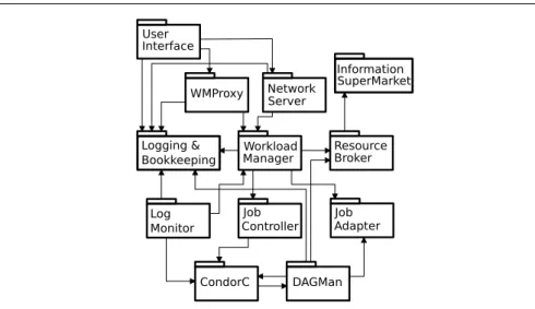
The EGEE WMS is seen from the user’s perspective as a two-levels batch system: the User Interface (client) connects to a Workload Manager System (WMS). The WMS is interfaced to the grid Information System to obtain indications on the grid sites status and workload conditions. It queues user requests and dispatches them to one of the sites connected. The sites receive grid jobs through a gateway known as Computing Element (CE). Jobs are then handled through the sites’ local batch systems. To comprehend the complexity of the system, a more complete view of the WMS architecture, extracted from the WMS user guide [18] is depicted in figure 1.
When submitting a job, the client User Interface connects to the core Workload Manager through a WMProxy Web Service interface or the Network Server. The Work-load Manager queries the Resource Broker and its Information SuperMarket (repository of resources information) to determine the target site that will handle the computation task, taking into account the job specific requirements. It then finalizes the job submis-sion through the Job Adapter and delegates the job processing to CondorC. The job
Fig. 1 gLite Workload Management System architecture; source: WMS user guide.
evolution is monitored by the Log Monitor (LM) which intercepts interesting events (affecting the job state machine) from the CondorC log file. Finally, the Logging and Bookkeeping service (LB) logs job events information and keeps a state machine view of the job life cycle. The user can later on query the LB to receive information on her job evolution.
For load balancing and system scalability, the EGEE infrastructure operates around a hundred of similar WMS. However, these WMSs largely share the same population of connected CEs and, as they are not interconnected, do not perform across WMSs load balancing. Instead, WMSs are indirectly updated of the overall workload condition variations through information collected by the information supermarket. It is up to the clients to select their WMS at submission time. The client User Interface implements a simple round-robin WMS selection policy to assist users in their job submission process. In the remainder we are particularly interested in the impact of the grid middleware on the job execution time, i.e. the latency induced by the middleware operation, that is not related to the job execution itself. This latency is a measure of the middleware overhead. In case of faults (scheduling problems, middleware faults...) this latency will arbitrarily increase and to prevent application blocking the job needs to be considered lost after a long enough waiting time.
2.2 Jobs’ life cycle
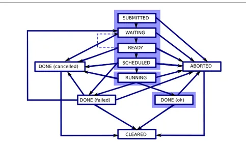
The jobs’ life cycle is internally controlled through a state machine displayed in figure 2 [18] where states and possible transitions are presented.
The normal states assigned to a job are underlined in boxes with thick borders (they correspond to the case of a job completed successfully):
SUBMITTED: the job was received by the WMS and the submission event is logged in the LB.
WAITING: the job was accepted by WM, waiting to match a CE. READY: the job is sent to its execution CE.
Fig. 2 Jobs life cycle state machine; source: WMS user guide.
SCHEDULED: the job is queued in the CE batch manager RUNNING: the job executes on a worker node of the target site DONE (ok): the job completed successfully.
CLEARED: after outputs of a completed job have been retrieved by the user, the job is cleared. In case of non completion of job, files are cleared by the system. Other states may also be encountered:
ABORT: in any state, the middleware can abort the operation. An additional status reason is usually returned.
DONE (failed): some errors may prevent correct job completion. An additional status reason is usually returned.
DONE (cancelled): the job was cancelled by the user.
2.3 Grid observatory
The basis of our work on the WMS behavior modeling is the collection of statistical information on job evolution on the live grid infrastructure. The relevant information for performance modeling is the duration of jobs, including fine details on the interme-diate times spent between transitions of the state diagram. This information collection step is difficult in itself and the means of collecting relevant data will depend on the targeted exploitation of the model. To deal with jobs resubmission on the client side, information needs to be collected actively by the client or through a dedicated ser-vice accessible from the client. Conversely, on the WMS server-side, quite extensive monitoring information on the jobs handled by this server is available and could be exploited.
In a previous work focussing on client-side submission strategies [14], we collected such information via periodic probe jobs submissions and life-cycle tracking on the infrastructure. Although this strategy is easy to implement (all that is needed is a user interface connected to the infrastructure), it is both restrictive (the polls are specific
short duration jobs, the jobs are limited to the resources accessible to the specific user performing submission) and has limited accuracy (only a limited number of polls can be simultaneously submitted to avoid disturbing normal operation, the traces are collected by periodic polling and the period selected impacts the accuracy of results). A more satisfying approach is to collect traces from regular jobs submitted on the grid infrastructure during normal grid operation, thus assembling a complete and accurate corpus of data. However, there are more difficulties in implementing this approach than would be expected, including:
– traces are recorded by different inter-dependent services (WM, CondorC, LM, LB...) that are tracing partly redundant and partly complementary information; – traces are collected on many different sites (operating different WMSs)
adminis-trated independently: agreement to collect the data has to be negotiated with the (many) different site administrators;
– different versions of the middleware services co-exist on the infrastructure and traces are produced by slightly varying sources (including changes in states, labels, spell fixing in messages returned, etc);
– traces are recorded on different computers which clocks are not always well syn-chronized (although NTP should be installed on every grid host);
– traces collected are incomplete as parts of them can be lost (log files loss, disk crashes, etc) and all job states are not always recorded (middleware latency and faults cause some transition losses);
– as it will appear in the rest of this paper, the traces recorded often do not match precisely the information documented in the existing guides (state name changes, etc).
The most accurate source of traces available on the EGEE grid today is the Real
Time Monitor6 (RTM) [4] implemented at the Imperial College London for the need
of real time grid activity monitoring and visualization. The RTM gathers information from EGEE sites hosting Logging and Bookkeeping (LB) services. Information is cached locally at a dedicated server at Imperial College London and made available for clients to use in near real time.
The system consists of three main components: the RTM server, the enquirer and an Apache Web server which is queried by clients. The RTM server queries the LB servers at fixed time intervals, collecting job related information and storing this in a local database. Job data stored in the RTM database is read by the enquirer every minute and converted to an XML format which is stored on the Web Server. This decouples the RTM server database from potentially many clients which could bottleneck the database.
The RTM also provides job summary files for every job as text files (“Raw Data”). These data are analysed off-line and fixed record length tuples are created on daily basis, one file per LB server. These files are used for the analysis presented in this paper.
An extended information about services offered by the RTM including detailed description of the system architecture can be found in [4].
The systematic collection of grid traces for studying grid systems has been rec-ognized as a key issue and significant effort has been recently invested in setting up the EGEE Grid Observatory which aims to collect information and ease access to it
REGISTERED RAN DONE 64.1 % REGISTERED ABORT 29.4 % REGISTERED DONE 2.7 % REGISTERED RAN ABORT 0.9 %
Table 1 Top 4 life cycle values with their frequencies
through a portal. The grid observatory has long term objectives of cleaning and har-monizing the data. It currently provides access to first body of data collected in Paris regional area (GRIF) and by the RTM.
3 Statistical data
The data considered in this study are RTM traces of the EGEE grid activity during the period from September 2005 to June 2007. 33,419,946 job entries were collected, each of them representing a complete job run. Among the information recorded in an entry can be found: the job ID, the resources used (UI, RB, CE, WN), the VO used, the job specific requirements, the job life cycle concatenated field and a complementary “final reason” text detailing the reason for the final state reached. Different epoch times are given, allowing the measurement of the duration of each step in the job life cycle: epoch regjob ui: registration of a job on a User Interface
epoch accepted ns: job accepted by the network server epoch matched wm: job matched to a target CE
epoch transfer jc: job accepted and being transferred to the CE epoch accepted lm: job accepted by the CE
epoch running lm: job started running (logged by the LM) epoch done lm: job completed (successfully or not)
epoch running lrms: job started running (logged by the LRMS) epoch done lrms: job completed (successfully or not)
The last two couples of epoch data can be redundant: one is given by the LM while the other is given by the local resource management system (LRMS) or batch system. The LM data is less accurate than the LRMS, but the LRMS data does not exist for all CEs.
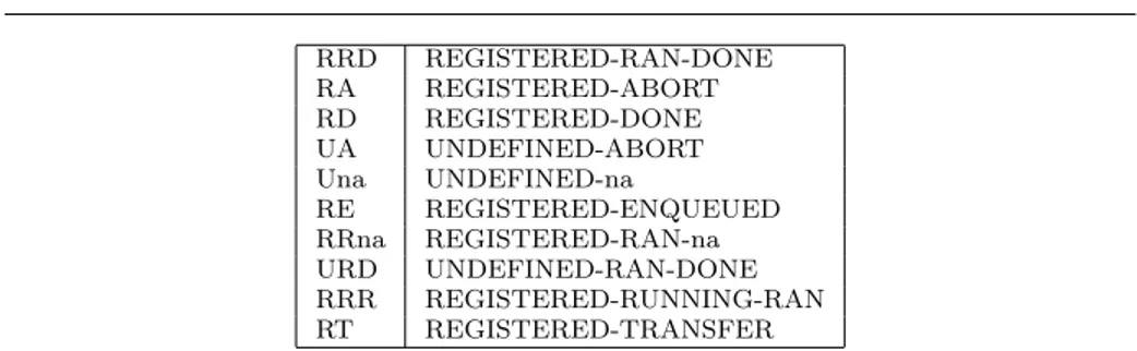
The life cycle field holds information on the different states the job has encoun-tered during its life cycle (see figure 2). It is composed of the concatenation of the different state names, considering some minor variations in names (e.g. RAN corre-sponds to a past RUNNING state; REGISTERED correcorre-sponds to a job registered on the UI it has been SUBMITTED to). In the data considered in this paper, 50 different values of the life cycle field have occurred with different frequencies. They corre-spond to different situations: job successfully terminated and data retrieved (REGIS-TERED RAN DONE CLEARED), job aborted (REGIS(REGIS-TERED ABORT), etc. The top 4 life cycle values with their frequencies are given in table 1. As all jobs encounter the “CLEARED” status, we have omitted this status in the remainder of the paper.
To give more information on the reason for the final state of a job (especially in case of error), the final reason field provides a user readable message. Unfortunately, the set of possible values is larger, due not only to the diversity of cases that may
RRD REGISTERED-RAN-DONE RA REGISTERED-ABORT RD REGISTERED-DONE UA UNDEFINED-ABORT Una UNDEFINED-na RE REGISTERED-ENQUEUED RRna REGISTERED-RAN-na URD UNDEFINED-RAN-DONE RRR REGISTERED-RUNNING-RAN RT REGISTERED-TRANSFER
Table 2 Abbreviations for some type values.
occur but also to the different versions of middlewares, sometimes displaying differ-ent messages for the same reason. Combined with the life cycle field, we counted 236 different cases. Some final reason fields were shortened to exclude non relevant specific information such as particular file name or site name appearing in the message. Before exploiting the data, some curation was needed for proper interpretation. Specifically: data sources were selected when redundant information was available (LM and LRMS traces redundancy); specific text final reason fields were truncated; and rare events were neglected in order to reduce the number of cases to analyze (an experimental justification is given in paragraph 5.3). As a result, table 3 details the 32 most frequent cases, representing 99.4% of the total data. This selection is a trade-off between data completeness and number of cases to analyze. The last column of table 3 proposes a classification of the cases into 3 classes that are detailed below.
3.1 Successful jobs
The first class corresponds to jobs that have started running and either terminated successfully or were canceled by the user. We consider that these jobs were possibly successful even if the intervention of the user changed the final status or if some pro-duced files were not retrieved or used. For these jobs, we denote by R the job latency, i.e. the time between the epoch of registration on the UI and the epoch where the job starts running. Due to some clock synchronization problems it may happen that a latency value R is negative: such entries have been excluded from the study. Such problems may also alter some positive values. However, these events are rare and the synchronisation difference are small compared to the values considered.
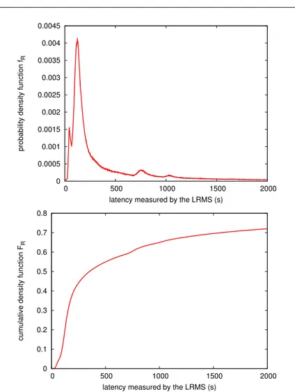
As LRMS values are more accurate, we decided to keep only data where LRMS values were available. The number of remaining traces is given for each case in table 3 inside the parenthesis after the R symbol. This class is composed of 18,991,905 entries. Figure 3 displays the distribution of latency values for all successful cases from table 3. We observe that all profiles are similar although the frequencies differ, and the first class represents most of the data. Figure 4 displays the probability density
function (fR) of the latency on top and its cumulative density function (FR) on bottom.
These laws are known to be heavy tailed [9] meaning that the tail is not exponentially bounded (see figure 5):
∀λ > 0, lim
t→∞e
λt
0 10000 20000 30000 40000 50000 60000 0 500 1000 1500 2000
occcurence of latency value
latency measured by the LRMS (s) 1 4 6 5 6 12 13 21 23 24 22 26 29 0 2000 4000 6000 8000 10000 12000 14000 16000 0 100 200 300 400 500
occcurence of latency value
latency measured by the LRMS (s) 1 4 6 5 6 12 13 21 23 24 22 26 29
Fig. 3 Occurrences of latency values for different cases (see table 3) of successful jobs. The figure below gives more details for low values. The first two cases (1 and 2) are plotted thicker for an easier reading.
case type and final reason occurrences % class
1 RRD Job terminated successfully 17,202,969 51.5% R (15,035,704) 2 RA Job RetryCount (0) hit 3,838,380 11.5% outlier 3 RA Cannot plan: BrokerHelper: no compa 3,422,319 10.2% F
4 RRD - 2,176,464 6.51% R (1,888,797) 5 RRD There were some warnings: some file 1916300 5.74% R (1,698,337) 6 RD Aborted by user 863,094 2.58% R (875,89) 7 RA Job RetryCount (3) hit 582,152 1.74% outlier
8 RA - 557,055 1.67% F
9 RA Job proxy is expired. 495,519 1.48% F 10 RA cannot retrieve previous matches fo 358,726 1.08% F 11 RRA Job proxy is expired. 267,890 0.80% F
12 Una - 235,458 0.70% R (10,632)
13 RRD Aborted by user 188,421 0.56% R (15,3479) 14 RA Job RetryCount (1) hit 165,231 0.49% outlier 15 UA Error during proxy renewal registra 149,095 0.45% F 16 RA Unable to receive 115,867 0.35% F
17 RE - 109,089 0.33% F
18 RA Cannot plan: BrokerHelper: Problems 89,553 0.27% F 19 UA Unable to receive 70,215 0.21% F 20 RA Job RetryCount (2) hit 63,595 0.19% outlier
21 RRna - 56,044 0.17% R (53,055)
22 RRD There were some warnings: some outp 49,046 0.15% R ( 38,656)
23 RD - 45,400 0.14% R (2,091)
24 URD Job terminated successfully 31,722 0.09% R (236)
25 RRA - 26,268 0.08% F
26 RRR - 22,983 0.07% R (19561)
27 RA Submission to condor failed. 22341 0.07% F 28 RA Job RetryCount (5) hit 22,260 0.07% outlier 29 RT Job successfully submitted to Globu 18,972 0.06% R (3,768) 30 RT unavailable 18,065 0.05% F 31 RA Job RetryCount (7) hit 17,328 0.05% outlier 32 RA hit job shallow retry count (0) 16,863 0.05% outlier
Table 3 The 32 most frequent cases of type and final reason field values are totalizing 99.4% of the total data. Type values have been abbreviated for readability, using short names from table 2. The last column distinguishes correctly running jobs with latency (R with number of data entries remaining after cleaning), failed jobs (F) and outliers.
3.2 Failed jobs
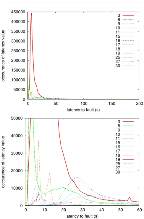
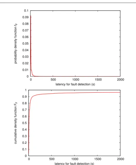
The second class corresponds to jobs that have failed for different reasons, leading to abortion by the WMS (no compatible resources, proxy error, BrokerHelper problem, CondorC submission failure...). Most jobs are aborted after a delay, denoted by the variable F , computed from the epoch of job registration until the done state epoch corresponding to the abortion instant. The delay F is one of the subjects of this study. Similarly to the previous class, some synchronization clock problems led to exclude some data. Moreover, the terminal “done” status may not be reached in some cases, as for example 15 and 19. We have decided to assume that the fault was immediately reported to the system in these cases. This class is finally composed of 5,607,329 entries. The different fault latency profiles (F ) for the different cases of table 3 labelled as faults are displayed in figure 6. Contrarily to the study of successful jobs, we observe that the profiles of the curves corresponding to each case conducting to fault are quite different. The corresponding probability density function (pdf) and cumulative density
0 0.0005 0.001 0.0015 0.002 0.0025 0.003 0.0035 0.004 0.0045 0 500 1000 1500 2000
probability density function f
R
latency measured by the LRMS (s)
0 0.1 0.2 0.3 0.4 0.5 0.6 0.7 0.8 0 500 1000 1500 2000
cumulative density function F
R
latency measured by the LRMS (s)
Fig. 4 Probability density function (top) and cumulative density function (bottom) of the latency in all the cases displayed in figure 3.
function (cdf) of F are plotted in figure 7. They correspond approximately to the profile of case number 3 even if they have been computed on all failed jobs: case number 3 is predominant (10.2% of entries compared to second larger, case number 11 with 1.67% of entries).
3.3 Outliers
Jobs with type “REGISTERED-ABORT” and final reason “Job RetryCount (any num-ber) hit” are jobs that have failed at least once at a site and been submitted to other sites until the user defined maximum number of retries is reached at which point the WMS gives up on the jobs. The WMS is aware of such failures either because it is notified of the job failure or because the job times out.
0 2000 4000 6000 8000 10000 0 2000 4000 6000 8000 10000 exp( λt)(1-F R (t)) t = latency (s) λ=1 λ=0.1 λ=0.01 λ=0.001
Fig. 5 Product eλt(1 − FR(t)) for different values of λ where FR is the cumulative density
function of the latency. This illustrates that the distribution of latency is heavy tailed.
The final reason for a large part of these jobs is known after a very long delay (few 100000s seconds) when compared to other failed jobs. They correspond to jobs that never return due to some middleware failure or network interruption (jobs may have been sent to a CE that has been disconnected or crashed and the LB will never receive notification of the completion). They are usually detected using a timeout value by the WMS. This last class of jobs, labelled as outliers, contains 4,705,809 entries.
3.4 Summary
We denote as ρ the ratio of outliers and φ the ratio of faulty jobs. In the complete data set considered, we measure the following ratios:
outliers : ρ = 16.1%
faults : φ = 19.1%
successful : 1 − ρ − φ = 64.8%
Even if the ratio of jobs that have started running is the highest (64.8 %), the ratios of outliers or failed jobs are high: they have to be taken into account when working on such production grid.
When comparing the distribution of F to the one of R, we observe that, even if faults are not always known immediately, they are usually identified in a shorter time than the latency impacting most successful jobs. We will now study the impact of the delay before faults detection on the total latency of a job, including resubmissions after faults.
0 50000 100000 150000 200000 250000 300000 350000 400000 450000 0 50 100 150 200
occcurence of latency value
latency to fault (s) 3 8 9 10 11 15 16 17 18 19 25 27 30 0 10000 20000 30000 40000 50000 0 10 20 30 40 50 60
occcurence of latency value
latency to fault (s) 3 8 9 10 11 15 16 17 18 19 25 27 30
Fig. 6 Occurrences of latency to fault values for different cases (see table 3) and detail for low values. The first two cases (3 and 8) are plotted thicker for an easier reading.
0 0.01 0.02 0.03 0.04 0.05 0.06 0.07 0.08 0.09 0.1 0 500 1000 1500 2000
probability density function f
F
latency for fault detection (s)
0 0.1 0.2 0.3 0.4 0.5 0.6 0.7 0.8 0.9 1 0 500 1000 1500 2000
cumulative density function F
F
latency for fault detection (s)
Fig. 7 pdf (top) and cdf (bottom) of the latency for fault detection in all the cases examined in figure 6.
4 Resubmission after fault 4.1 Probabilistic modeling
In the remainder, a capital letter X traditionally denotes a random variable with
probability function (pdf) fXand cumulative density function (cdf) FX. Let R denote
the latency of a successful job and F denote the failure detection time. Thus, FRand
fRdenote the cdf and pdf of the latency R while FF and fF denote the cdf and pdf
of failure detection time.
Assuming that faulty jobs are resubmitted without delay, let L denote the job latency taking into account the necessary resubmissions (without any limit on the number of resubmissions). L depends on the distribution of the jobs failure time. With
ρ the ratio of outliers and φ the ratio of failed jobs, the probability, for a job to succeed is (1 − ρ − φ).
A job encounters a latency L < t, t being fixed, if it is not an outlier and either: – the job does not fail (probability (1 − ρ − φ)) and its latency R < t (probability
P (R < t) = FR(t)); or
– the job fails at t0< t (probability φfF(t0)) and the job resubmitted encounters a
latency L < (t − t0)
The cumulative distribution of L is thus defined recursively by:
FL(t) = (1 − ρ − φ)FR(t) + φ
Z t
0
fF(t0).FL(t − t0)dt0
where the distributions of R and F are for instance numerically estimated from the statistical data set described in the previous section. However, in this equation, the cdf
FL appears both in left and right sides. Moreover, its value at time t does appear in
both terms.
In order to compute the cdf FL, we discretize this equation with some
considera-tions:
– No successful job has a null latency: FR(0) = 0
– We introduce the second as the discretization step for the variable t. Indeed, in practice we know that we cannot have a higher precision than the second for our measurements. The discretization step is chosen accordingly.
– Some jobs are immediately known to fail (for example if the fault occurs on the
client side). We thus consider FF(0) 6= 0
Since no job has a null latency, this is also the case with resubmitted jobs: FL(0) =
0. Supposing now t > 1, we get:
FL(t) = (1 − ρ − φ)FR(t) + φ
t−1
X
t0=0
fF(t0)FL(t − t0)
This equation is resolved differently in the cases t = 1 and t > 1. For t = 1, it simplifies to:
FL(1) = (1 − ρ − φ)FR(1) + φfF(0)FL(1) ⇒ FL(1) =
1 − ρ − φ
1 − φfF(0)
FR(1)
For t > 1, we can write:
FL(t) = (1 − ρ − φ)FR(t) + φfF(0)FL(t) + φ t−1 X t0=1 fF(t0)FL(t − t0) leading to: FL(t) = 1 1 − φfF(0) (1 − ρ − φ)FR(t) + φ t−1 X t0=1 fF(t0)FL(t − t0)
On the right side of this equation, the terms in FL are in the form FL(u) with u ∈
[1 ; (t − 1)]. FL(t) can therefore be computed recursively. The complete formula is
0 0.1 0.2 0.3 0.4 0.5 0.6 0.7 0.8 0.9 1 0 2000 4000 6000 8000 10000 12000 14000 16000 18000 20000
cumulative density functions
latency (s)
FL
(1-ρ)FR
FR
FF
Fig. 8 cdfs: latency of fault detection (FF), latency of successful jobs (FR), latency of
suc-cessful jobs using resubmission in case of failures (FL). For comparison: ˜FR= (1 − ρ)FR.
FL(0) = 0 FL(1) = 1 − ρ − φ 1 − φfF(0) FR(1) FL(t > 1) = 1 1 − φfF(0) " (1 − ρ − φ)FR(t) + φ t−1 X u=1 fF(t − u)FL(u) # (1)
4.2 Exploitation of the grid traces
Figure 8 displays the cdfs of several variables. FR and FF have been estimated from
the grid traces data. Equation 1 enables us to compute FL, the cdf of successful jobs
including resubmission in case of failures. We clearly observe the impact of failures in
this latency L when compared to R. FL’s curve is lower: the probability of achieving
a given latency when faults occur is thus lower. In order to see more precisely the
impact of failures, we also plotted (1 − ρ)FR which corresponds to the outliers and
the successful jobs, ignoring failed jobs. This last curve is slightly above FL: while L
displays a probability of 50% for jobs to have a latency lower than 761 seconds, it reduces to 719 seconds when ignoring failures (or the difference of probability is 1% for the same latency value).
Having established the distribution properties of L, we will now focus on the ex-ploitation of the data for implementing a realistic resubmission strategy that aims at reducing the latency experienced by users.
5 Resubmission strategy 5.1 Modeling
As seen in the previous section, the probability for a job to start execution before a
given instant t is given by FL(t). We consider the resubmission strategy developed in [9]
where a job is canceled and resubmitted if its latency R is higher than a given timeout
value t∞ which value needs to be optimized. The work presented in [9] was based on
probe jobs that neglected faults (they were excluded from the data) but some jobs did
not return and were labelled as outliers. We denote ˜FR(t) the probability for a job to
face a latency lower than t. When neglecting faults, ˜FR is related to the distribution
of latency FRand the ratio of outliers:
˜
FR(t) = (1 − ρ)FR(t)
We denote J the total latency including resubmissions after waiting periods of t∞.
From [9], we can express the expected total latency EJ, considering resubmissions at
t∞as: EJ(t∞) = 1 ˜ FR(t∞) Z t∞ 0 (1 − ˜FR(u))du (2)
Thanks to the more complete workload data studied in this paper, we can refine the model by taking the latency for fault detections into account. We thus consider the following resubmission strategy: jobs for which the latency L, including resubmissions
due to failures, is greater than a timeout value t∞ are canceled and resubmitted.
Observing that FL(t) corresponds to the probability for a job to succeed with a latency
lower than t, we can replace, in equation 2, ˜FRby FL:
EJ(t∞) = 1
FL(t∞)
Z t∞
0
(1 − FL(u))du (3)
Minimizing this equation leads to the estimation of the optimal timeout t∞ value.
5.2 Impact of taking into account faults in the model
The profile of the expectation of the total latency, including all resubmissions and computed from equation 3 is plotted in figure 9. The curve reaches a minimum value
EJ = 584s for an optimal timeout value t∞ = 195s. The first part of the curve is
decreasing fast since underestimating the timeout value leads to cancel jobs that could have started running shortly. The second part of the curve is increasing, corresponding of a too long timeout value: jobs could have been canceled earlier.
Two more profiles are plotted for comparison. The first one is the case ignoring
the failures and corresponding to equation 2 with ˜FR = (1 − ρ)FR. Ignoring failures
conducts to underestimate the total latency: we observe that this plot is under the
previous one in figure 9. In that case, the minimum is reached at t∞= 191s, leading
to EJ= 529s which is under-evaluated.
The second comparison is performed with the assumption that failures can be
considered as outliers, thus leading to a total of 35% of outliers. In this case, EJ
0 500 1000 1500 2000 0 100 200 300 400 500 600
expectation of total latency E
J
timeout value (s)
EJ (equation 3)
without fault with faults as outliers
Fig. 9 Expectation of total latency with respect to timeout value t∞. The first curve is
obtained from equation 3. The result is compared with the case ignoring failures and the case where failures are accounted as outliers.
value EJ = 704s, highly overestimated. This is explained by the fact that failures
detection time is quite short (few seconds) and that waiting for t∞ instead of failure
detection time is penalising.
This experiment shows that taking into account a model of latency for faults to be detection has an influence on the parameters for this particular resubmission strategy.
5.3 Number of cases to consider
In section 3, we have retained the 32 most frequent cases, displayed in table 3. Here, results obtained with different numbers of most frequent cases are compared, in order to measure the relevance of reducing the number of cases to be taken into account.
Figure 10 presents the variation of EJwith respect to the timeout value t∞for different
numbers of most frequent cases. The optimal values of t∞leading to minimal EJvalues
are given in table 4. We observe that reducing the number of cases from 32 to 25 does not impact the results of the resubmission strategy, showing that not taking care of all possible cases (236 cases) does not impact the final result, since we are considering the most frequent ones.
However, reducing the number to 17 or less cases impacts the final result. In table 4, results concerning the model including faults and the previous model without including faults are displayed. These results show that reducing the number of cases to less than 17 cases impacts with the same order of magnitude than not considering the faults in the model. Our strategy considering faults in the model does have sense only if we consider more than 17 cases.
500 550 600 650 700 750 800 100 150 200 250 300 350 400 450 500
expectation of total latency E
J timeout value (s) 32 cases 25 cases 17 cases 7 cases 3 cases
Fig. 10 Variations of the expected total latency (EJ) including resubmissions with respect to
the timeout value, for different number of cases from table 3. We observe no visual difference between 32 and 25 cases. For less cases, we observe variations of EJ.
nb. of with faults (FL) without faults ( ˜FR)
cases opt. t∞ min. EJ opt. t∞ min. EJ
32 195s 584s 191s 529s 25 194s 584s 191s 529s 17 195s 577s 191s 524s 7 192s 558s 189s 530s 3 199s 606s 197s 570s
Table 4 Influence of the number of most frequent cases taken into account in the model on the estimation of optimal timeout value (t∞) and minimal expectation of total latency including
resubmission (EJ). Comparison of the results in two cases: with or without faults included in
the model.
5.4 Dynamic modeling and impact of grid workload conditions variation
Grid workload and faults occurrence are subject to significant variations through time. To assess the model validity over time, and its usability in a live use on a production infrastructure, we are considering the implementation of the model using probability density functions, outliers and failure rates estimated over shorter periods (typically one month). We also consider the error made when using the statistics of the month before to optimize jobs resubmission during the current month.
The 32 most frequent cases shown in table 3 have been analysed monthly over all the period of traces collection (September 2005 to June 2007). They represent from 89% to 98.6% of the data depending on the month considered, with a mean of 96%, confirming the hypothesis that it is possible to consider only these cases. Figure 11 presents the occurrences of each case for the different months of the study.
Distributions of latency for normal jobs execution and latency for fault detection have been computed for each month. Best timeout values and minimal expectation of total latency are thus computed on a monthly basis. Table 5 shows the corresponding results.
0 100 200 300 400 500 600 700 800 900 0 5 10 15 20 25 30 35
occurences of the case
case 2005-09 2005-10 2005-11 2005-12 2006-01 2006-02 2006-03 2006-04 2006-05 2006-06 2006-07 2006-08 2006-09 2006-10 2006-11 2006-12 2007-01 2007-02 2007-03 2007-04 2007-05 2007-06
Fig. 11 Occurrences of the first 32 cases of table 3, month by month. This shows that first cases are always the most frequent but not necessary in the same order as when considering all the data.
The second and third columns of table 5 show, for each month, the best timeout
value (t∞L) leading to the minimal expectation of total latency (EJL) with our model
considering faults (FL). They vary significantly according to different load conditions
and errors: the optimal timeout varies from 153s to 237s. It is important to take into account dynamic grid workload variations to optimize resubmission.
A practical use of the model introduced in this paper would require to estimate the statistical parameters of the model over a period and use these estimates over the next period. To study the performance of such a strategy, we have considered that we compute the timeout value at the end of each month and use it for the next month. The fourth column of table 5 shows the values of the expectation of total execution time using the optimal timeout value from the previous month, while considering faults
(EJL). Relative differences with the optimal EJL values computed a posteriori are
reported in the fifth column. The estimates present a mean error of 0.4%.
Impact of the data splitting into monthly time periods is studied using the sixth
and seventh columns where EJL is computed using the best timeout computed on
the whole set of data (see paragraph 5.2). The mean difference is only slightly higher (1.1%), showing that splitting the data into shorter time periods leads to a very small increase in the performance (at a cost that is also very small). However, it also shows that the impact of the time when the parameters of the strategy where computed is small. This is important since parameters are necessarily computed prior to their use.
6 Conclusions and perspectives
Probabilistic modeling of the grid jobs latency makes it possible to capture the complex behavior of grid workload management systems. The model proposed in this paper relies on statistics collection of job execution traces in order to estimate the cumulative density function of several parameters stochastically modeled. Compared to previous
prev. month whole set FL t∞L t∞L= 195s month t∞L EJL EJL ∆% EJL ∆% 2005-09 153 223 2005-10 159 282 283 0.3 292 3.6 2005-11 175 347 352 1.3 350 0.8 2005-12 181 293 293 0.1 294 0.5 2006-01 179 389 389 0.0 392 0.7 2006-02 171 530 531 0.3 541 2.1 2006-03 169 689 690 0.0 706 2.4 2006-04 183 453 457 0.9 454 0.3 2006-05 170 525 527 0.3 533 1.5 2006-06 170 599 599 0.0 609 1.7 2006-07 194 520 528 1.5 520 0.0 2006-08 186 699 701 0.3 701 0.3 2006-09 181 622 622 0.1 624 0.4 2006-10 198 724 730 0.9 724 0.0 2006-11 200 907 907 0.0 908 0.1 2006-12 197 719 719 0.0 719 0.0 2007-01 200 697 697 0.1 698 0.1 2007-02 237 899 916 1.9 923 2.6 2007-03 218 550 554 0.7 559 1.7 2007-04 209 544 544 0.2 547 0.6 2007-05 219 640 641 0.2 650 1.7 2007-06 234 758 760 0.2 780 2.8 mean 0.4 1.1
Table 5 In this table, the data set has been split monthly. For each month, best timeout (t∞L) and minimal expectation of total latency (EJL) have been computed using the model
including faults (FL). Then, a practical study has been done: the EJ value was computed
each month using the timeout computed the previous month or using the timeout computed from the whole set of data (t∞L = 195s). The last line displays the mean relative error of
the computed EJ with respect to the optimal EJL. Updating regularly the parameter of the
model gives the best results.
works, the model has been enriched to take into account normal operations, outliers and faults, which frequency is high on production grids and therefore significantly impacts job execution time. The model is exploited to optimize a simple job resubmission strategy that aims at optimizing applications performance using objective information. The more jobs a grid application is composed with, the more it will be sensitive to such fault recovery procedures.
This paper also emphasizes the practical difficulties encountered when collecting and then exploiting traces on a large scale, heterogeneous production grid infrastruc-ture. The set up of a Grid Observatory with well established procedures for traces collection, harmonization and curation is critical for the success of such grid behav-ioral analysis. It will allow to focus on modeling and experimentation without having to consider heavy-weight technical problems in the context of each new study. In addition, the Grid Observatory ensures dense data collection for accurate estimations without disturbing the normal grid operation.
The work detailed here exploits a consistent, archived set of traces for a posteriori analysis. It confirms that a production grid is prone to errors (faults and outliers). Measurements show that latencies of faults detection are usually smaller than latencies of running jobs. This observation was taken into account in the resubmission strategy modeled in the paper, including failed jobs. The classification of the jobs into successful,
failed and outliers has been done on a reduced set of type and final reason fields which has proved to be precise enough, and stable along time. We have simulated a practical
use of these results by computing the model parameter (t∞) on the data of a time period
for exploiting it during the following time period. This has shown that updating this model parameter reduces only slightly the total latency. This observation correlates with other ones [14].
In practice, a job resubmission strategy could be implemented at two different levels in the EGEE middleware: on the WMS server side to optimize the time-out value that is currently in use within the system, and also on the client side to deal with errors that are not handled and returned to the client. The server side implementation requires modifications to the existing middleware. It could benefit from the monitoring informa-tion collected by the WMS during normal operainforma-tions to provide needed statistics. The client side implementation can be wrapped above the existing client. Regardless of the server side strategy, it is important as a client may be disconnected from a WMS server to which it sent jobs due to network interruption of services or WMS overload, and it needs to take decisions on the resubmission strategy to adopt in that case. The client side implementation also requires statistics collection, that could be obtained from the regular jobs monitored and monitored by the client. The accuracy of the measurements then completely depends on the number of jobs managed. Alternatively, an external service collecting and exposing grid activity statistics in real-time could be envisaged. In the future, the Grid Observatory is expected to provide live information for tackling the non-stationarity of the grid workload manager and enabling relevant esti-mate of the grid running conditions. More elaborate submission strategies commonly implemented on grids, such as multiple submissions of a same task, will be considered. Such strategies are modeled in [15] but using a simplified model that does not take faults into account, which is an important parameter as illustrated in section 5.2.
Acknowledgements The datasets used in this work have been provided by the Grid Obser-vatory and the Imperial College London RTM. The Grid ObserObser-vatory is part of the EGEE-III EU project INFSO-RI-222667.
The authors warmly thank C´ecile Germain-Renaud (LAL-LRI Orsay) for founding the Grid Observatory, Stephen McGough (Imperial College London) who participated in this work-ing group and Gidon Moont, a previous RTM developer.
This work is partly funded by French National Agency for Research, NeuroLOG project, under contract number ANR-06-TLOG-024.
References
1. Aparicio, G., I. Blanquer Espert, and V. Hern´andez Garc´ıa: 2008, ‘A Highly Optimized Grid Deployment: the Metagenomic Analysis Example’. In: Global Healthgrid: e-Science Meets Biomedical INformatics (Healthgrid’08). pp. 105 –115.
2. Casanova, H., A. Legrand, and M. Quinson: 2008, ‘SimGrid: a Generic Framework for Large-Scale Distributed Experiments’. In: 10th IEEE International Conference on Com-puter Modeling and Simulation (UKSim). pp. 126–131.
3. Christodoulopoulos, K., V. Gkamas, and E. A. Varvarigos: 2008, ‘Statistical Analysis and Modeling of Jobs in a Grid Environment’. Journal of Grid Computing (JGC) 6(1), 77–101. 4. Colling, D., J. Martyniak, S. McGough, A. Kˇrenek, J. Sitera, M. Mulaˇc, and F. Dvoˇr´ak: 2009, ‘Real Time Monitor of Grid job executions’. In: Computing in High Energy Physics / Journal of Physics: Conference Series (CHEP 2009).
5. Dabrowski, C.: 2009, ‘Reliability in grid computing systems’. Concurrency and Computa-tion: Practice & Experience (CCPE) Special issue on Open Grid Forum 21(8), 927–959.
6. Feitelson, D.: 2002, Workload modeling for performance evaluation, pp. 114–141. Springer-Verlag - LNCS vol 2459.
7. Frachtenberg, E. and U. Schwiegelshohn: 2008, ‘New Challenges of Parallel Job Schedul-ing’. In: 13th Job Scheduling Strategies for Parallel Processing (JSSPP), Vol. LNCS 4942. pp. 1–23.
8. Germain, C., C. Loomis, J. T. Mo´scicki, and R. Texier: 2008, ‘Scheduling for Responsive Grids’. Journal of Grid Computing (JGC) 6(1), 15–27.
9. Glatard, T., J. Montagnat, and X. Pennec: 2007, ‘Optimizing jobs timeouts on clusters and production grids’. In: International Symposium on Cluster Computing and the Grid (CCGrid’07). pp. 100–107.
10. Huedo, E., R. S. Montero, and I. M. Llorente: 2006, ‘Evaluating the reliability of compu-tational grids from the end user’s point of view’. Journal of Systems Architecture 52(12), 727–736.
11. Hwang, S. and C. Kesselman: 2003, ‘A Flexible Framework for Fault Tolerance in the Grid’. Journal of Grid Computing (JGC) 1(3), 251–272.
12. Iosup, A., H. Li, M. Jan, S. Anoep, C. Dumitrescu, L. Wolters, and D. Epema: 2008, ‘The Grid Workloads Archive’. Future Generation Computer Systems (FGCS) 24(7), 672–686. 13. Li, H., D. Groep, and L. Walters: 2004, ‘Workload Characteristics of a Multi-cluster
Su-percomputer’. In: Job Scheduling Strategies for Parallel Processing. pp. 176–193. 14. Lingrand, D., T. Glatard, and J. Montagnat: 2009a, ‘Modeling the latency on production
grids with respect to the execution context’. Parallel Computing (PARCO) 35(10-11), 493–511.
15. Lingrand, D., J. Montagnat, and T. Glatard: 2009b, ‘Modeling user submission strate-gies on production grids’. In: International Symposium on High Performance Distributed Computing(HPDC’09). pp. 121–130.
16. Medernach, E.: 2005, ‘Workload Analysis of a Cluster in a Grid Environment’. In: Job Scheduling Strategies for Parallel Processing (JSSPP). pp. 36–61.
17. Nurmi, D., A. Mandal, J. Brevik, C. Koelbel, R. Wolski, and K. Kennedy: 2006, ‘Evaluation of a Workflow Scheduler Using Integrated Performance Modelling and Batch Queue Wait Time Prediction’. In: Conference on High Performance Networking and Computing. 18. Pacini, F.: 2006, ‘WMS User’s Guide’. Technical Report EGEE-JRA1-TEC-572489,
EGEE.
19. Swany, M. and R. Wolski: 2004, ‘Building Performance Topologies for Computational Grids’. International Journal of High Performance Computing Applications (IJHPCA) 18(2), 255–265.
20. Thebe, O., D. P. Bunde, and V. J. Leung: 2009, ‘Scheduling Restartable Jobs with Short Test Runs’. In: 14th Workshop on Job Scheduling Strategies for Parallel Processing (JSSPP’09), workshop: IPDPS, Vol. LNCS 5798. pp. 116–137.